CHAPTER 3
SUPERVISED LEARNING
NETWORK
“Principles of Soft Computing, 2nd
Edition”
by S.N. Sivanandam & SN Deepa
Copyright  2011 Wiley India Pvt. Ltd. All rights reserved.
DEFINITION OF SUPERVISED LEARNING NETWORKS
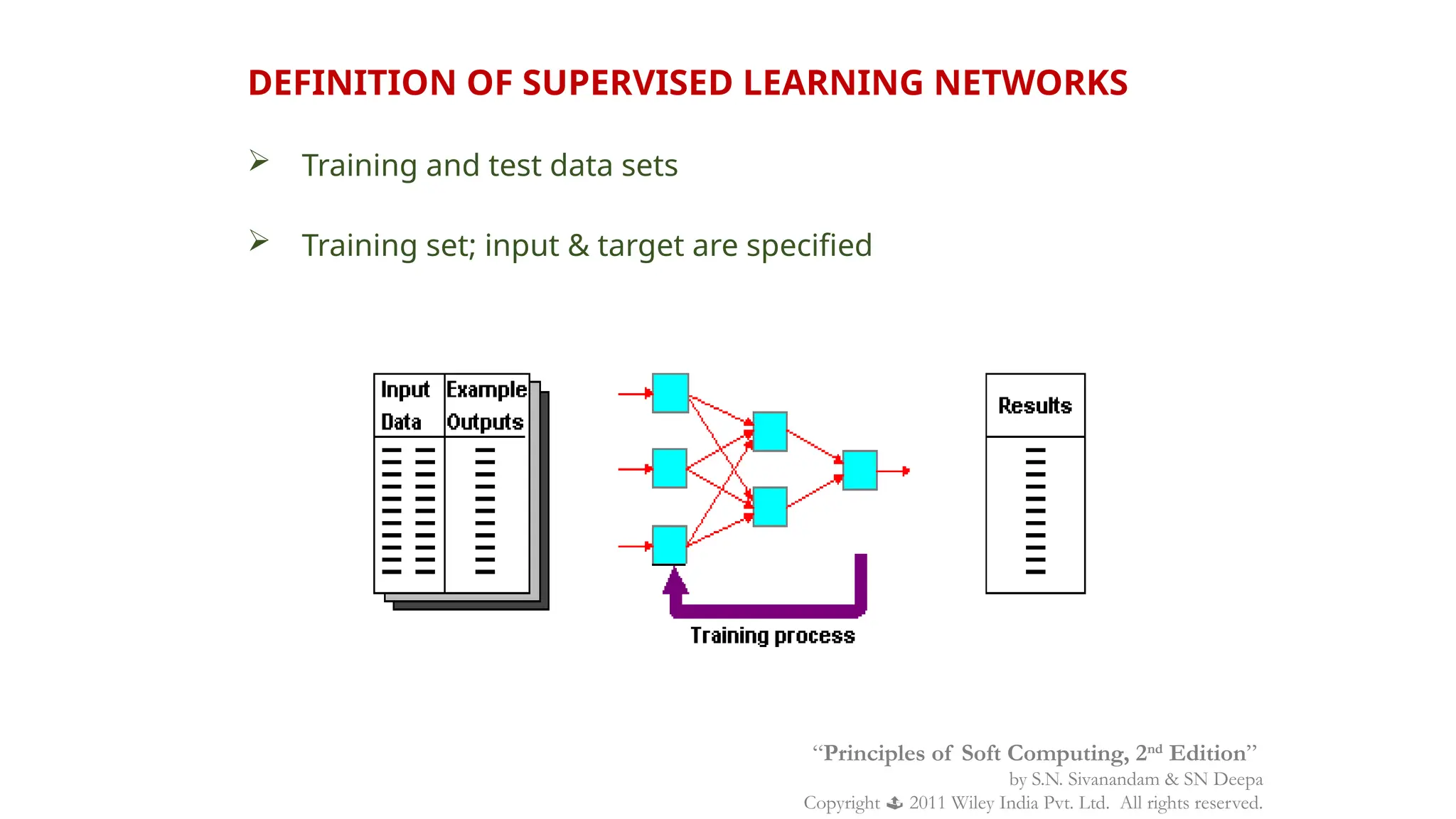
 Training and test data sets
 Training set; input & target are specified
“Principles of Soft Computing, 2nd
Edition”
by S.N. Sivanandam & SN Deepa
Copyright  2011 Wiley India Pvt. Ltd. All rights reserved.
PERCEPTRON NETWORKS
“Principles of Soft Computing, 2nd
Edition”
by S.N. Sivanandam & SN Deepa
Copyright  2011 Wiley India Pvt. Ltd. All rights reserved.
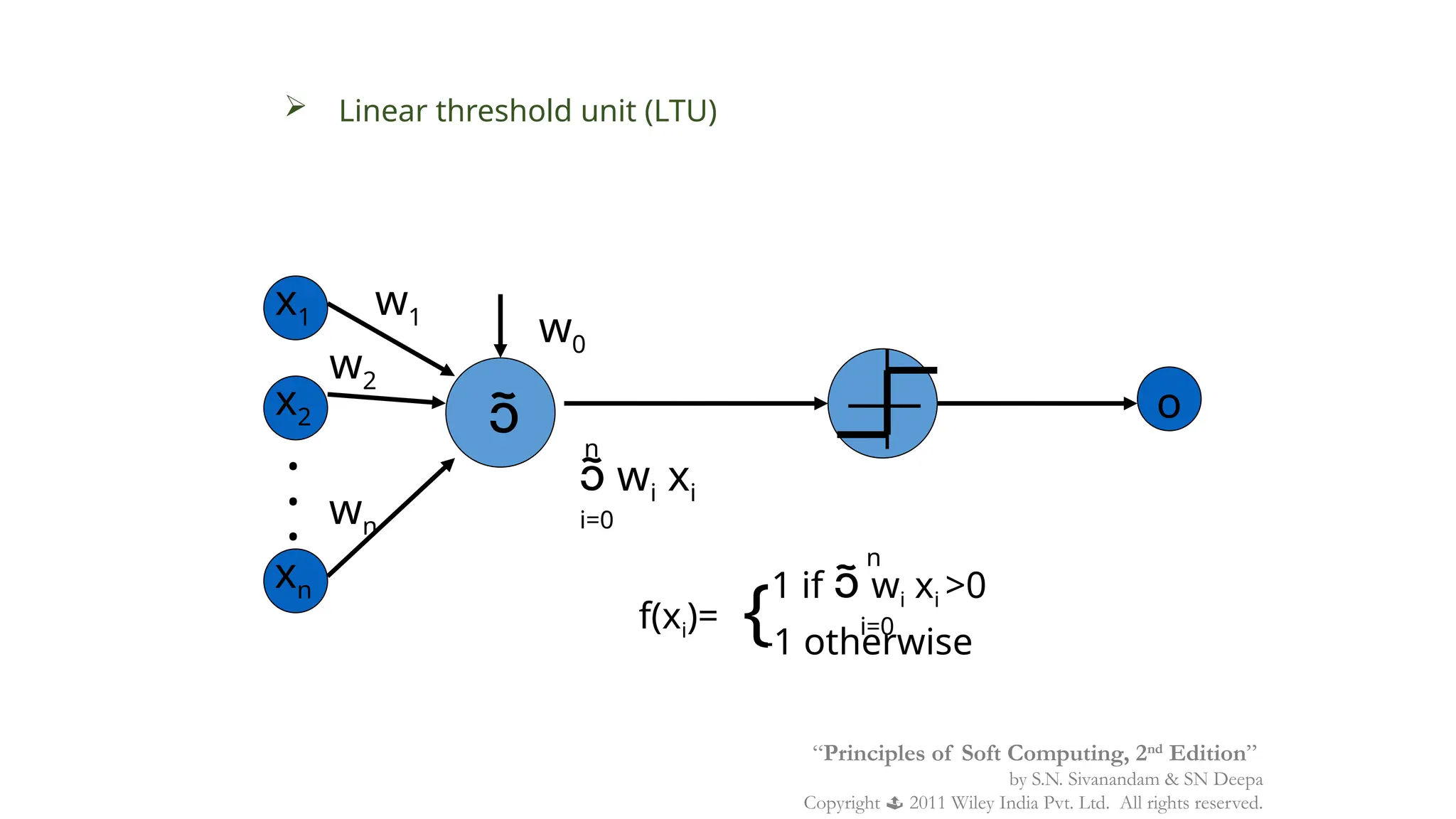
 Linear threshold unit (LTU)

x1
x2
xn
.
.
.
w1
w2
wn
w0
 wi xi
1 if  wi xi >0
f(xi)=
-1 otherwise
o
{
n
i=0
i=0
n
“Principles of Soft Computing, 2nd
Edition”
by S.N. Sivanandam & SN Deepa
Copyright  2011 Wiley India Pvt. Ltd. All rights reserved.
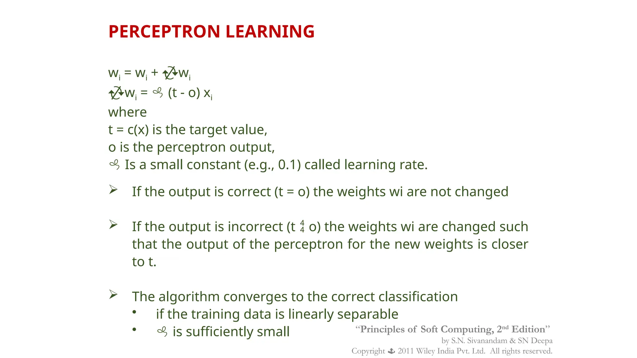
PERCEPTRON LEARNING
wi = wi + wi
wi =  (t - o) xi
where
t = c(x) is the target value,
o is the perceptron output,
 Is a small constant (e.g., 0.1) called learning rate.
 If the output is correct (t = o) the weights wi are not changed
 If the output is incorrect (t  o) the weights wi are changed such
that the output of the perceptron for the new weights is closer
to t.
 The algorithm converges to the correct classification
• if the training data is linearly separable
•  is sufficiently small “Principles of Soft Computing, 2nd
Edition”
by S.N. Sivanandam & SN Deepa
Copyright  2011 Wiley India Pvt. Ltd. All rights reserved.
LEARNING ALGORITHM
 Epoch : Presentation of the entire training set to the neural
network.
 In the case of the AND function, an epoch consists of four sets
of inputs being presented to the network (i.e. [0,0], [0,1], [1,0],
[1,1]).
 Error: The error value is the amount by which the value output
by the network differs from the target value. For example, if we
required the network to output 0 and it outputs 1, then Error =
-1.
“Principles of Soft Computing, 2nd
Edition”
by S.N. Sivanandam & SN Deepa
Copyright  2011 Wiley India Pvt. Ltd. All rights reserved.
 Target Value, T : When we are training a network we not only
present it with the input but also with a value that we require
the network to produce. For example, if we present the
network with [1,1] for the AND function, the training value will
be 1.
 Output , O : The output value from the neuron.
 Ij : Inputs being presented to the neuron.
 Wj : Weight from input neuron (Ij) to the output neuron.
 LR : The learning rate. This dictates how quickly the network
converges. It is set by a matter of experimentation. It is
typically 0.1.
“Principles of Soft Computing, 2nd
Edition”
by S.N. Sivanandam & SN Deepa
Copyright  2011 Wiley India Pvt. Ltd. All rights reserved.
TRAINING ALGORITHM
 Adjust neural network weights to map inputs to outputs.
 Use a set of sample patterns where the desired output (given
the inputs presented) is known.
 The purpose is to learn to
• Recognize features which are common to good and bad
exemplars
“Principles of Soft Computing, 2nd
Edition”
by S.N. Sivanandam & SN Deepa
Copyright  2011 Wiley India Pvt. Ltd. All rights reserved.
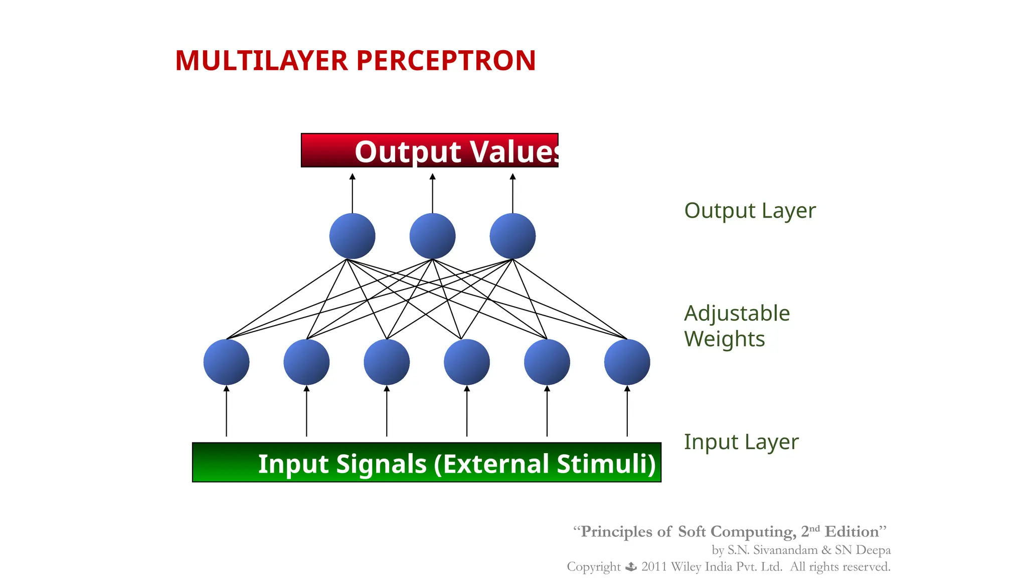
MULTILAYER PERCEPTRON
Output Values
Input Signals (External Stimuli)
Output Layer
Adjustable
Weights
Input Layer
“Principles of Soft Computing, 2nd
Edition”
by S.N. Sivanandam & SN Deepa
Copyright  2011 Wiley India Pvt. Ltd. All rights reserved.
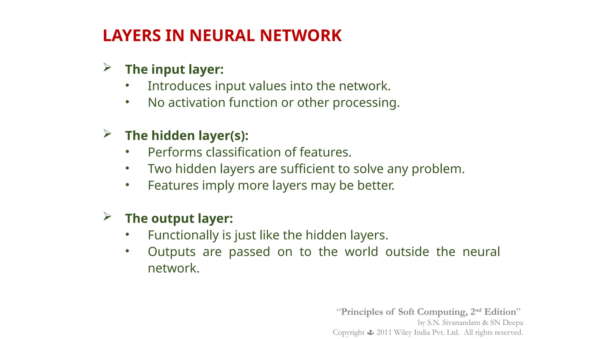
LAYERS IN NEURAL NETWORK
 The input layer:
• Introduces input values into the network.
• No activation function or other processing.
 The hidden layer(s):
• Performs classification of features.
• Two hidden layers are sufficient to solve any problem.
• Features imply more layers may be better.
 The output layer:
• Functionally is just like the hidden layers.
• Outputs are passed on to the world outside the neural
network.
“Principles of Soft Computing, 2nd
Edition”
by S.N. Sivanandam & SN Deepa
Copyright  2011 Wiley India Pvt. Ltd. All rights reserved.
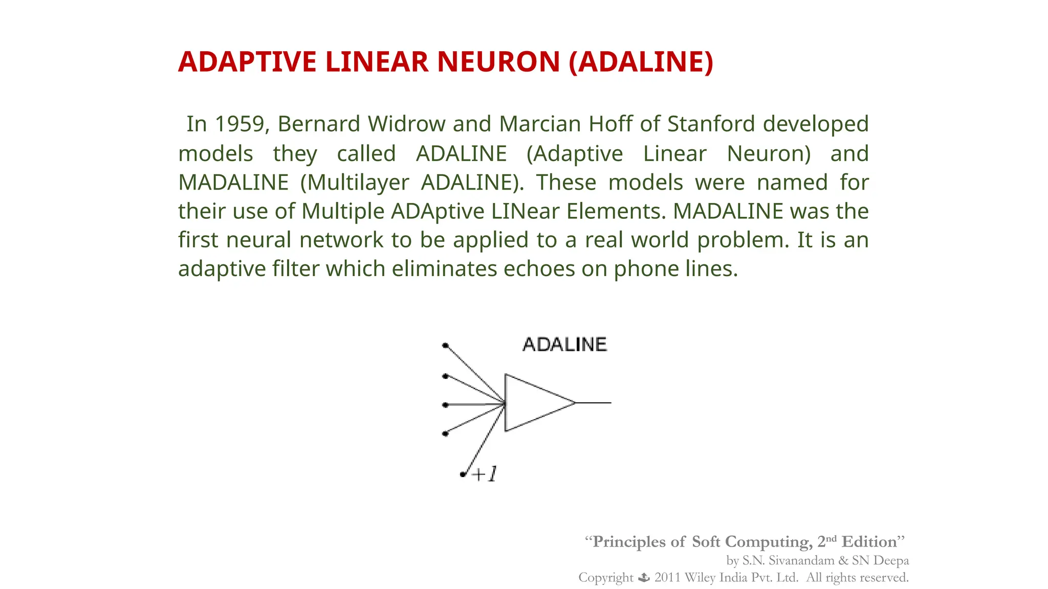
ADAPTIVE LINEAR NEURON (ADALINE)
In 1959, Bernard Widrow and Marcian Hoff of Stanford developed
models they called ADALINE (Adaptive Linear Neuron) and
MADALINE (Multilayer ADALINE). These models were named for
their use of Multiple ADAptive LINear Elements. MADALINE was the
first neural network to be applied to a real world problem. It is an
adaptive filter which eliminates echoes on phone lines.
“Principles of Soft Computing, 2nd
Edition”
by S.N. Sivanandam & SN Deepa
Copyright  2011 Wiley India Pvt. Ltd. All rights reserved.
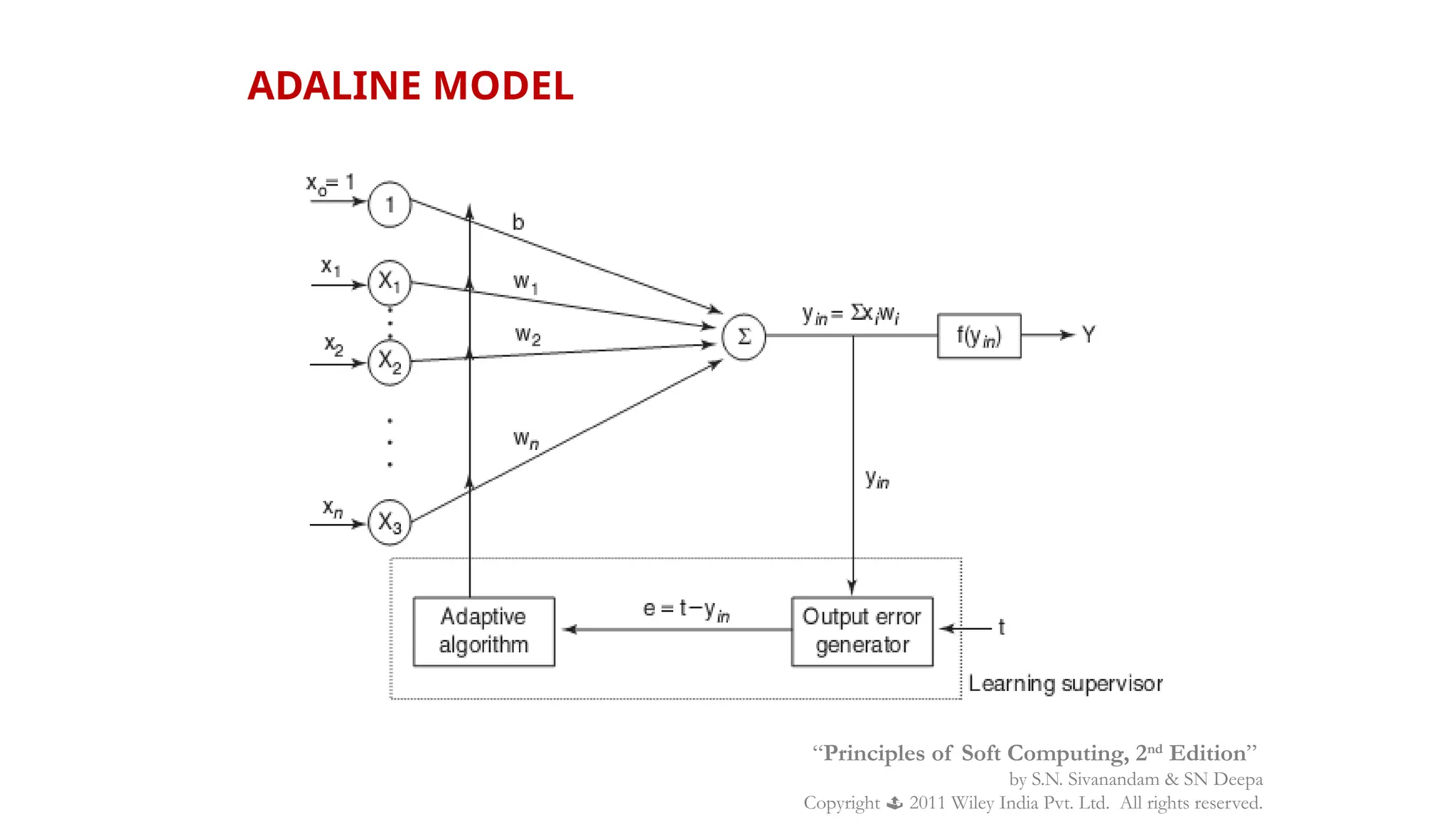
ADALINE MODEL
“Principles of Soft Computing, 2nd
Edition”
by S.N. Sivanandam & SN Deepa
Copyright  2011 Wiley India Pvt. Ltd. All rights reserved.
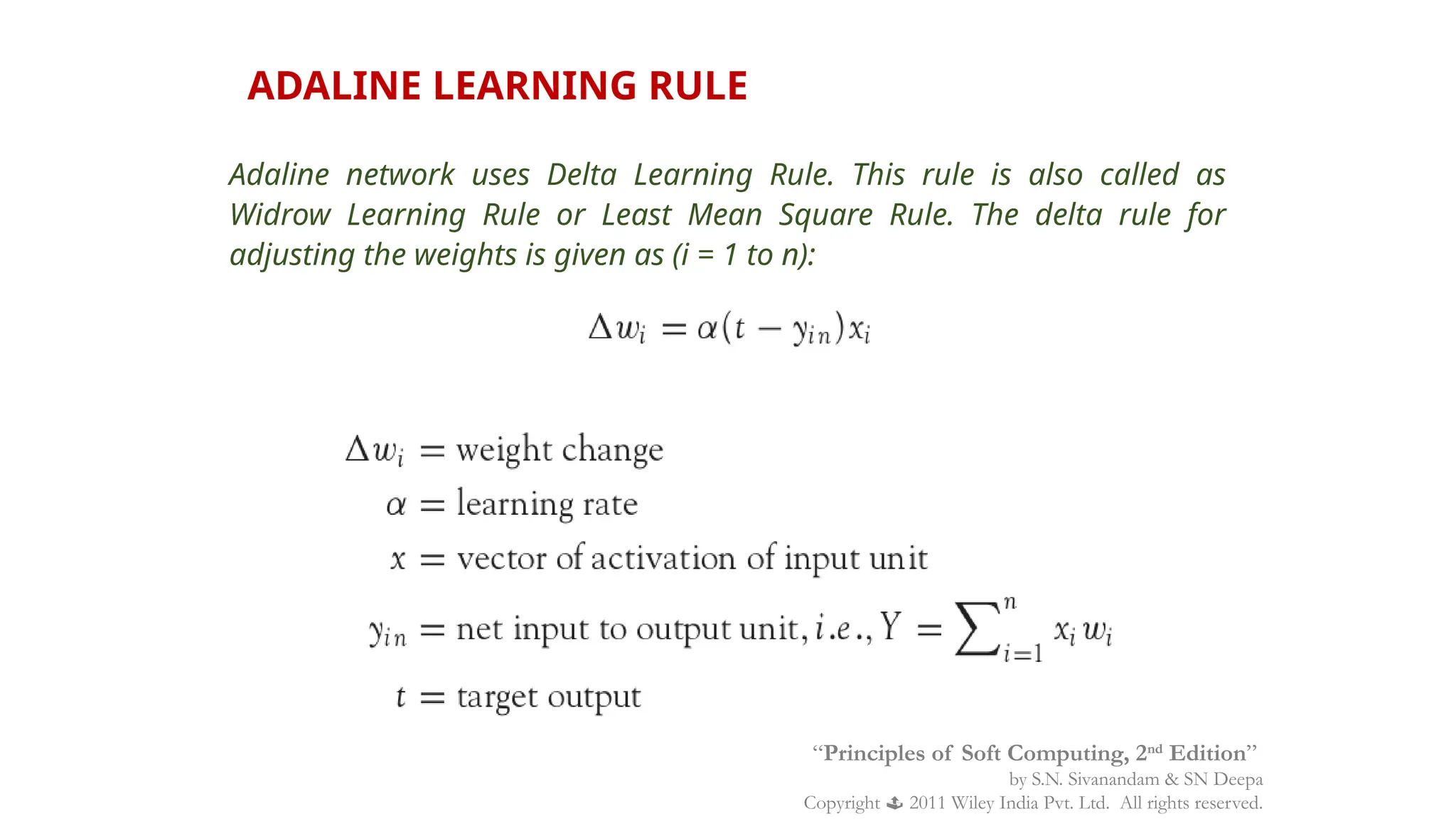
ADALINE LEARNING RULE
Adaline network uses Delta Learning Rule. This rule is also called as
Widrow Learning Rule or Least Mean Square Rule. The delta rule for
adjusting the weights is given as (i = 1 to n):
“Principles of Soft Computing, 2nd
Edition”
by S.N. Sivanandam & SN Deepa
Copyright  2011 Wiley India Pvt. Ltd. All rights reserved.
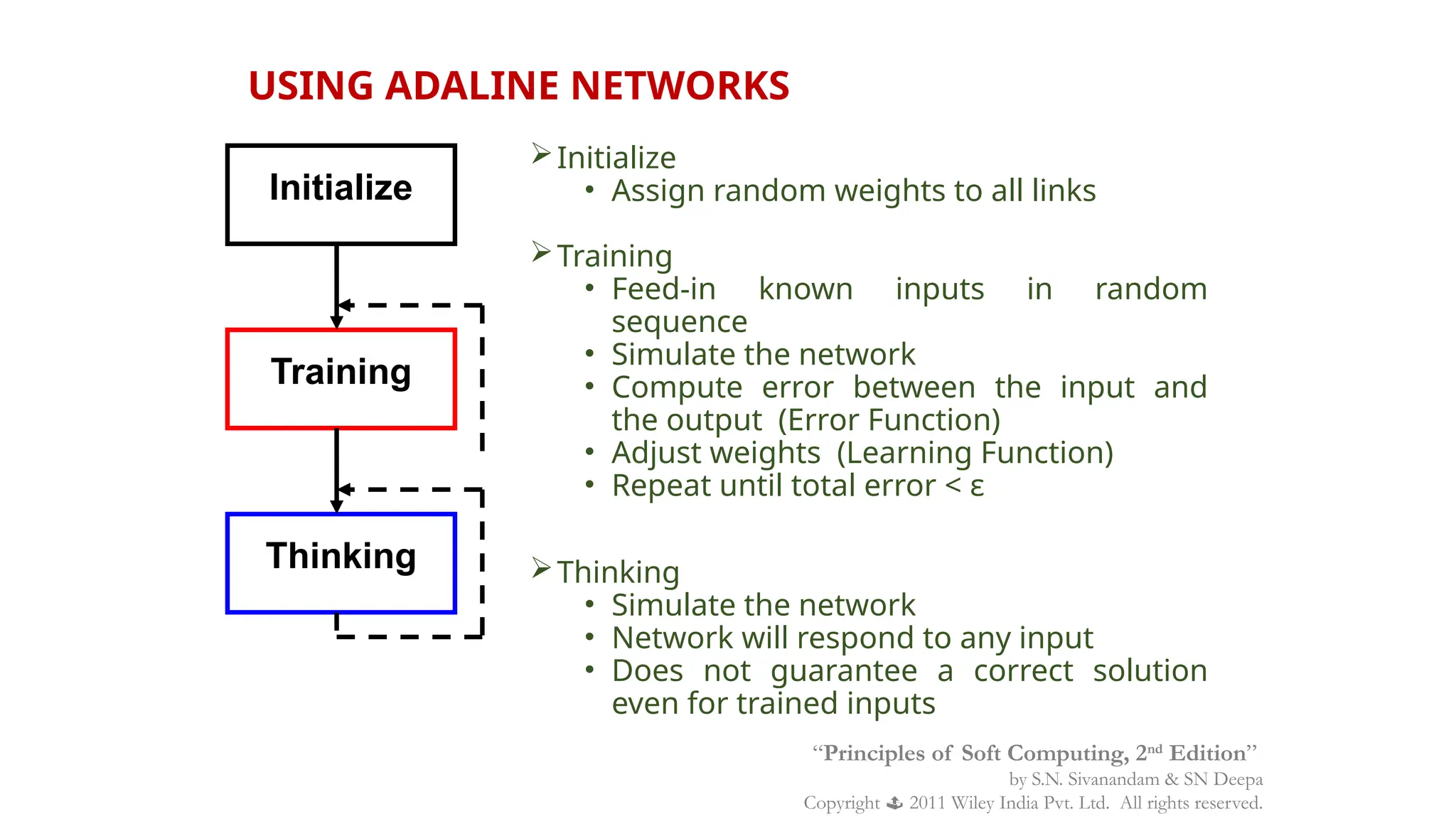
Initialize
• Assign random weights to all links
Training
• Feed-in known inputs in random
sequence
• Simulate the network
• Compute error between the input and
the output (Error Function)
• Adjust weights (Learning Function)
• Repeat until total error < ε
Thinking
• Simulate the network
• Network will respond to any input
• Does not guarantee a correct solution
even for trained inputs
USING ADALINE NETWORKS
Initialize
Training
Thinking
“Principles of Soft Computing, 2nd
Edition”
by S.N. Sivanandam & SN Deepa
Copyright  2011 Wiley India Pvt. Ltd. All rights reserved.
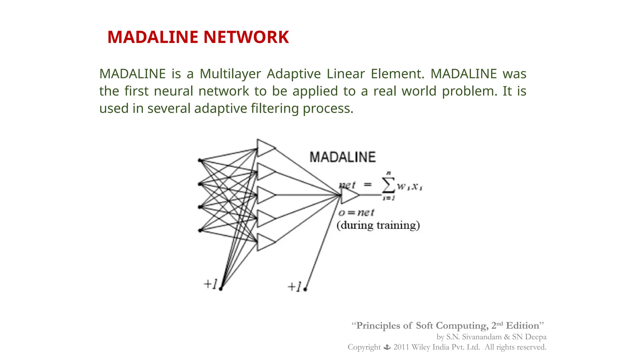
MADALINE NETWORK
MADALINE is a Multilayer Adaptive Linear Element. MADALINE was
the first neural network to be applied to a real world problem. It is
used in several adaptive filtering process.
“Principles of Soft Computing, 2nd
Edition”
by S.N. Sivanandam & SN Deepa
Copyright  2011 Wiley India Pvt. Ltd. All rights reserved.
BACK PROPAGATION NETWORK
“Principles of Soft Computing, 2nd
Edition”
by S.N. Sivanandam & SN Deepa
Copyright  2011 Wiley India Pvt. Ltd. All rights reserved.
 A training procedure which allows multilayer feed forward
Neural Networks to be trained.
 Can theoretically perform “any” input-output mapping.
 Can learn to solve linearly inseparable problems.
“Principles of Soft Computing, 2nd
Edition”
by S.N. Sivanandam & SN Deepa
Copyright  2011 Wiley India Pvt. Ltd. All rights reserved.
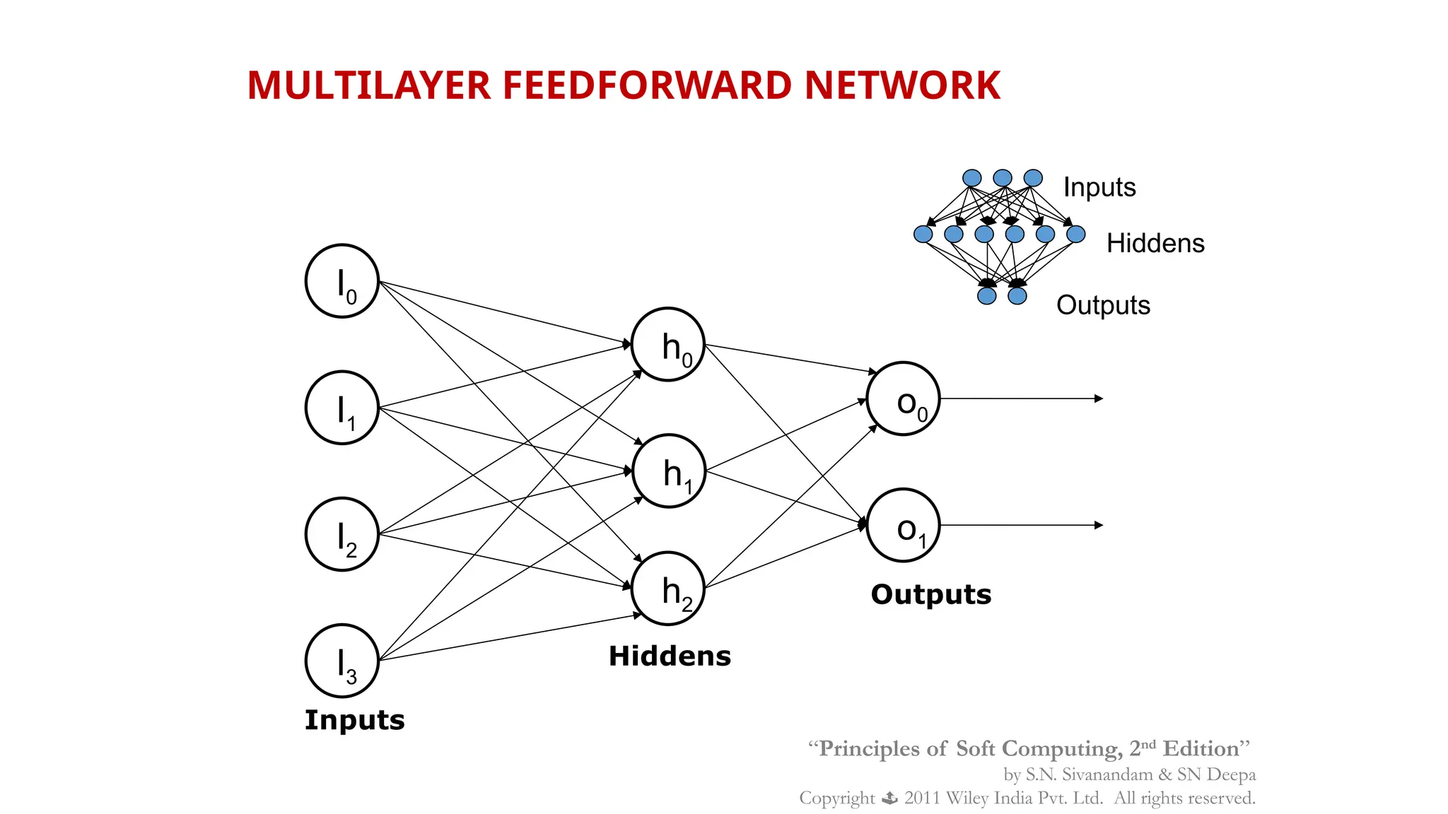
MULTILAYER FEEDFORWARD NETWORK
Inputs
Hiddens
Outputs
I1
I2
I3
I0
h0
h1
h2
o0
o1
Inputs
Hiddens
Outputs
“Principles of Soft Computing, 2nd
Edition”
by S.N. Sivanandam & SN Deepa
Copyright  2011 Wiley India Pvt. Ltd. All rights reserved.
MULTILAYER FEEDFORWARD NETWORK:
ACTIVATION AND TRAINING
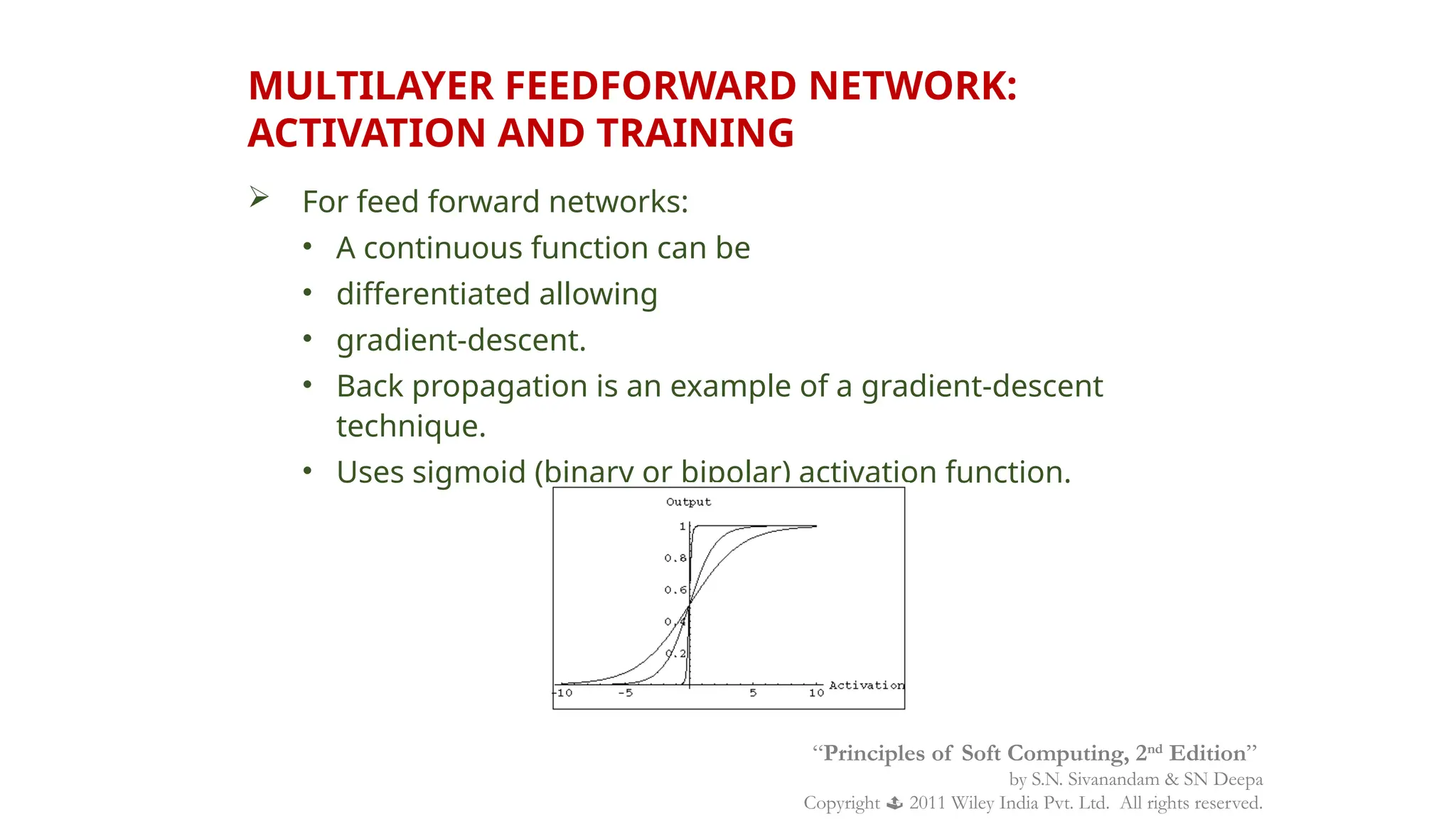
 For feed forward networks:
• A continuous function can be
• differentiated allowing
• gradient-descent.
• Back propagation is an example of a gradient-descent
technique.
• Uses sigmoid (binary or bipolar) activation function.
“Principles of Soft Computing, 2nd
Edition”
by S.N. Sivanandam & SN Deepa
Copyright  2011 Wiley India Pvt. Ltd. All rights reserved.
In multilayer networks, the activation function is
usually more complex than just a threshold function,
like 1/[1+exp(-x)] or even 2/[1+exp(-x)] – 1 to allow for
inhibition, etc.
“Principles of Soft Computing, 2nd
Edition”
by S.N. Sivanandam & SN Deepa
Copyright  2011 Wiley India Pvt. Ltd. All rights reserved.
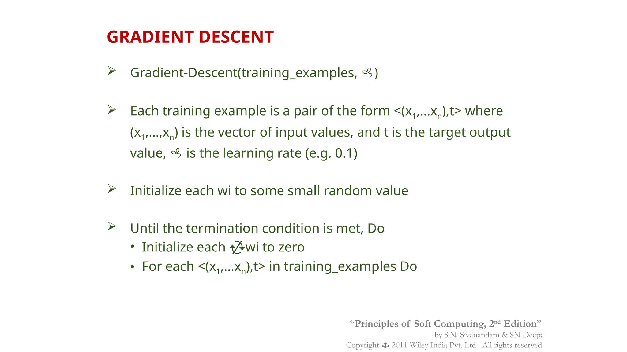
 Gradient-Descent(training_examples, )
 Each training example is a pair of the form <(x1,…xn),t> where
(x1,…,xn) is the vector of input values, and t is the target output
value,  is the learning rate (e.g. 0.1)
 Initialize each wi to some small random value
 Until the termination condition is met, Do
• Initialize each wi to zero
• For each <(x1,…xn),t> in training_examples Do
GRADIENT DESCENT
“Principles of Soft Computing, 2nd
Edition”
by S.N. Sivanandam & SN Deepa
Copyright  2011 Wiley India Pvt. Ltd. All rights reserved.
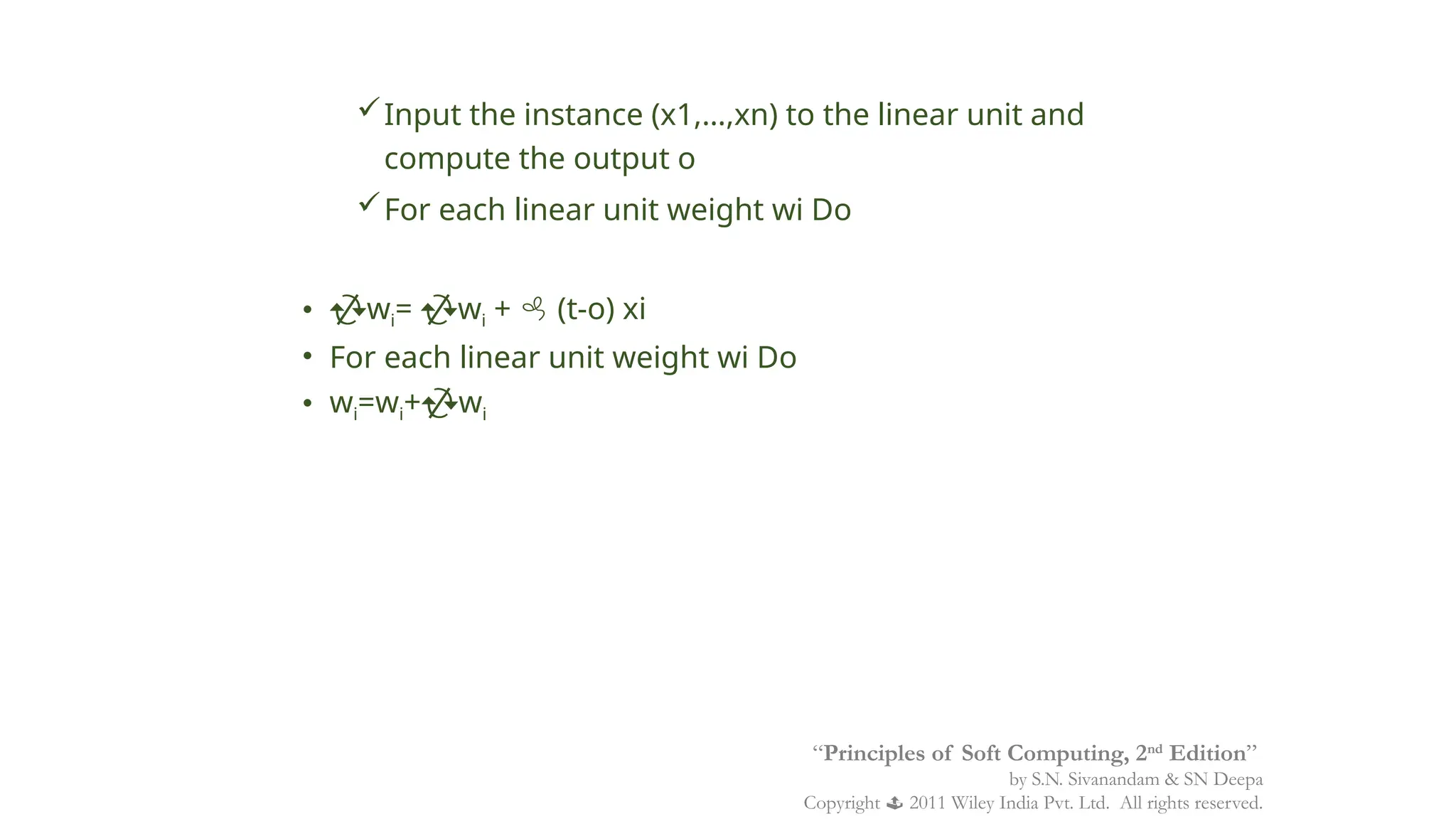
Input the instance (x1,…,xn) to the linear unit and
compute the output o
For each linear unit weight wi Do
• wi= wi +  (t-o) xi
• For each linear unit weight wi Do
• wi=wi+wi
“Principles of Soft Computing, 2nd
Edition”
by S.N. Sivanandam & SN Deepa
Copyright  2011 Wiley India Pvt. Ltd. All rights reserved.
 Batch mode : gradient descent
w=w -  ED[w] over the entire data D
ED[w]=1/2d(td-od)2
 Incremental mode: gradient descent
w=w -  Ed[w] over individual training examples
d
Ed[w]=1/2 (td-od)2
 Incremental Gradient Descent can approximate Batch Gradient
Descent arbitrarily closely if  is small enough.
MODES OF GRADIENT DESCENT
“Principles of Soft Computing, 2nd
Edition”
by S.N. Sivanandam & SN Deepa
Copyright  2011 Wiley India Pvt. Ltd. All rights reserved.
SIGMOID ACTIVATION FUNCTION

x1
x2
xn
.
.
.
w1
w2
wn
w0
x0=1
net=i=0
n
wi xi
o
o=(net)=1/(1+e-net
)
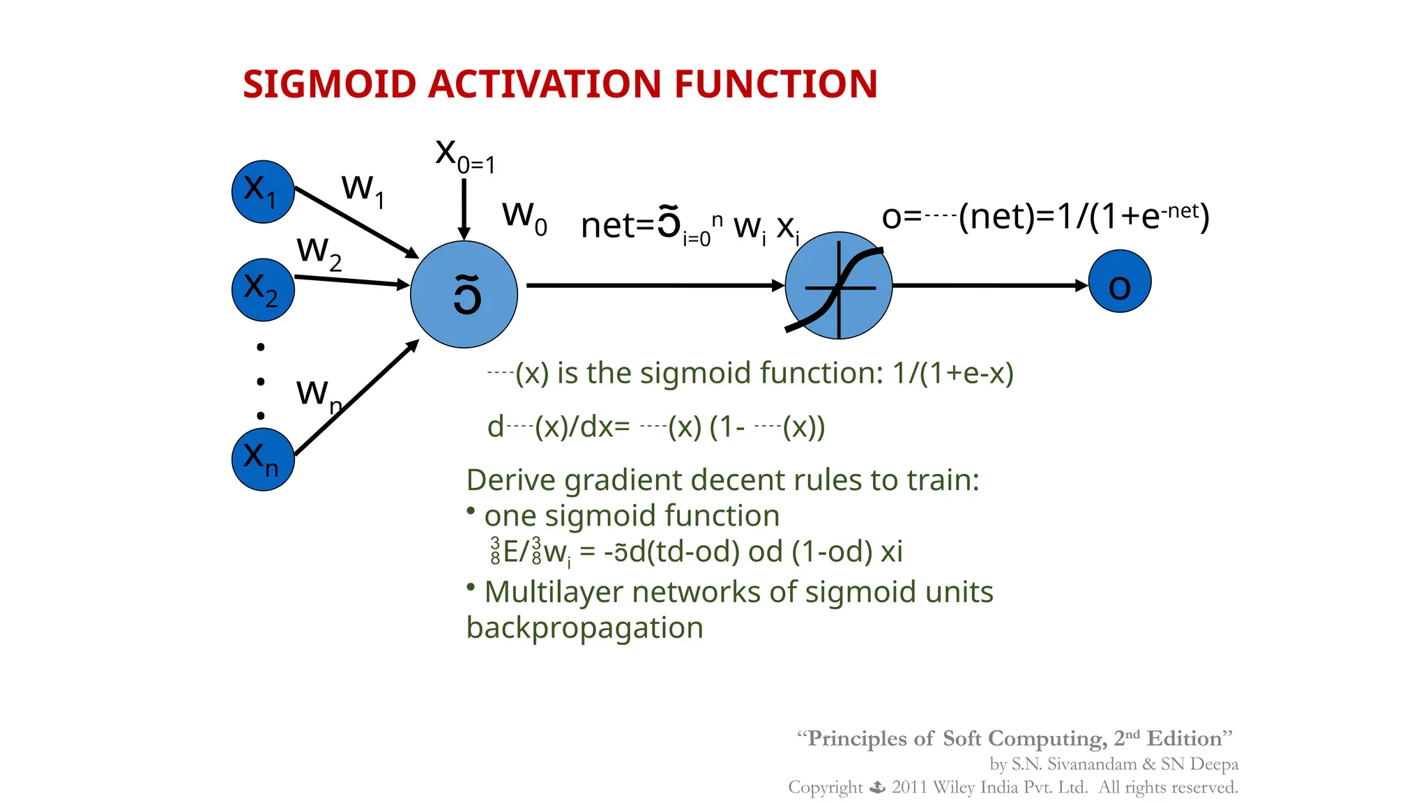
(x) is the sigmoid function: 1/(1+e-x)
d(x)/dx= (x) (1- (x))
Derive gradient decent rules to train:
• one sigmoid function
E/wi = -d(td-od) od (1-od) xi
• Multilayer networks of sigmoid units
backpropagation
“Principles of Soft Computing, 2nd
Edition”
by S.N. Sivanandam & SN Deepa
Copyright  2011 Wiley India Pvt. Ltd. All rights reserved.
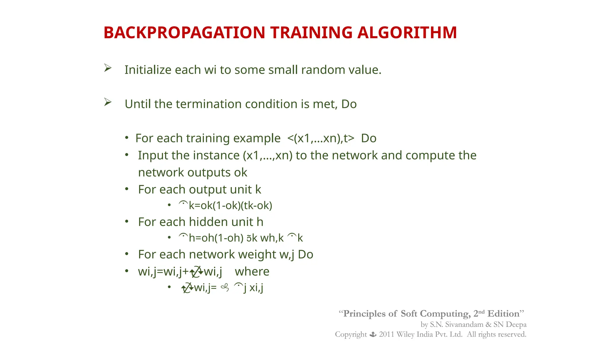
 Initialize each wi to some small random value.
 Until the termination condition is met, Do
• For each training example <(x1,…xn),t> Do
• Input the instance (x1,…,xn) to the network and compute the
network outputs ok
• For each output unit k
• k=ok(1-ok)(tk-ok)
• For each hidden unit h
• h=oh(1-oh) k wh,k k
• For each network weight w,j Do
• wi,j=wi,j+wi,j where
• wi,j=  j xi,j
BACKPROPAGATION TRAINING ALGORITHM
“Principles of Soft Computing, 2nd
Edition”
by S.N. Sivanandam & SN Deepa
Copyright  2011 Wiley India Pvt. Ltd. All rights reserved.
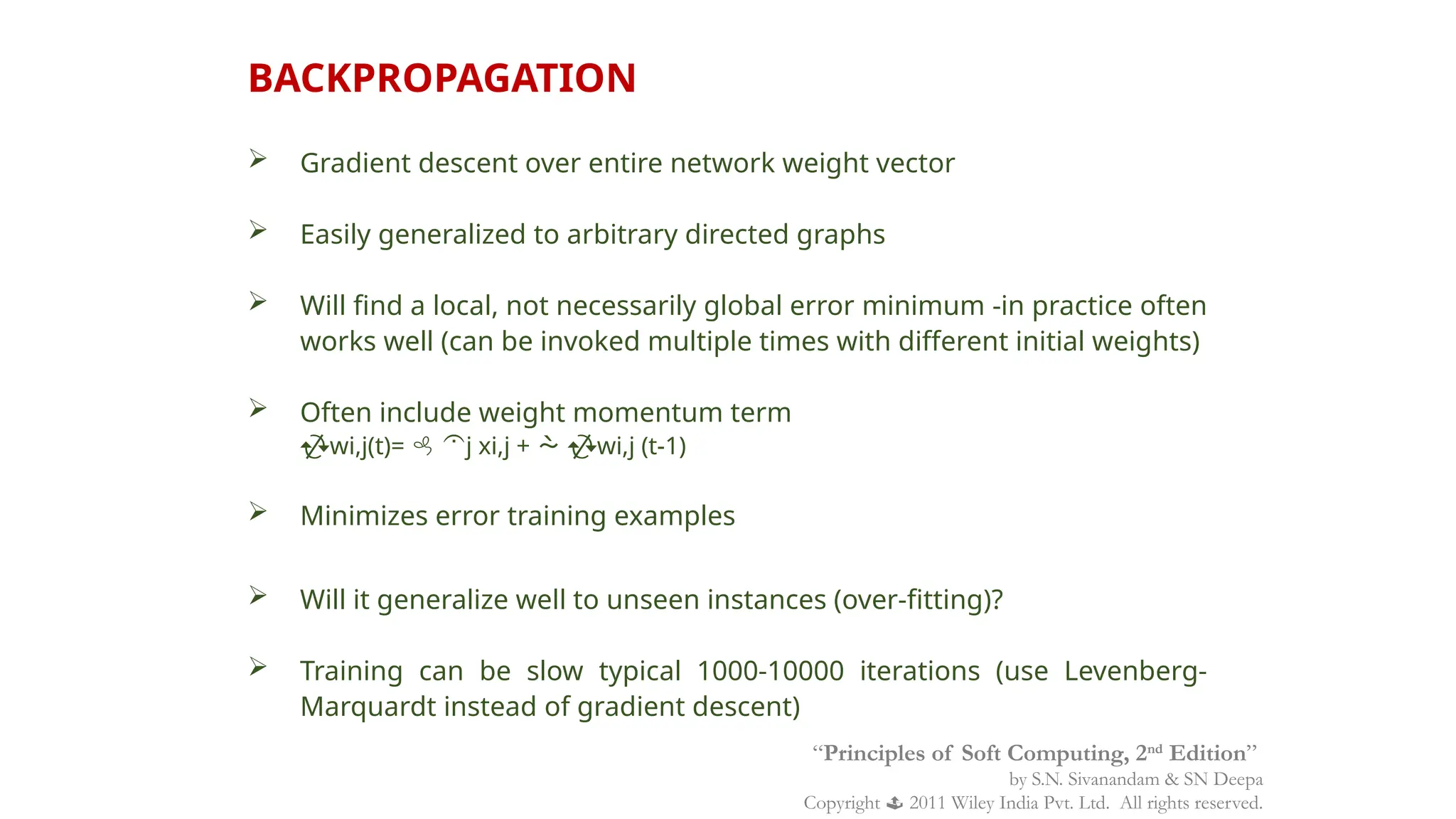
 Gradient descent over entire network weight vector
 Easily generalized to arbitrary directed graphs
 Will find a local, not necessarily global error minimum -in practice often
works well (can be invoked multiple times with different initial weights)
 Often include weight momentum term
wi,j(t)=  j xi,j +  wi,j (t-1)
 Minimizes error training examples
 Will it generalize well to unseen instances (over-fitting)?
 Training can be slow typical 1000-10000 iterations (use Levenberg-
Marquardt instead of gradient descent)
BACKPROPAGATION
“Principles of Soft Computing, 2nd
Edition”
by S.N. Sivanandam & SN Deepa
Copyright  2011 Wiley India Pvt. Ltd. All rights reserved.
APPLICATIONS OF BACKPROPAGATION
NETWORK
 Load forecasting problems in power systems.
 Image processing.
 Fault diagnosis and fault detection.
 Gesture recognition, speech recognition.
 Signature verification.
 Bioinformatics.
 Structural engineering design (civil).
“Principles of Soft Computing, 2nd
Edition”
by S.N. Sivanandam & SN Deepa
Copyright  2011 Wiley India Pvt. Ltd. All rights reserved.
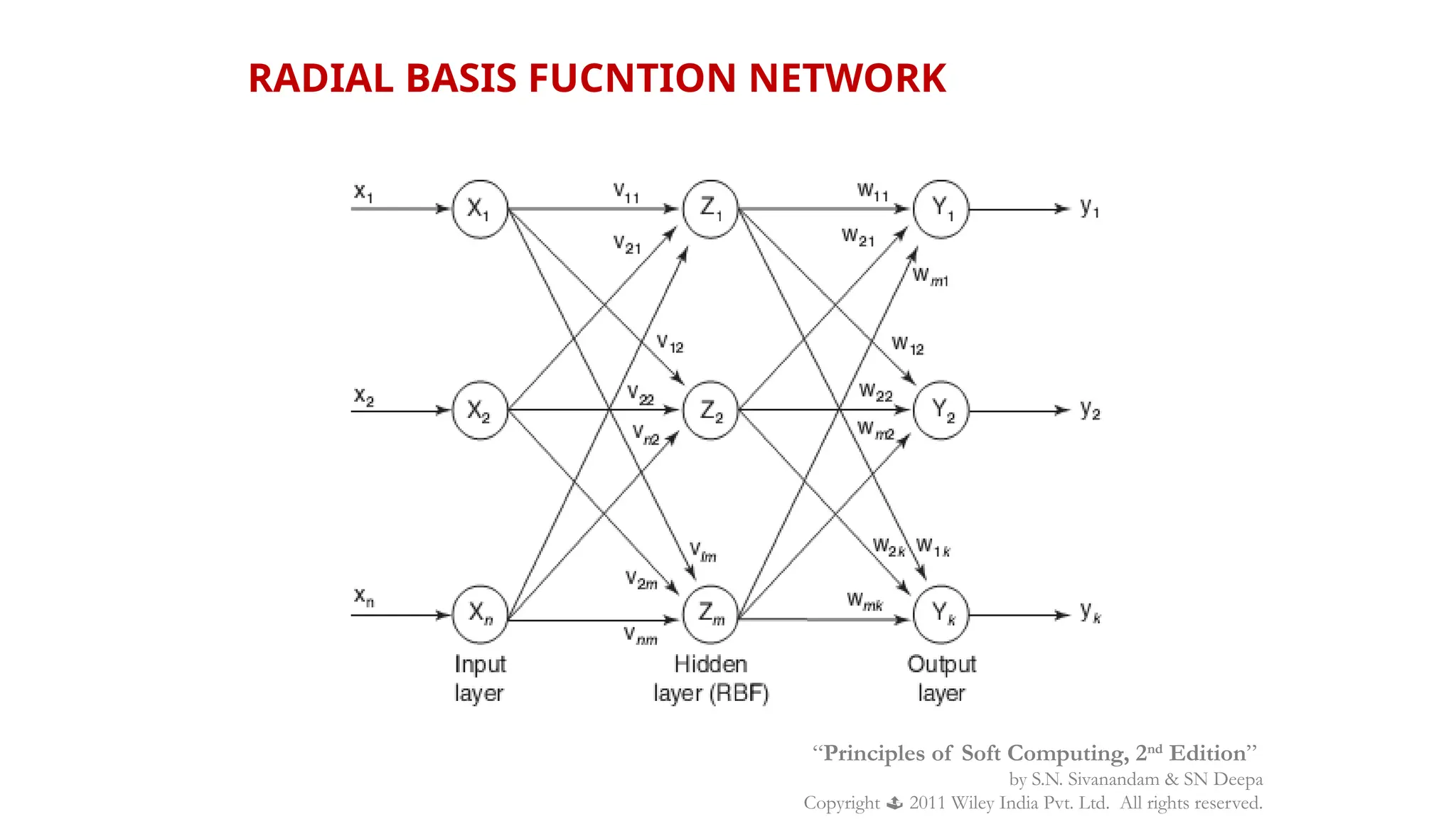
RADIAL BASIS FUCNTION NETWORK
 The radial basis function (RBF) is a classification and functional
approximation neural network developed by M.J.D. Powell.
 The network uses the most common nonlinearities such as
sigmoidal and Gaussian kernel functions.
 The Gaussian functions are also used in regularization
networks.
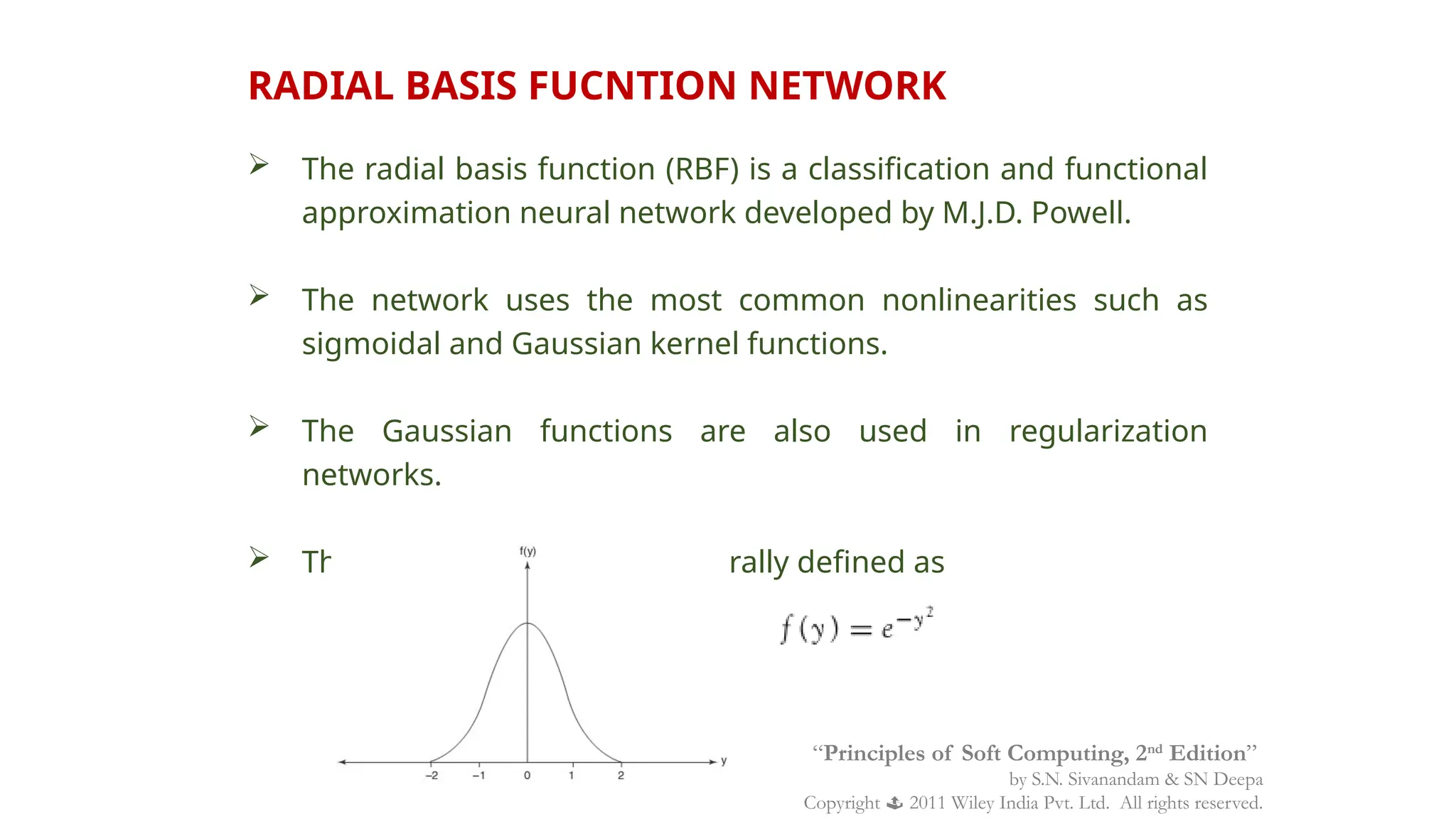
 The Gaussian function is generally defined as
“Principles of Soft Computing, 2nd
Edition”
by S.N. Sivanandam & SN Deepa
Copyright  2011 Wiley India Pvt. Ltd. All rights reserved.
RADIAL BASIS FUCNTION NETWORK
“Principles of Soft Computing, 2nd
Edition”
by S.N. Sivanandam & SN Deepa
Copyright  2011 Wiley India Pvt. Ltd. All rights reserved.
SUMMARY
This chapter discussed on the several supervised learning networks
like
 Perceptron,
 Adaline,
 Madaline,
 Backpropagation Network,
 Radial Basis Function Network.
Apart from these mentioned above, there are several other
supervised neural networks like tree neural networks, wavelet
neural network, functional link neural network and so on.
“Principles of Soft Computing, 2nd
Edition”
by S.N. Sivanandam & SN Deepa
Copyright  2011 Wiley India Pvt. Ltd. All rights reserved.

machine learning supervised learning with example

  • 1.
    CHAPTER 3 SUPERVISED LEARNING NETWORK “Principlesof Soft Computing, 2nd Edition” by S.N. Sivanandam & SN Deepa Copyright  2011 Wiley India Pvt. Ltd. All rights reserved.
  • 2.
    DEFINITION OF SUPERVISEDLEARNING NETWORKS  Training and test data sets  Training set; input & target are specified “Principles of Soft Computing, 2nd Edition” by S.N. Sivanandam & SN Deepa Copyright  2011 Wiley India Pvt. Ltd. All rights reserved.
  • 3.
    PERCEPTRON NETWORKS “Principles ofSoft Computing, 2nd Edition” by S.N. Sivanandam & SN Deepa Copyright  2011 Wiley India Pvt. Ltd. All rights reserved.
  • 4.
     Linear thresholdunit (LTU)  x1 x2 xn . . . w1 w2 wn w0  wi xi 1 if  wi xi >0 f(xi)= -1 otherwise o { n i=0 i=0 n “Principles of Soft Computing, 2nd Edition” by S.N. Sivanandam & SN Deepa Copyright  2011 Wiley India Pvt. Ltd. All rights reserved.
  • 5.
    PERCEPTRON LEARNING wi =wi + wi wi =  (t - o) xi where t = c(x) is the target value, o is the perceptron output,  Is a small constant (e.g., 0.1) called learning rate.  If the output is correct (t = o) the weights wi are not changed  If the output is incorrect (t  o) the weights wi are changed such that the output of the perceptron for the new weights is closer to t.  The algorithm converges to the correct classification • if the training data is linearly separable •  is sufficiently small “Principles of Soft Computing, 2nd Edition” by S.N. Sivanandam & SN Deepa Copyright  2011 Wiley India Pvt. Ltd. All rights reserved.
  • 6.
    LEARNING ALGORITHM  Epoch: Presentation of the entire training set to the neural network.  In the case of the AND function, an epoch consists of four sets of inputs being presented to the network (i.e. [0,0], [0,1], [1,0], [1,1]).  Error: The error value is the amount by which the value output by the network differs from the target value. For example, if we required the network to output 0 and it outputs 1, then Error = -1. “Principles of Soft Computing, 2nd Edition” by S.N. Sivanandam & SN Deepa Copyright  2011 Wiley India Pvt. Ltd. All rights reserved.
  • 7.
     Target Value,T : When we are training a network we not only present it with the input but also with a value that we require the network to produce. For example, if we present the network with [1,1] for the AND function, the training value will be 1.  Output , O : The output value from the neuron.  Ij : Inputs being presented to the neuron.  Wj : Weight from input neuron (Ij) to the output neuron.  LR : The learning rate. This dictates how quickly the network converges. It is set by a matter of experimentation. It is typically 0.1. “Principles of Soft Computing, 2nd Edition” by S.N. Sivanandam & SN Deepa Copyright  2011 Wiley India Pvt. Ltd. All rights reserved.
  • 8.
    TRAINING ALGORITHM  Adjustneural network weights to map inputs to outputs.  Use a set of sample patterns where the desired output (given the inputs presented) is known.  The purpose is to learn to • Recognize features which are common to good and bad exemplars “Principles of Soft Computing, 2nd Edition” by S.N. Sivanandam & SN Deepa Copyright  2011 Wiley India Pvt. Ltd. All rights reserved.
  • 9.
    MULTILAYER PERCEPTRON Output Values InputSignals (External Stimuli) Output Layer Adjustable Weights Input Layer “Principles of Soft Computing, 2nd Edition” by S.N. Sivanandam & SN Deepa Copyright  2011 Wiley India Pvt. Ltd. All rights reserved.
  • 10.
    LAYERS IN NEURALNETWORK  The input layer: • Introduces input values into the network. • No activation function or other processing.  The hidden layer(s): • Performs classification of features. • Two hidden layers are sufficient to solve any problem. • Features imply more layers may be better.  The output layer: • Functionally is just like the hidden layers. • Outputs are passed on to the world outside the neural network. “Principles of Soft Computing, 2nd Edition” by S.N. Sivanandam & SN Deepa Copyright  2011 Wiley India Pvt. Ltd. All rights reserved.
  • 11.
    ADAPTIVE LINEAR NEURON(ADALINE) In 1959, Bernard Widrow and Marcian Hoff of Stanford developed models they called ADALINE (Adaptive Linear Neuron) and MADALINE (Multilayer ADALINE). These models were named for their use of Multiple ADAptive LINear Elements. MADALINE was the first neural network to be applied to a real world problem. It is an adaptive filter which eliminates echoes on phone lines. “Principles of Soft Computing, 2nd Edition” by S.N. Sivanandam & SN Deepa Copyright  2011 Wiley India Pvt. Ltd. All rights reserved.
  • 12.
    ADALINE MODEL “Principles ofSoft Computing, 2nd Edition” by S.N. Sivanandam & SN Deepa Copyright  2011 Wiley India Pvt. Ltd. All rights reserved.
  • 13.
    ADALINE LEARNING RULE Adalinenetwork uses Delta Learning Rule. This rule is also called as Widrow Learning Rule or Least Mean Square Rule. The delta rule for adjusting the weights is given as (i = 1 to n): “Principles of Soft Computing, 2nd Edition” by S.N. Sivanandam & SN Deepa Copyright  2011 Wiley India Pvt. Ltd. All rights reserved.
  • 14.
    Initialize • Assign randomweights to all links Training • Feed-in known inputs in random sequence • Simulate the network • Compute error between the input and the output (Error Function) • Adjust weights (Learning Function) • Repeat until total error < ε Thinking • Simulate the network • Network will respond to any input • Does not guarantee a correct solution even for trained inputs USING ADALINE NETWORKS Initialize Training Thinking “Principles of Soft Computing, 2nd Edition” by S.N. Sivanandam & SN Deepa Copyright  2011 Wiley India Pvt. Ltd. All rights reserved.
  • 15.
    MADALINE NETWORK MADALINE isa Multilayer Adaptive Linear Element. MADALINE was the first neural network to be applied to a real world problem. It is used in several adaptive filtering process. “Principles of Soft Computing, 2nd Edition” by S.N. Sivanandam & SN Deepa Copyright  2011 Wiley India Pvt. Ltd. All rights reserved.
  • 16.
    BACK PROPAGATION NETWORK “Principlesof Soft Computing, 2nd Edition” by S.N. Sivanandam & SN Deepa Copyright  2011 Wiley India Pvt. Ltd. All rights reserved.
  • 17.
     A trainingprocedure which allows multilayer feed forward Neural Networks to be trained.  Can theoretically perform “any” input-output mapping.  Can learn to solve linearly inseparable problems. “Principles of Soft Computing, 2nd Edition” by S.N. Sivanandam & SN Deepa Copyright  2011 Wiley India Pvt. Ltd. All rights reserved.
  • 18.
    MULTILAYER FEEDFORWARD NETWORK Inputs Hiddens Outputs I1 I2 I3 I0 h0 h1 h2 o0 o1 Inputs Hiddens Outputs “Principlesof Soft Computing, 2nd Edition” by S.N. Sivanandam & SN Deepa Copyright  2011 Wiley India Pvt. Ltd. All rights reserved.
  • 19.
    MULTILAYER FEEDFORWARD NETWORK: ACTIVATIONAND TRAINING  For feed forward networks: • A continuous function can be • differentiated allowing • gradient-descent. • Back propagation is an example of a gradient-descent technique. • Uses sigmoid (binary or bipolar) activation function. “Principles of Soft Computing, 2nd Edition” by S.N. Sivanandam & SN Deepa Copyright  2011 Wiley India Pvt. Ltd. All rights reserved.
  • 20.
    In multilayer networks,the activation function is usually more complex than just a threshold function, like 1/[1+exp(-x)] or even 2/[1+exp(-x)] – 1 to allow for inhibition, etc. “Principles of Soft Computing, 2nd Edition” by S.N. Sivanandam & SN Deepa Copyright  2011 Wiley India Pvt. Ltd. All rights reserved.
  • 21.
     Gradient-Descent(training_examples, ) Each training example is a pair of the form <(x1,…xn),t> where (x1,…,xn) is the vector of input values, and t is the target output value,  is the learning rate (e.g. 0.1)  Initialize each wi to some small random value  Until the termination condition is met, Do • Initialize each wi to zero • For each <(x1,…xn),t> in training_examples Do GRADIENT DESCENT “Principles of Soft Computing, 2nd Edition” by S.N. Sivanandam & SN Deepa Copyright  2011 Wiley India Pvt. Ltd. All rights reserved.
  • 22.
    Input the instance(x1,…,xn) to the linear unit and compute the output o For each linear unit weight wi Do • wi= wi +  (t-o) xi • For each linear unit weight wi Do • wi=wi+wi “Principles of Soft Computing, 2nd Edition” by S.N. Sivanandam & SN Deepa Copyright  2011 Wiley India Pvt. Ltd. All rights reserved.
  • 23.
     Batch mode: gradient descent w=w -  ED[w] over the entire data D ED[w]=1/2d(td-od)2  Incremental mode: gradient descent w=w -  Ed[w] over individual training examples d Ed[w]=1/2 (td-od)2  Incremental Gradient Descent can approximate Batch Gradient Descent arbitrarily closely if  is small enough. MODES OF GRADIENT DESCENT “Principles of Soft Computing, 2nd Edition” by S.N. Sivanandam & SN Deepa Copyright  2011 Wiley India Pvt. Ltd. All rights reserved.
  • 24.
    SIGMOID ACTIVATION FUNCTION  x1 x2 xn . . . w1 w2 wn w0 x0=1 net=i=0 n wixi o o=(net)=1/(1+e-net ) (x) is the sigmoid function: 1/(1+e-x) d(x)/dx= (x) (1- (x)) Derive gradient decent rules to train: • one sigmoid function E/wi = -d(td-od) od (1-od) xi • Multilayer networks of sigmoid units backpropagation “Principles of Soft Computing, 2nd Edition” by S.N. Sivanandam & SN Deepa Copyright  2011 Wiley India Pvt. Ltd. All rights reserved.
  • 25.
     Initialize eachwi to some small random value.  Until the termination condition is met, Do • For each training example <(x1,…xn),t> Do • Input the instance (x1,…,xn) to the network and compute the network outputs ok • For each output unit k • k=ok(1-ok)(tk-ok) • For each hidden unit h • h=oh(1-oh) k wh,k k • For each network weight w,j Do • wi,j=wi,j+wi,j where • wi,j=  j xi,j BACKPROPAGATION TRAINING ALGORITHM “Principles of Soft Computing, 2nd Edition” by S.N. Sivanandam & SN Deepa Copyright  2011 Wiley India Pvt. Ltd. All rights reserved.
  • 26.
     Gradient descentover entire network weight vector  Easily generalized to arbitrary directed graphs  Will find a local, not necessarily global error minimum -in practice often works well (can be invoked multiple times with different initial weights)  Often include weight momentum term wi,j(t)=  j xi,j +  wi,j (t-1)  Minimizes error training examples  Will it generalize well to unseen instances (over-fitting)?  Training can be slow typical 1000-10000 iterations (use Levenberg- Marquardt instead of gradient descent) BACKPROPAGATION “Principles of Soft Computing, 2nd Edition” by S.N. Sivanandam & SN Deepa Copyright  2011 Wiley India Pvt. Ltd. All rights reserved.
  • 27.
    APPLICATIONS OF BACKPROPAGATION NETWORK Load forecasting problems in power systems.  Image processing.  Fault diagnosis and fault detection.  Gesture recognition, speech recognition.  Signature verification.  Bioinformatics.  Structural engineering design (civil). “Principles of Soft Computing, 2nd Edition” by S.N. Sivanandam & SN Deepa Copyright  2011 Wiley India Pvt. Ltd. All rights reserved.
  • 28.
    RADIAL BASIS FUCNTIONNETWORK  The radial basis function (RBF) is a classification and functional approximation neural network developed by M.J.D. Powell.  The network uses the most common nonlinearities such as sigmoidal and Gaussian kernel functions.  The Gaussian functions are also used in regularization networks.  The Gaussian function is generally defined as “Principles of Soft Computing, 2nd Edition” by S.N. Sivanandam & SN Deepa Copyright  2011 Wiley India Pvt. Ltd. All rights reserved.
  • 29.
    RADIAL BASIS FUCNTIONNETWORK “Principles of Soft Computing, 2nd Edition” by S.N. Sivanandam & SN Deepa Copyright  2011 Wiley India Pvt. Ltd. All rights reserved.
  • 30.
    SUMMARY This chapter discussedon the several supervised learning networks like  Perceptron,  Adaline,  Madaline,  Backpropagation Network,  Radial Basis Function Network. Apart from these mentioned above, there are several other supervised neural networks like tree neural networks, wavelet neural network, functional link neural network and so on. “Principles of Soft Computing, 2nd Edition” by S.N. Sivanandam & SN Deepa Copyright  2011 Wiley India Pvt. Ltd. All rights reserved.