Department of Information Technology 1Soft Computing (ITC4256 )
Supervised learning network
Dr. C.V. Suresh Babu
Professor
Department of IT
Hindustan Institute of Science & Technology
Department of Information Technology 2Soft Computing (ITC4256 )
Discussion Topics
• Supervised Learning Networks
- Perceptron networks
- Perceptron network- training algorithm
• Quiz at the end of session.
Department of Information Technology 3Soft Computing (ITC4256 )
Introduction
Department of Information Technology 4Soft Computing (ITC4256 )
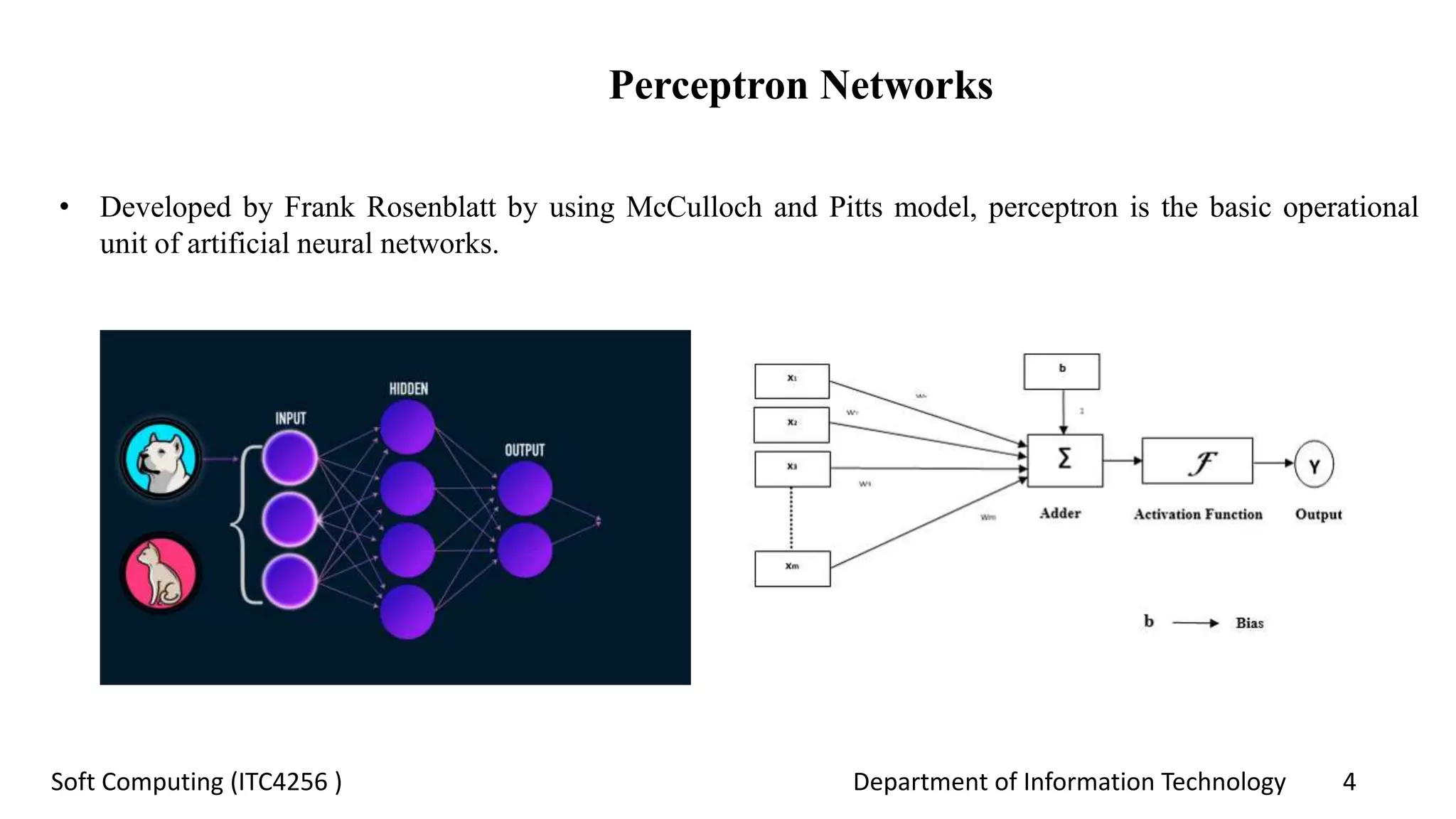
Perceptron Networks
• Developed by Frank Rosenblatt by using McCulloch and Pitts model, perceptron is the basic operational
unit of artificial neural networks.
Department of Information Technology 5Soft Computing (ITC4256 )
Perceptron Networks (Cont…)
• Perceptron thus has the following three basic elements:
- Links
- Adder
- Activation function
• Perceptron network can be trained for single output unit as well as multiple output units.
Department of Information Technology 6Soft Computing (ITC4256 )
Department of Information Technology 7Soft Computing (ITC4256 )
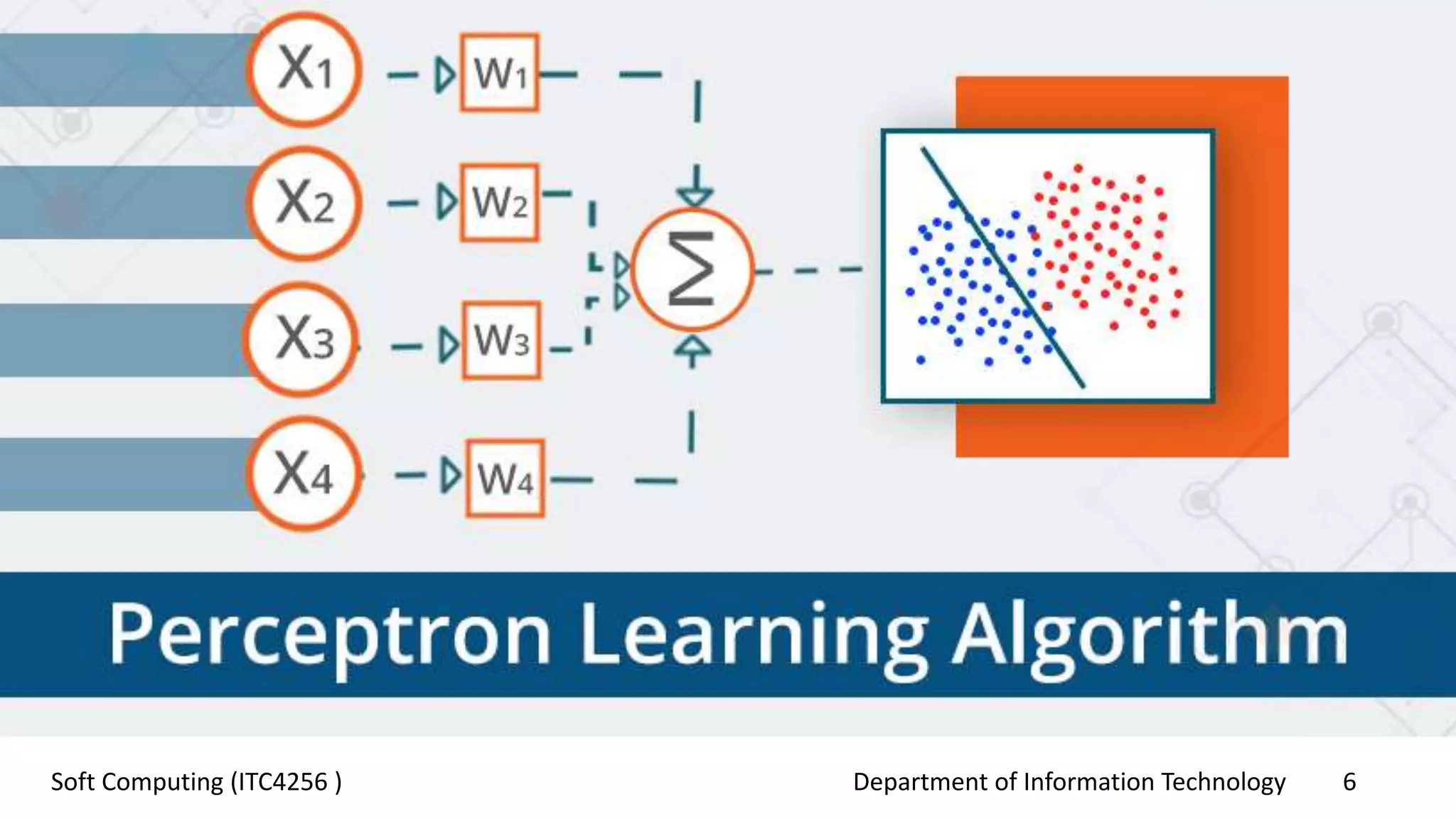
Perceptron Networks – Training Algorithm
Training Algorithm for Single Output Unit:
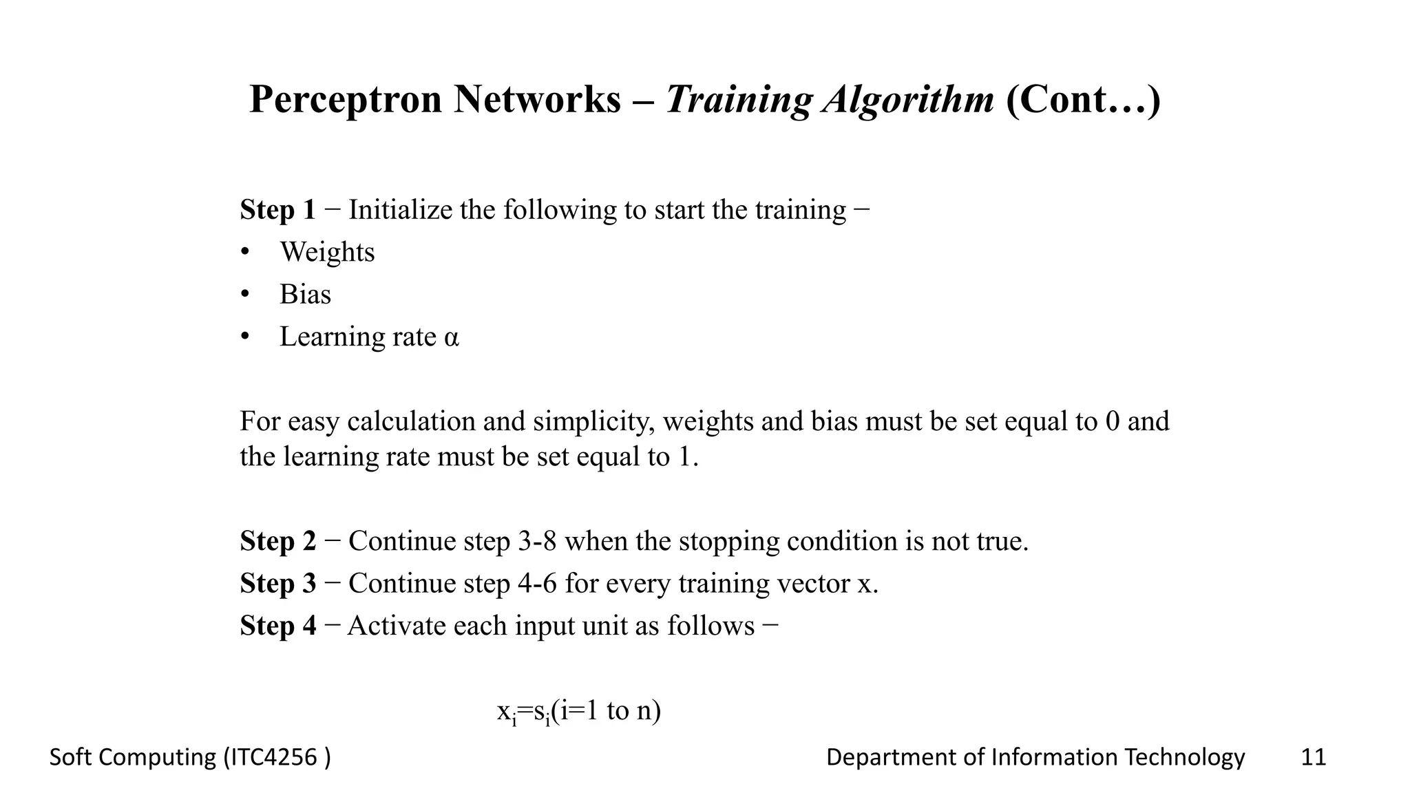
Step 1 − Initialize the following to start the training −
• Weights
• Bias
• Learning rate α
For easy calculation and simplicity, weights and bias must be set equal to 0 and
the learning rate must be set equal to 1.
Step 2 − Continue step 3-8 when the stopping condition is not true.
Step 3 − Continue step 4-6 for every training vector x.
Step 4 − Activate each input unit as follows −
xi=si(i=1 to n)
Department of Information Technology 8Soft Computing (ITC4256 )
Perceptron Networks – Training Algorithm (Cont…)
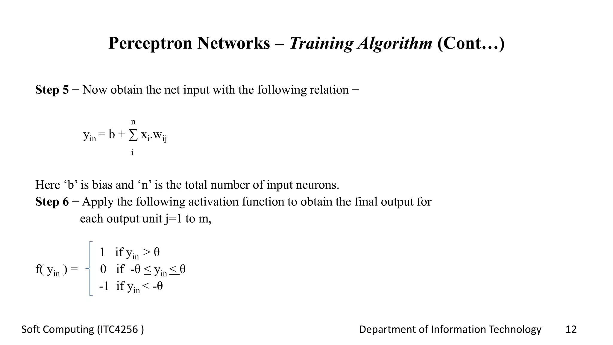
Step 5 − Now obtain the net input with the following relation −
n
yin = b + ∑ xi.wi
i
Here ‘b’ is bias and ‘n’ is the total number of input neurons.
Step 6 − Apply the following activation function to obtain the final output.
1 if yin > θ
f( yin ) = 0 if -θ < yin < θ
-1 if yin < -θ
Department of Information Technology 9Soft Computing (ITC4256 )
Perceptron Networks – Training Algorithm (Cont…)
Step 7 − Adjust the weight and bias as follows −
Case 1 − if y ≠ t then,
wi(new)=wi(old)+α txi
b(new)=b(old)+αt
Case 2 − if y = t then,
wi(new)=wi(old)
b(new)=b(old)
Here ‘y’ is the actual output and ‘t’ is the desired/target output.
Step 8 − Test for the stopping condition, which would happen when there is no
change in weight.
Department of Information Technology 10Soft Computing (ITC4256 )
Perceptron Networks – Training Algorithm (Cont…)
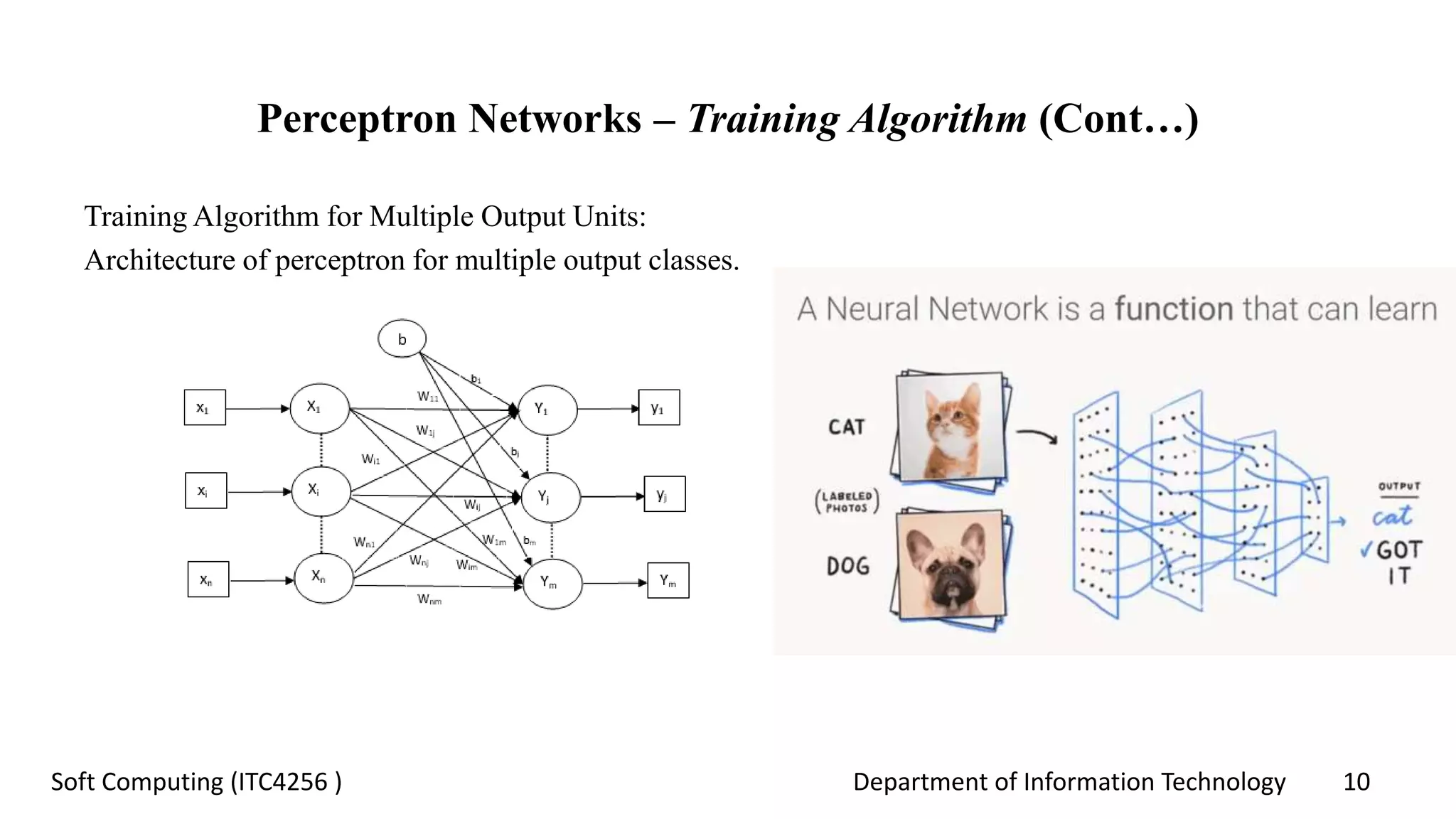
Training Algorithm for Multiple Output Units:
Architecture of perceptron for multiple output classes.
Department of Information Technology 11Soft Computing (ITC4256 )
Perceptron Networks – Training Algorithm (Cont…)
Step 1 − Initialize the following to start the training −
• Weights
• Bias
• Learning rate α
For easy calculation and simplicity, weights and bias must be set equal to 0 and
the learning rate must be set equal to 1.
Step 2 − Continue step 3-8 when the stopping condition is not true.
Step 3 − Continue step 4-6 for every training vector x.
Step 4 − Activate each input unit as follows −
xi=si(i=1 to n)
Department of Information Technology 12Soft Computing (ITC4256 )
Perceptron Networks – Training Algorithm (Cont…)
Step 5 − Now obtain the net input with the following relation −
n
yin = b + ∑ xi.wij
i
Here ‘b’ is bias and ‘n’ is the total number of input neurons.
Step 6 − Apply the following activation function to obtain the final output for
each output unit j=1 to m,
1 if yin > θ
f( yin ) = 0 if -θ < yin < θ
-1 if yin < -θ
Department of Information Technology 13Soft Computing (ITC4256 )
Perceptron Networks – Training Algorithm (Cont…)
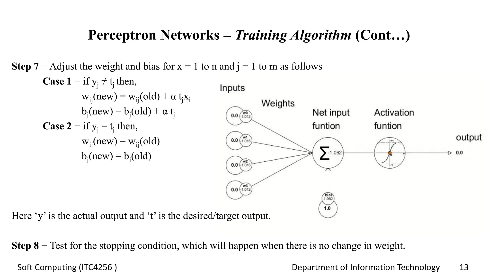
Step 7 − Adjust the weight and bias for x = 1 to n and j = 1 to m as follows −
Case 1 − if yj ≠ tj then,
wij(new) = wij(old) + α tjxi
bj(new) = bj(old) + α tj
Case 2 − if yj = tj then,
wij(new) = wij(old)
bj(new) = bj(old)
Here ‘y’ is the actual output and ‘t’ is the desired/target output.
Step 8 − Test for the stopping condition, which will happen when there is no change in weight.
Department of Information Technology 14Soft Computing (ITC4256 )
Quiz - Questions
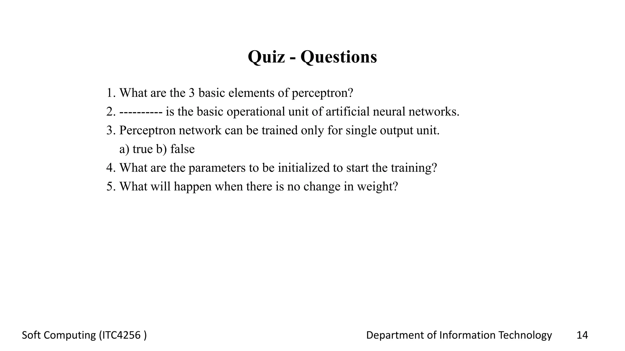
1. What are the 3 basic elements of perceptron?
2. ---------- is the basic operational unit of artificial neural networks.
3. Perceptron network can be trained only for single output unit.
a) true b) false
4. What are the parameters to be initialized to start the training?
5. What will happen when there is no change in weight?
Department of Information Technology 15Soft Computing (ITC4256 )
Quiz - Answers
1. What are the 3 basic elements of perceptron?
i. links ii. adder iii. activation function
2. ---------- is the basic operational unit of artificial neural networks.
Perceptron
3. Perceptron network can be trained only for single output unit.
b) false
4. Weights, bias and learning rate α
5. Stopping condition
Department of Information Technology 16Soft Computing (ITC4256 )
Action Plan
• Supervised Learning Networks (Cont…)
- Introduction to adaptive linear neuron
- Adaptive linear neuron architecture
- Adaptive linear neuron training algorithm
- Introduction to multiple adaptive linear neuron
- Multiple adaptive linear neuron architecture
- Multiple adaptive linear neuron training algorithm
• Quiz at the end of session.
Department of Information Technology 17Soft Computing (ITC4256 )
Adaptive Linear Neuron
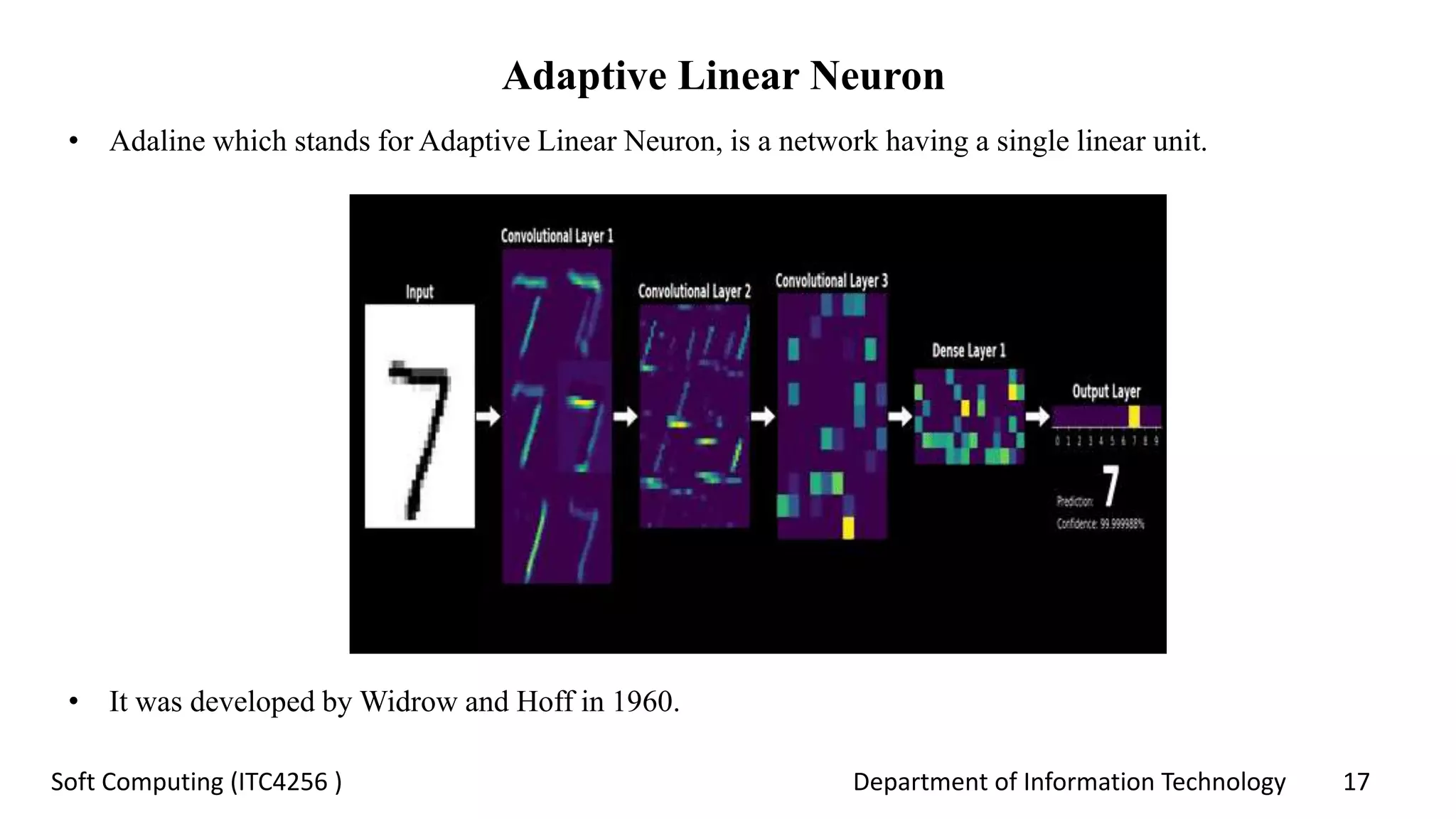
• Adaline which stands for Adaptive Linear Neuron, is a network having a single linear unit.
• It was developed by Widrow and Hoff in 1960.
Department of Information Technology 18Soft Computing (ITC4256 )
Adaptive Linear Neuron - Architecture
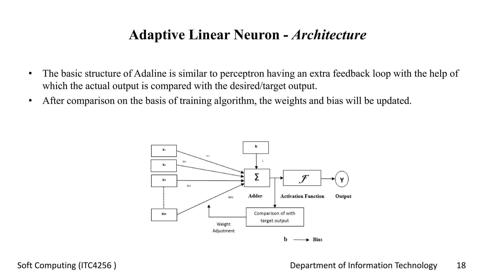
• The basic structure of Adaline is similar to perceptron having an extra feedback loop with the help of
which the actual output is compared with the desired/target output.
• After comparison on the basis of training algorithm, the weights and bias will be updated.
Department of Information Technology 19Soft Computing (ITC4256 )
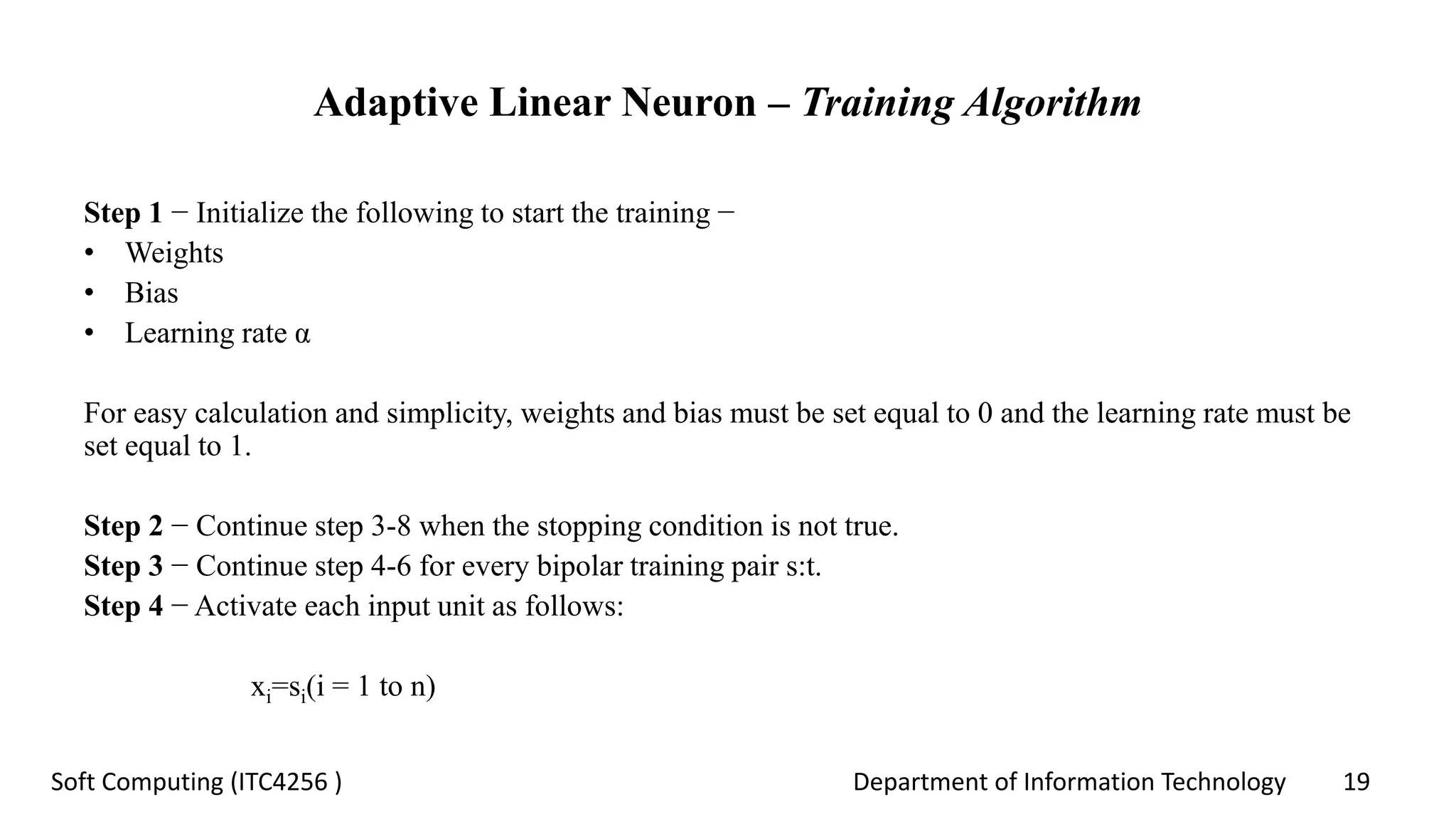
Adaptive Linear Neuron – Training Algorithm
Step 1 − Initialize the following to start the training −
• Weights
• Bias
• Learning rate α
For easy calculation and simplicity, weights and bias must be set equal to 0 and the learning rate must be
set equal to 1.
Step 2 − Continue step 3-8 when the stopping condition is not true.
Step 3 − Continue step 4-6 for every bipolar training pair s:t.
Step 4 − Activate each input unit as follows:
xi=si(i = 1 to n)
Department of Information Technology 20Soft Computing (ITC4256 )
Adaptive Linear Neuron – Training Algorithm
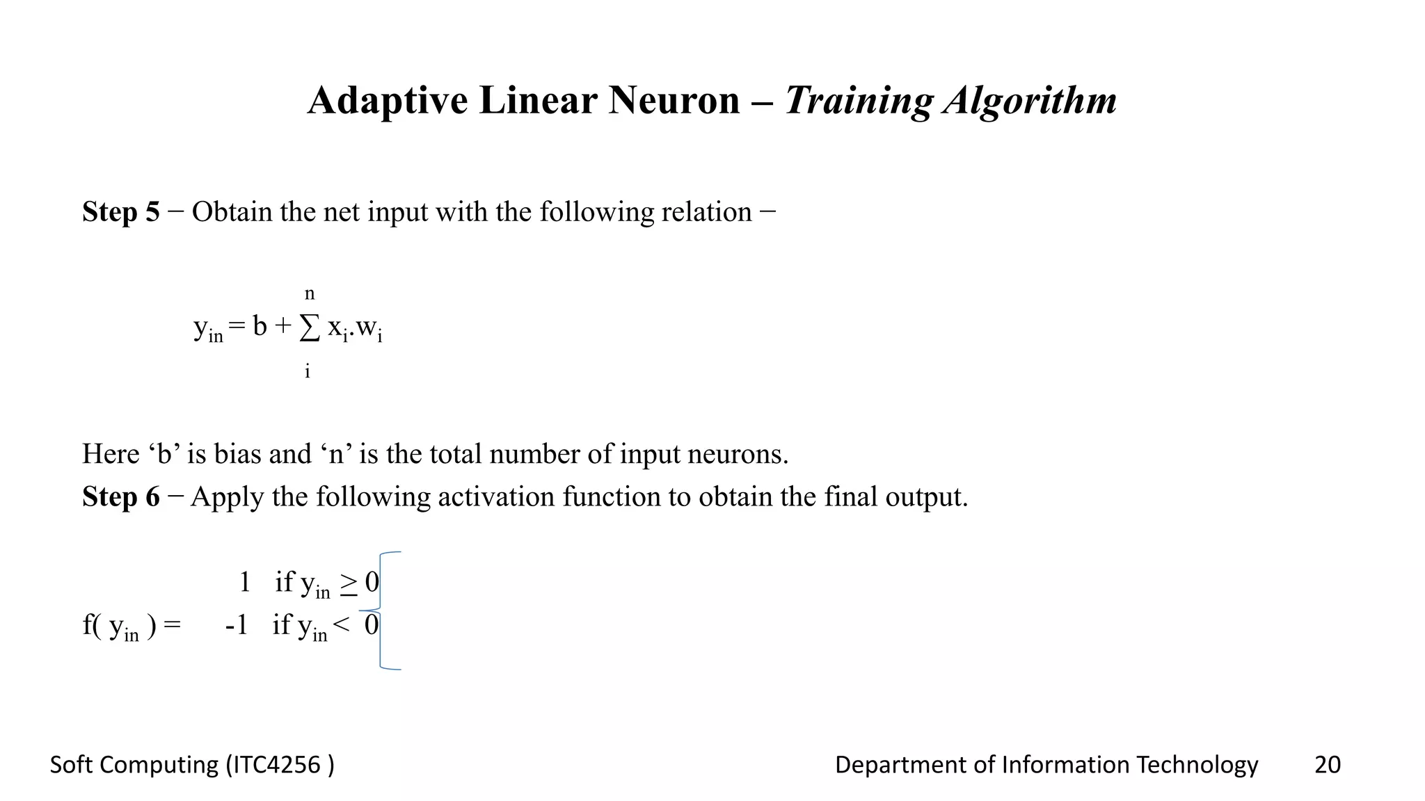
Step 5 − Obtain the net input with the following relation −
n
yin = b + ∑ xi.wi
i
Here ‘b’ is bias and ‘n’ is the total number of input neurons.
Step 6 − Apply the following activation function to obtain the final output.
1 if yin > 0
f( yin ) = -1 if yin < 0
Department of Information Technology 21Soft Computing (ITC4256 )
Adaptive Linear Neuron – Training Algorithm
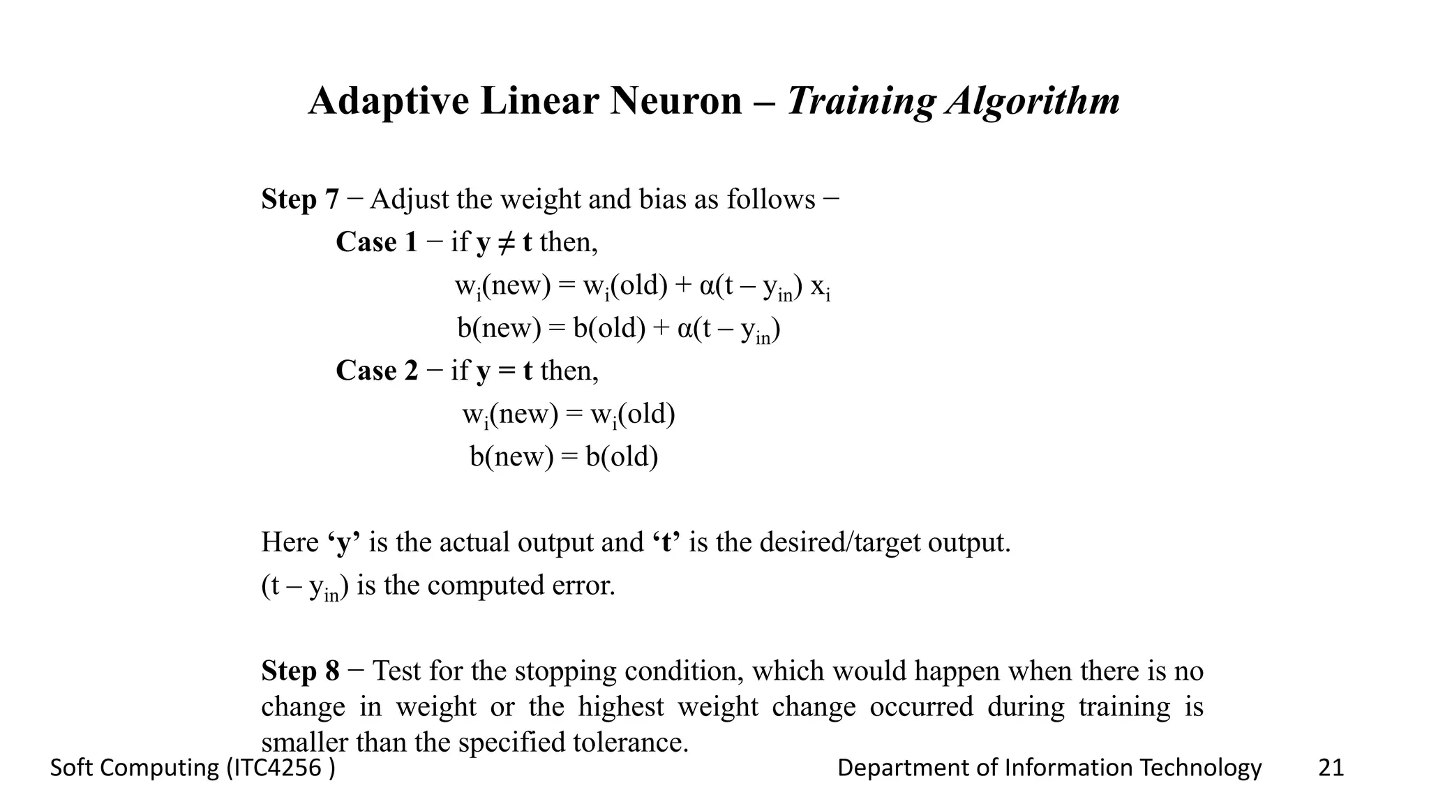
Step 7 − Adjust the weight and bias as follows −
Case 1 − if y ≠ t then,
wi(new) = wi(old) + α(t – yin) xi
b(new) = b(old) + α(t – yin)
Case 2 − if y = t then,
wi(new) = wi(old)
b(new) = b(old)
Here ‘y’ is the actual output and ‘t’ is the desired/target output.
(t – yin) is the computed error.
Step 8 − Test for the stopping condition, which would happen when there is no
change in weight or the highest weight change occurred during training is
smaller than the specified tolerance.
Department of Information Technology 22Soft Computing (ITC4256 )
Multiple Adaptive Linear Neuron
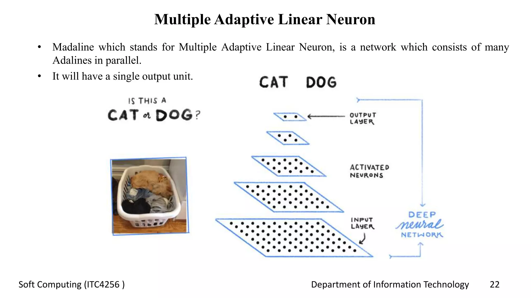
• Madaline which stands for Multiple Adaptive Linear Neuron, is a network which consists of many
Adalines in parallel.
• It will have a single output unit.
Department of Information Technology 23Soft Computing (ITC4256 )
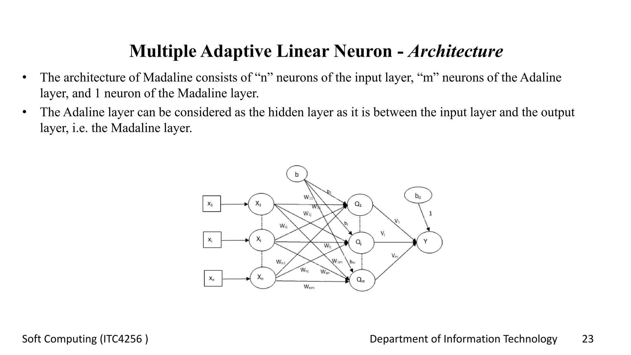
Multiple Adaptive Linear Neuron - Architecture
• The architecture of Madaline consists of “n” neurons of the input layer, “m” neurons of the Adaline
layer, and 1 neuron of the Madaline layer.
• The Adaline layer can be considered as the hidden layer as it is between the input layer and the output
layer, i.e. the Madaline layer.
Department of Information Technology 24Soft Computing (ITC4256 )
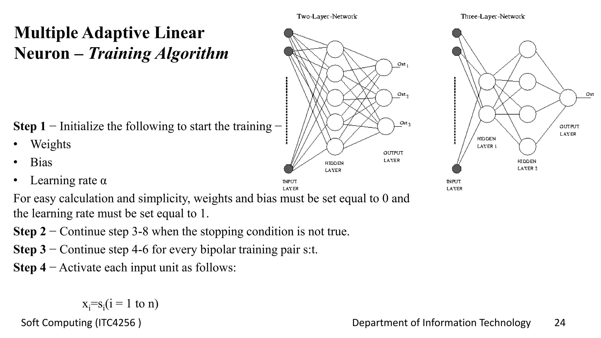
Multiple Adaptive Linear
Neuron – Training Algorithm
Step 1 − Initialize the following to start the training −
• Weights
• Bias
• Learning rate α
For easy calculation and simplicity, weights and bias must be set equal to 0 and
the learning rate must be set equal to 1.
Step 2 − Continue step 3-8 when the stopping condition is not true.
Step 3 − Continue step 4-6 for every bipolar training pair s:t.
Step 4 − Activate each input unit as follows:
xi=si(i = 1 to n)
Department of Information Technology 25Soft Computing (ITC4256 )
Multiple Adaptive Linear Neuron – Training Algorithm
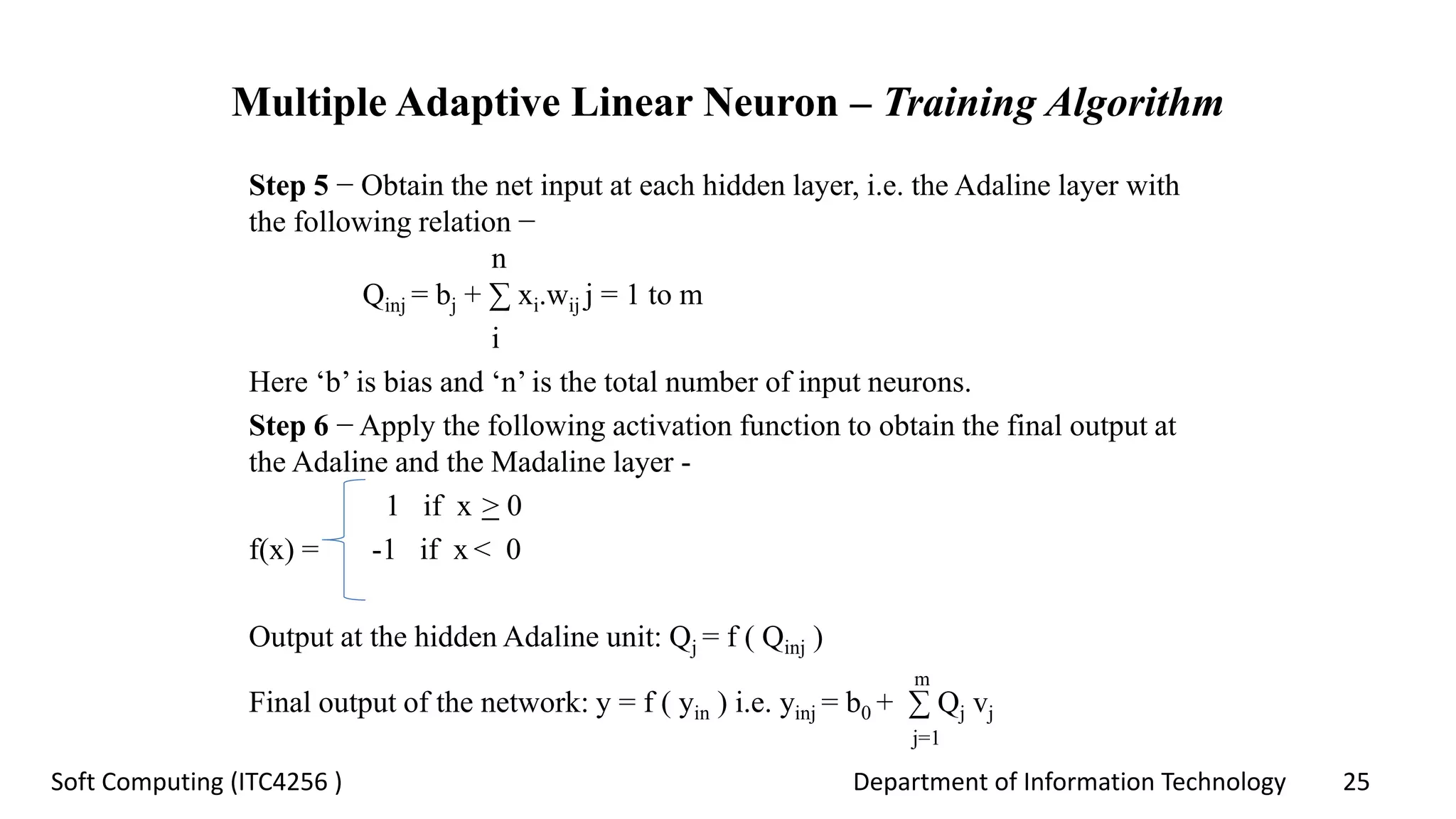
Step 5 − Obtain the net input at each hidden layer, i.e. the Adaline layer with
the following relation −
n
Qinj = bj + ∑ xi.wij j = 1 to m
i
Here ‘b’ is bias and ‘n’ is the total number of input neurons.
Step 6 − Apply the following activation function to obtain the final output at
the Adaline and the Madaline layer -
1 if x > 0
f(x) = -1 if x < 0
Output at the hidden Adaline unit: Qj = f ( Qinj )
m
Final output of the network: y = f ( yin ) i.e. yinj = b0 + ∑ Qj vj
j=1
Department of Information Technology 26Soft Computing (ITC4256 )
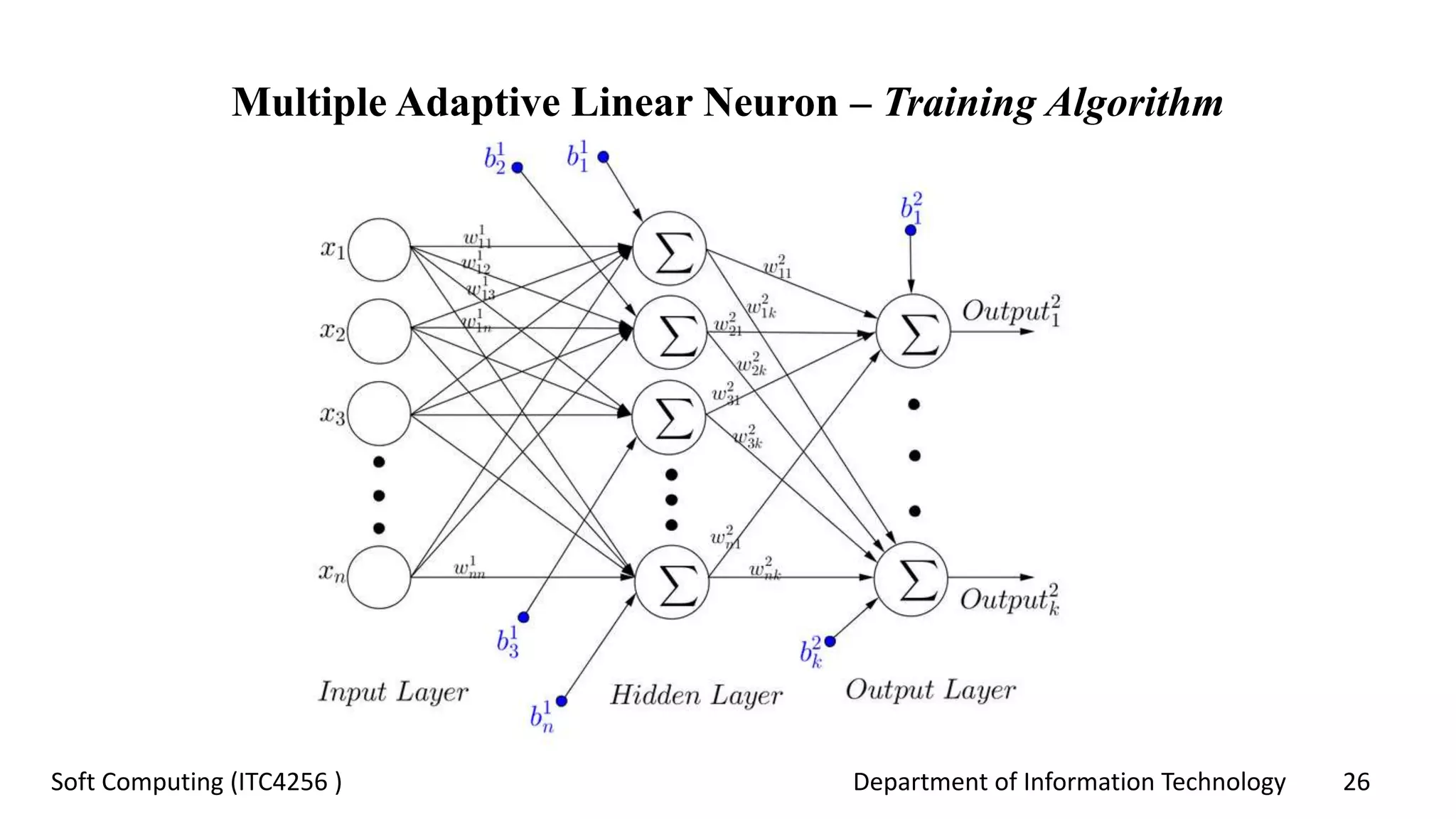
Multiple Adaptive Linear Neuron – Training Algorithm
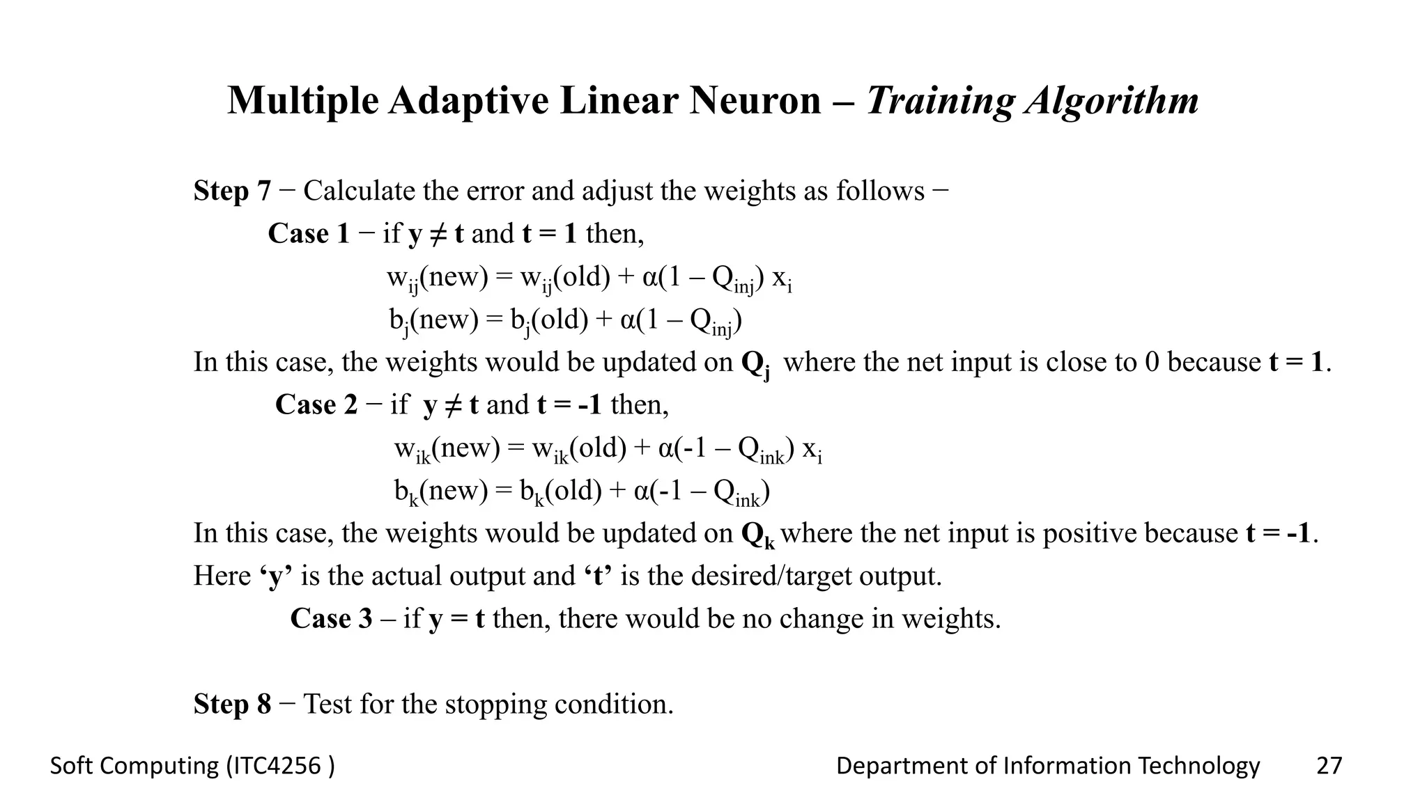
Department of Information Technology 27Soft Computing (ITC4256 )
Multiple Adaptive Linear Neuron – Training Algorithm
Step 7 − Calculate the error and adjust the weights as follows −
Case 1 − if y ≠ t and t = 1 then,
wij(new) = wij(old) + α(1 – Qinj) xi
bj(new) = bj(old) + α(1 – Qinj)
In this case, the weights would be updated on Qj where the net input is close to 0 because t = 1.
Case 2 − if y ≠ t and t = -1 then,
wik(new) = wik(old) + α(-1 – Qink) xi
bk(new) = bk(old) + α(-1 – Qink)
In this case, the weights would be updated on Qk where the net input is positive because t = -1.
Here ‘y’ is the actual output and ‘t’ is the desired/target output.
Case 3 – if y = t then, there would be no change in weights.
Step 8 − Test for the stopping condition.
Department of Information Technology 28Soft Computing (ITC4256 )
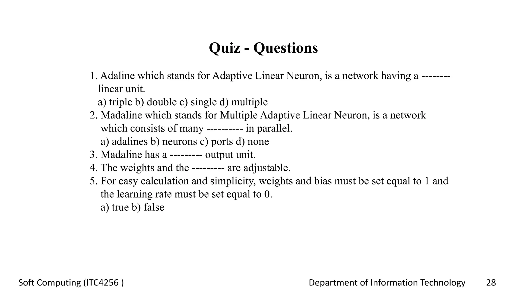
Quiz - Questions
1. Adaline which stands for Adaptive Linear Neuron, is a network having a --------
linear unit.
a) triple b) double c) single d) multiple
2. Madaline which stands for Multiple Adaptive Linear Neuron, is a network
which consists of many ---------- in parallel.
a) adalines b) neurons c) ports d) none
3. Madaline has a --------- output unit.
4. The weights and the --------- are adjustable.
5. For easy calculation and simplicity, weights and bias must be set equal to 1 and
the learning rate must be set equal to 0.
a) true b) false
Department of Information Technology 29Soft Computing (ITC4256 )
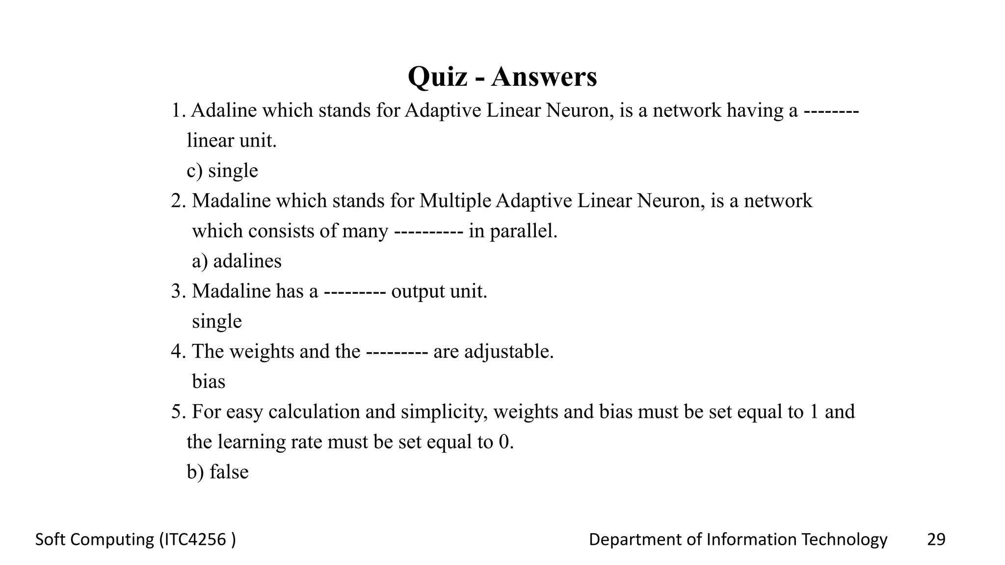
Quiz - Answers
1. Adaline which stands for Adaptive Linear Neuron, is a network having a --------
linear unit.
c) single
2. Madaline which stands for Multiple Adaptive Linear Neuron, is a network
which consists of many ---------- in parallel.
a) adalines
3. Madaline has a --------- output unit.
single
4. The weights and the --------- are adjustable.
bias
5. For easy calculation and simplicity, weights and bias must be set equal to 1 and
the learning rate must be set equal to 0.
b) false
Department of Information Technology 30Soft Computing (ITC4256 )
Action Plan
• Supervised Learning Networks (Cont…)
- Introduction to back propagation neural networks
- Back propagation network architecture
- Back propagation network training algorithm
- Generalized delta learning rule
• Quiz at the end of session
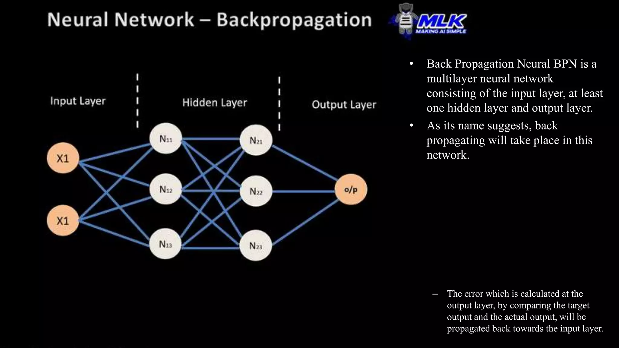
• Back Propagation Neural BPN is a
multilayer neural network
consisting of the input layer, at least
one hidden layer and output layer.
• As its name suggests, back
propagating will take place in this
network.
– The error which is calculated at the
output layer, by comparing the target
output and the actual output, will be
propagated back towards the input layer.
Department of Information Technology 32Soft Computing (ITC4256 )
Back Propagation Neural Networks - Architecture
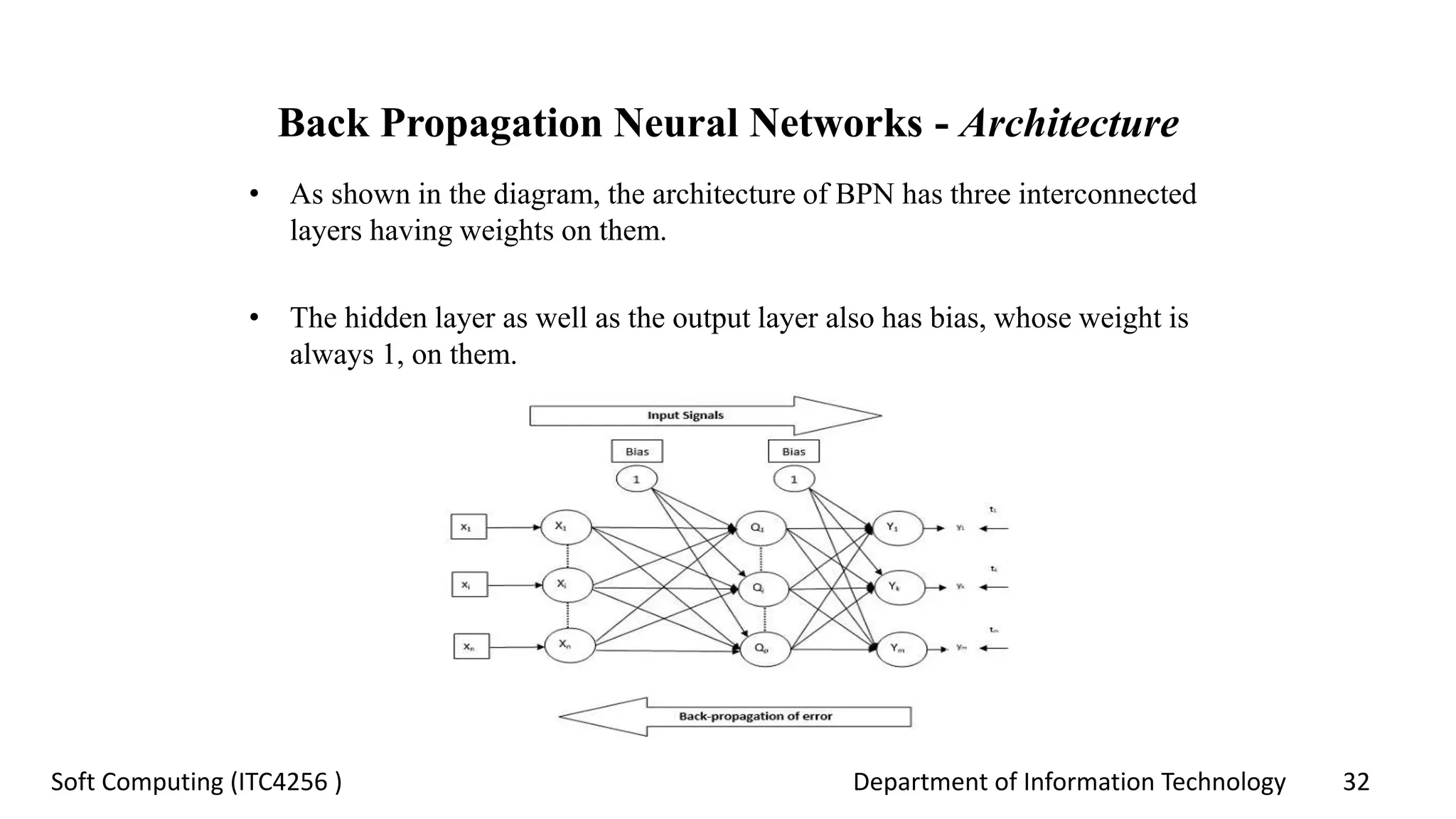
• As shown in the diagram, the architecture of BPN has three interconnected
layers having weights on them.
• The hidden layer as well as the output layer also has bias, whose weight is
always 1, on them.
Department of Information Technology 33Soft Computing (ITC4256 )
Back Propagation Neural Networks – Training Algorithm
For training, BPN will use binary sigmoid activation function. The training of BPN will have the
following three phases.
- Phase 1: Feed Forward Phase
- Phase 2: Back Propagation of error
- Phase 3: Updating of weights
All these steps will be concluded in the algorithm as follows
Step 1 − Initialize the following to start the training −
- Weights
- Learning rate α
For easy calculation and simplicity, take some small random values.
Step 2 − Continue step 3-11 when the stopping condition is not true.
Step 3 − Continue step 4-10 for every training pair.
Department of Information Technology 34Soft Computing (ITC4256 )
Back Propagation Neural Networks – Training Algorithm
Phase 1
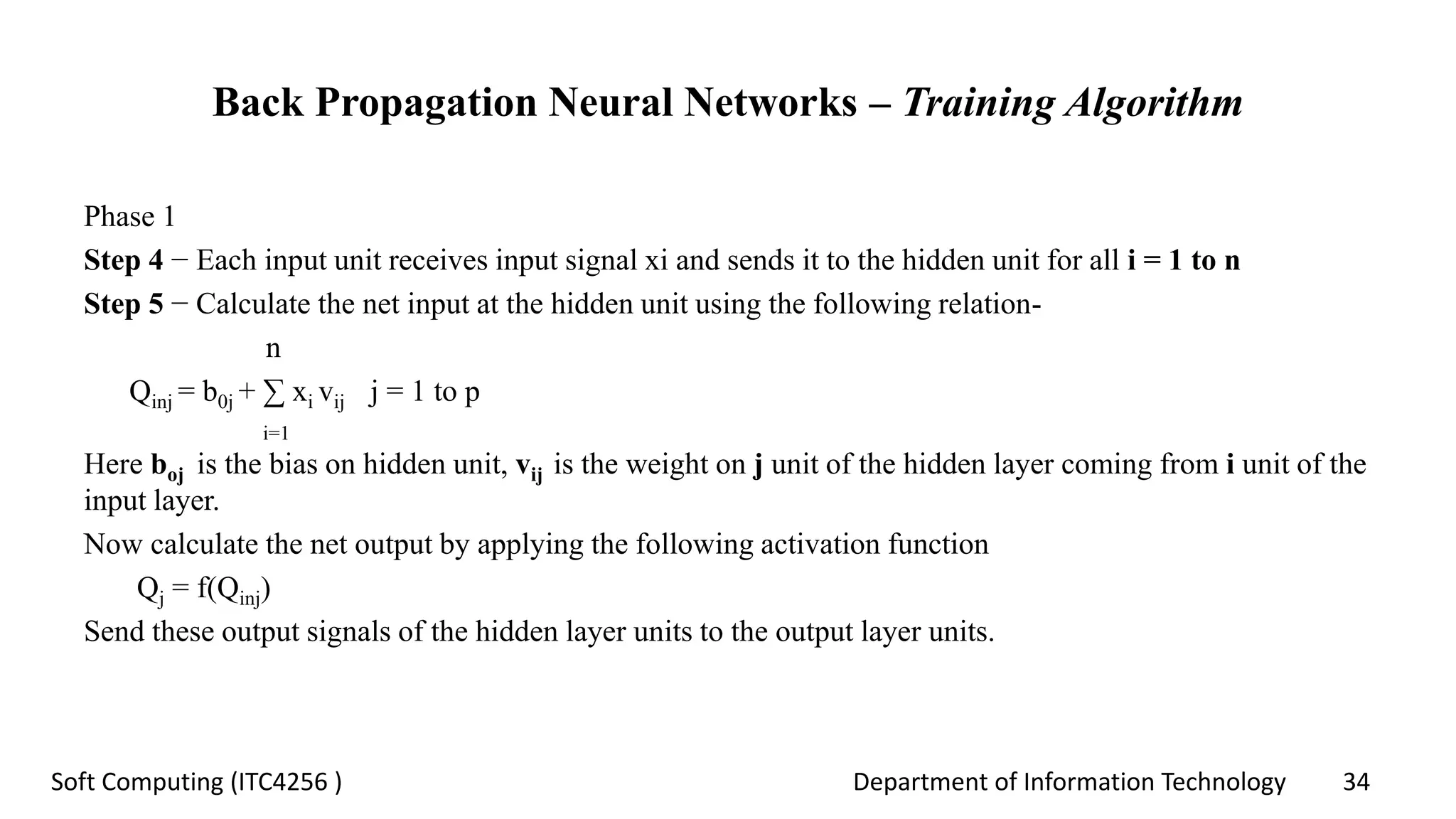
Step 4 − Each input unit receives input signal xi and sends it to the hidden unit for all i = 1 to n
Step 5 − Calculate the net input at the hidden unit using the following relation-
n
Qinj = b0j + ∑ xi vij j = 1 to p
i=1
Here boj is the bias on hidden unit, vij is the weight on j unit of the hidden layer coming from i unit of the
input layer.
Now calculate the net output by applying the following activation function
Qj = f(Qinj)
Send these output signals of the hidden layer units to the output layer units.
Department of Information Technology 35Soft Computing (ITC4256 )
Back Propagation Neural Networks – Training Algorithm
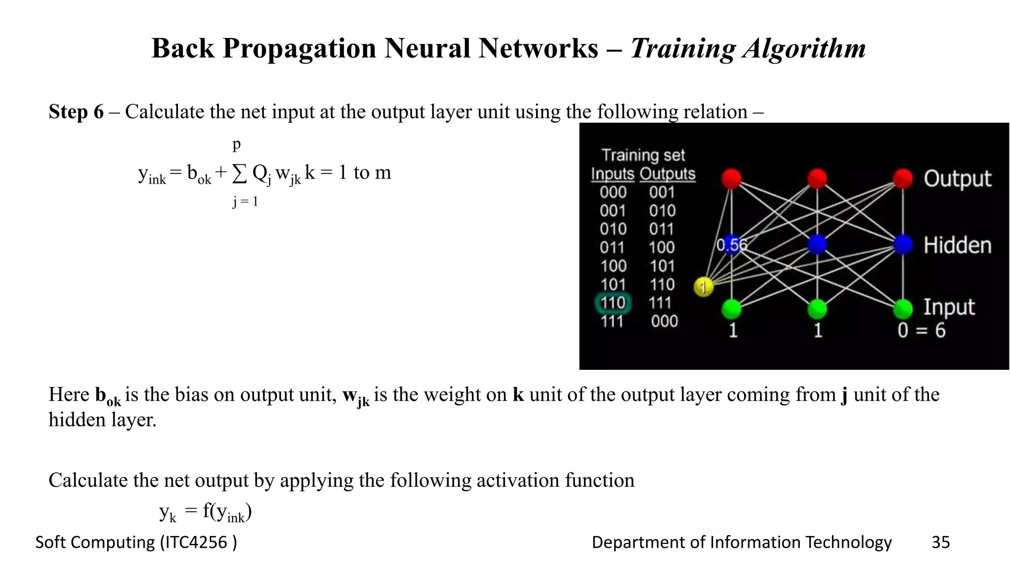
Step 6 – Calculate the net input at the output layer unit using the following relation –
p
yink = bok + ∑ Qj wjk k = 1 to m
j = 1
Here bok is the bias on output unit, wjk is the weight on k unit of the output layer coming from j unit of the
hidden layer.
Calculate the net output by applying the following activation function
yk = f(yink)
Department of Information Technology 36Soft Computing (ITC4256 )
Back Propagation Neural Networks – Training
Algorithm
Phase 2
Step 7 − Compute the error correcting term, in correspondence with the target
pattern received at each output unit, as follows −
δk = (tk−yk) f′ (yink)
On this basis, update the weight and bias as follows −
Δvjk=αδkQij
Δb0k=αδk
Then, send δk back to the hidden layer.
Department of Information Technology 37Soft Computing (ITC4256 )
Back Propagation Neural Networks – Training Algorithm
Step 8 − Now each hidden unit will be the sum of its delta inputs from the
output units.
m
δinj = ∑ δkwjk
k=1
Error term can be calculated as follows −
δj=δinjf′(Qinj)
On this basis, update the weight and bias as follows −
Δwij=αδjxi
Δb0j=αδj
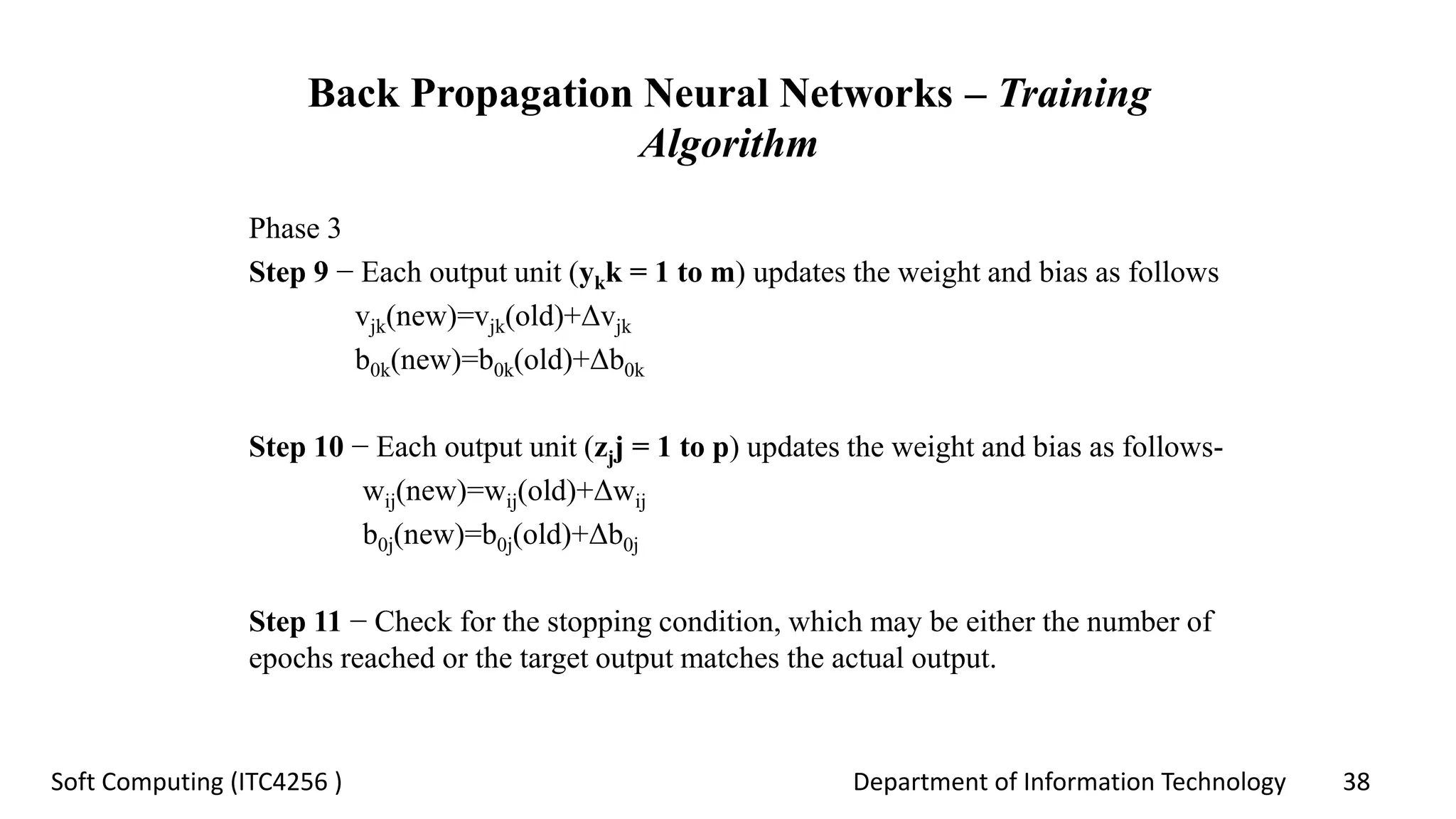
Department of Information Technology 38Soft Computing (ITC4256 )
Back Propagation Neural Networks – Training
Algorithm
Phase 3
Step 9 − Each output unit (ykk = 1 to m) updates the weight and bias as follows
vjk(new)=vjk(old)+Δvjk
b0k(new)=b0k(old)+Δb0k
Step 10 − Each output unit (zjj = 1 to p) updates the weight and bias as follows-
wij(new)=wij(old)+Δwij
b0j(new)=b0j(old)+Δb0j
Step 11 − Check for the stopping condition, which may be either the number of
epochs reached or the target output matches the actual output.
Department of Information Technology 39Soft Computing (ITC4256 )
Generalized Delta Learning Rule
• Delta rule works only for the output layer.
• On the other hand, generalized delta rule, also called as back-propagation rule, is a
way of creating the desired values of the hidden layer.
Mathematical Formulation
For the activation function yk=f(yink) the derivation of net input on Hidden layer as well
as on output layer can be given by
yink=∑ ziwjk
i
And yinj=∑ xivij
i
Now the error which has to be minimized is
E=1/2 ∑ [tk−yk]2
k
Department of Information Technology 40Soft Computing (ITC4256 )
Generalized Delta Learning Rule (Cont…)
By using the chain rule, we have
∂E / ∂wjk = ∂ / ∂wjk(1 / 2 ∑ [tk−yk]2)
k
= ∂ / ∂wjk ⟮1 / 2 [tk− t(yink)]2⟯
= −[tk − yk] ∂ / ∂wjk f(yink)
= −[tk−yk] f(yink) ∂ / ∂wjk(yink)
= −[tk−yk] f′(yink)zj
Now let us say δk = −[tk−yk] f′(yink)
The weights on connections to the hidden unit zj can be
given by −
∂E / ∂vij = −∑ δk ∂ / ∂vij(yink)
k
Department of Information Technology 41Soft Computing (ITC4256 )
Generalized Delta Learning Rule (Cont…)
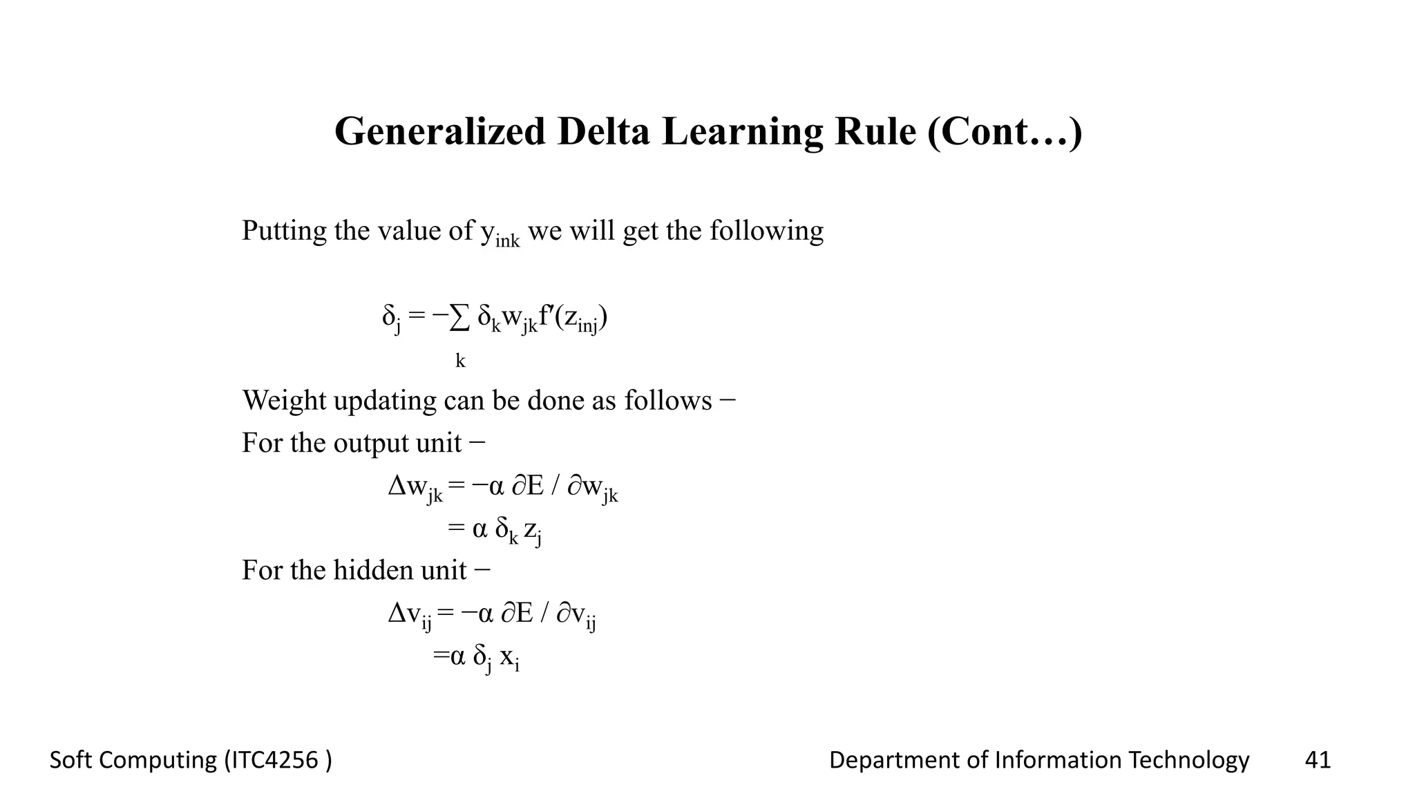
Putting the value of yink we will get the following
δj = −∑ δkwjkf′(zinj)
k
Weight updating can be done as follows −
For the output unit −
Δwjk = −α ∂E / ∂wjk
= α δk zj
For the hidden unit −
Δvij = −α ∂E / ∂vij
=α δj xi
Department of Information Technology 42Soft Computing (ITC4256 )
Quiz - Questions
1. Back Propagation Neural BPN is a multilayer neural network consisting of the
input layer, at least one ----------- layer and output layer.
2. The hidden layer as well as the output layer also has bias, whose weight is
always 2, on them.
a) true b) false
3. What parameters has to be initialized to start the training?
4. For easy calculation and simplicity, take -------- values.
a) 2 b) 3 c) random d) none
5. Delta rule works only for the -------- layer.
Department of Information Technology 43Soft Computing (ITC4256 )
Quiz - Answers
1. Back Propagation Neural BPN is a multilayer neural network consisting of the
input layer, at least one ----------- layer and output layer.
hidden
2. The hidden layer as well as the output layer also has bias, whose weight is
always 2, on them.
b) false
3. What parameters has to be initialized to start the training?
i. Weights ii. Learning rate α
4. For easy calculation and simplicity, take -------- values.
c) random
5. Delta rule works only for the --------- layer.
output
Department of Information Technology 44Soft Computing (ITC4256 )
Action Plan
• Supervised Learning Network (Cont…)
- Introduction to LVQ
- LVQ architecture
- LVQ training algorithm
- LVQ variants
- Introduction to TDNN
- Implementation of TDNN
- Building & using TDNN
• Quiz at the end of session
Department of Information Technology 45Soft Computing (ITC4256 )
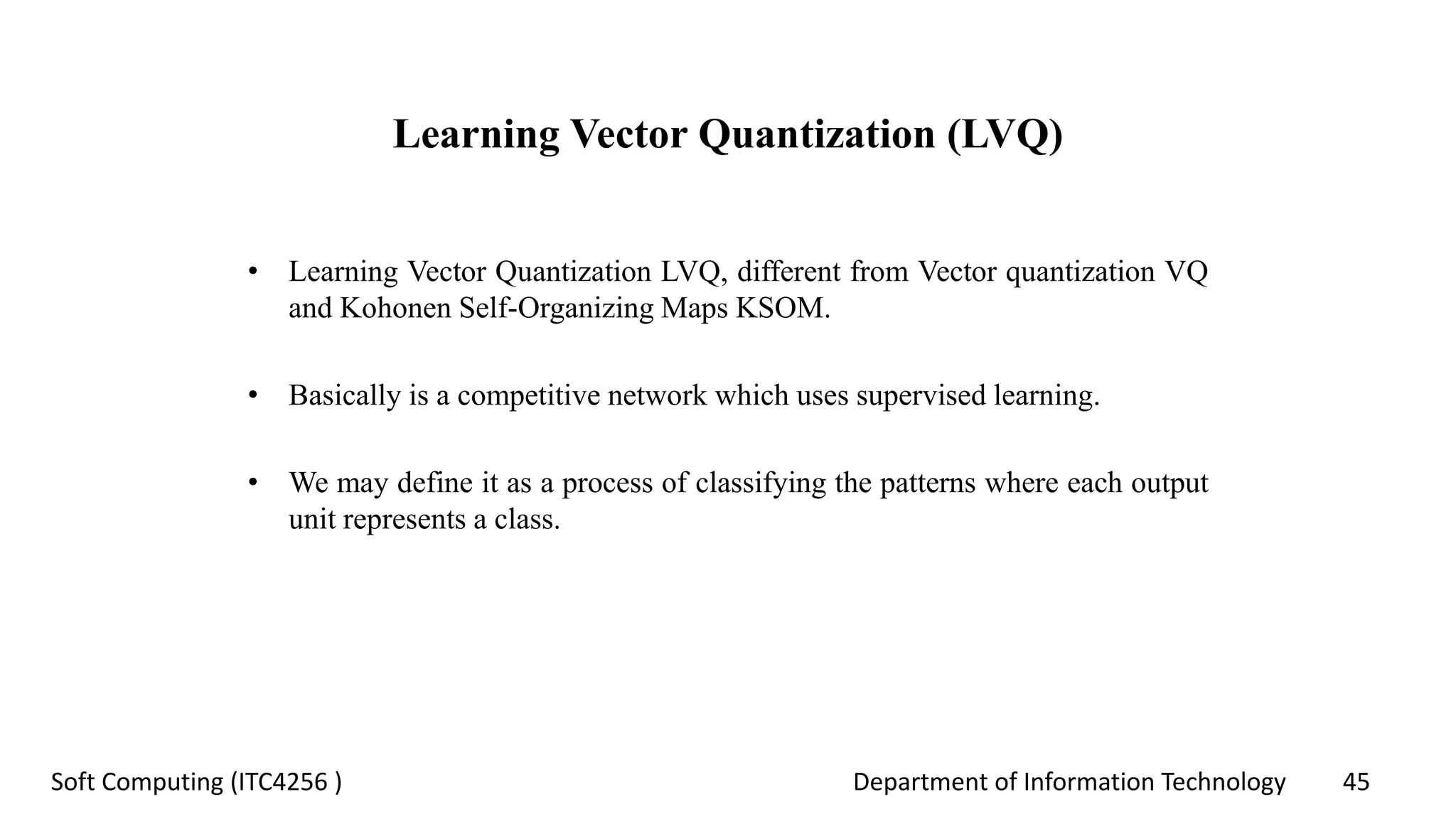
Learning Vector Quantization (LVQ)
• Learning Vector Quantization LVQ, different from Vector quantization VQ
and Kohonen Self-Organizing Maps KSOM.
• Basically is a competitive network which uses supervised learning.
• We may define it as a process of classifying the patterns where each output
unit represents a class.
Department of Information Technology 46Soft Computing (ITC4256 )
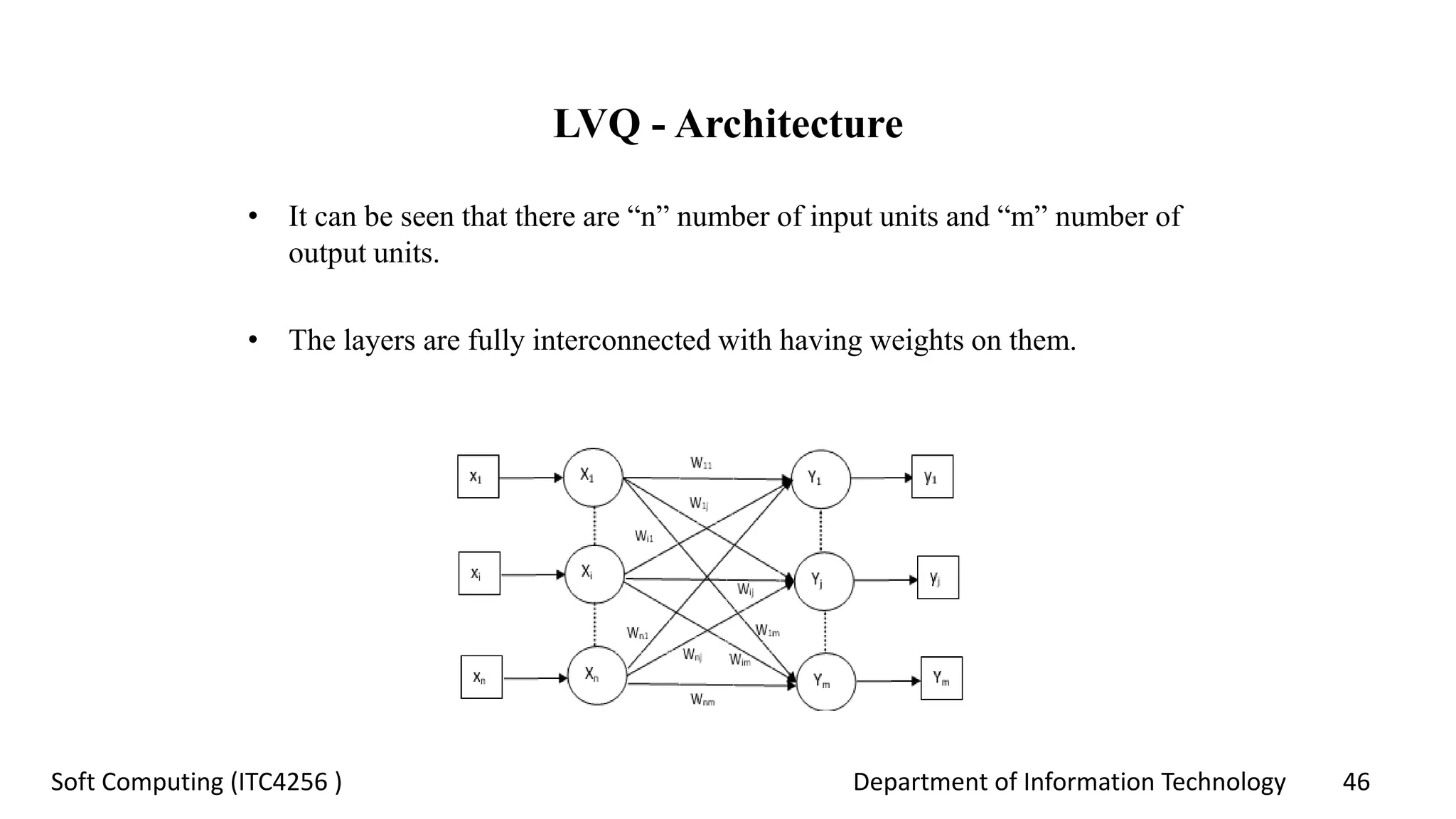
LVQ - Architecture
• It can be seen that there are “n” number of input units and “m” number of
output units.
• The layers are fully interconnected with having weights on them.
Department of Information Technology 47Soft Computing (ITC4256 )
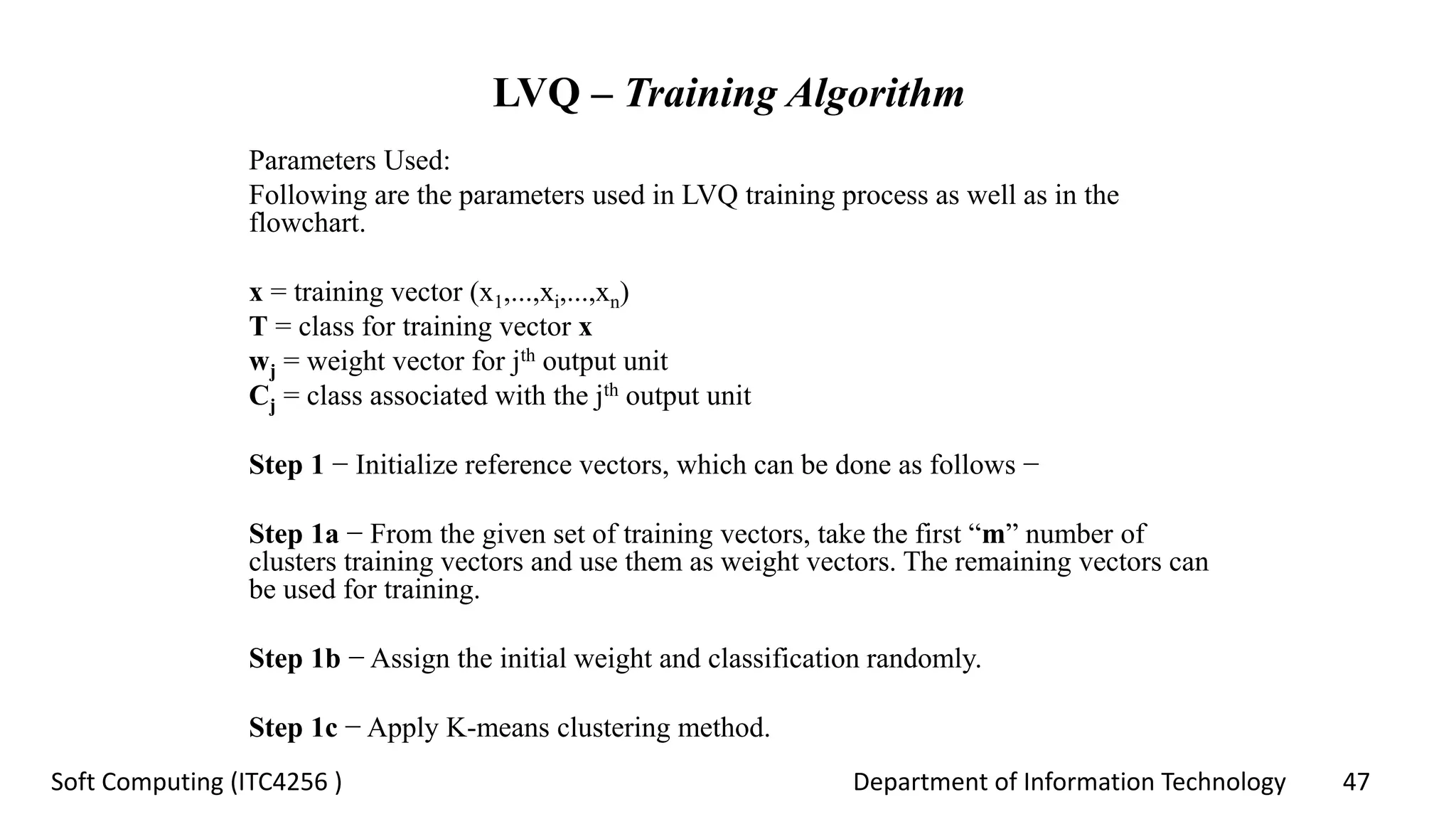
LVQ – Training Algorithm
Parameters Used:
Following are the parameters used in LVQ training process as well as in the
flowchart.
x = training vector (x1,...,xi,...,xn)
T = class for training vector x
wj = weight vector for jth output unit
Cj = class associated with the jth output unit
Step 1 − Initialize reference vectors, which can be done as follows −
Step 1a − From the given set of training vectors, take the first “m” number of
clusters training vectors and use them as weight vectors. The remaining vectors can
be used for training.
Step 1b − Assign the initial weight and classification randomly.
Step 1c − Apply K-means clustering method.
Department of Information Technology 48Soft Computing (ITC4256 )
LVQ – Training Algorithm (Cont…)
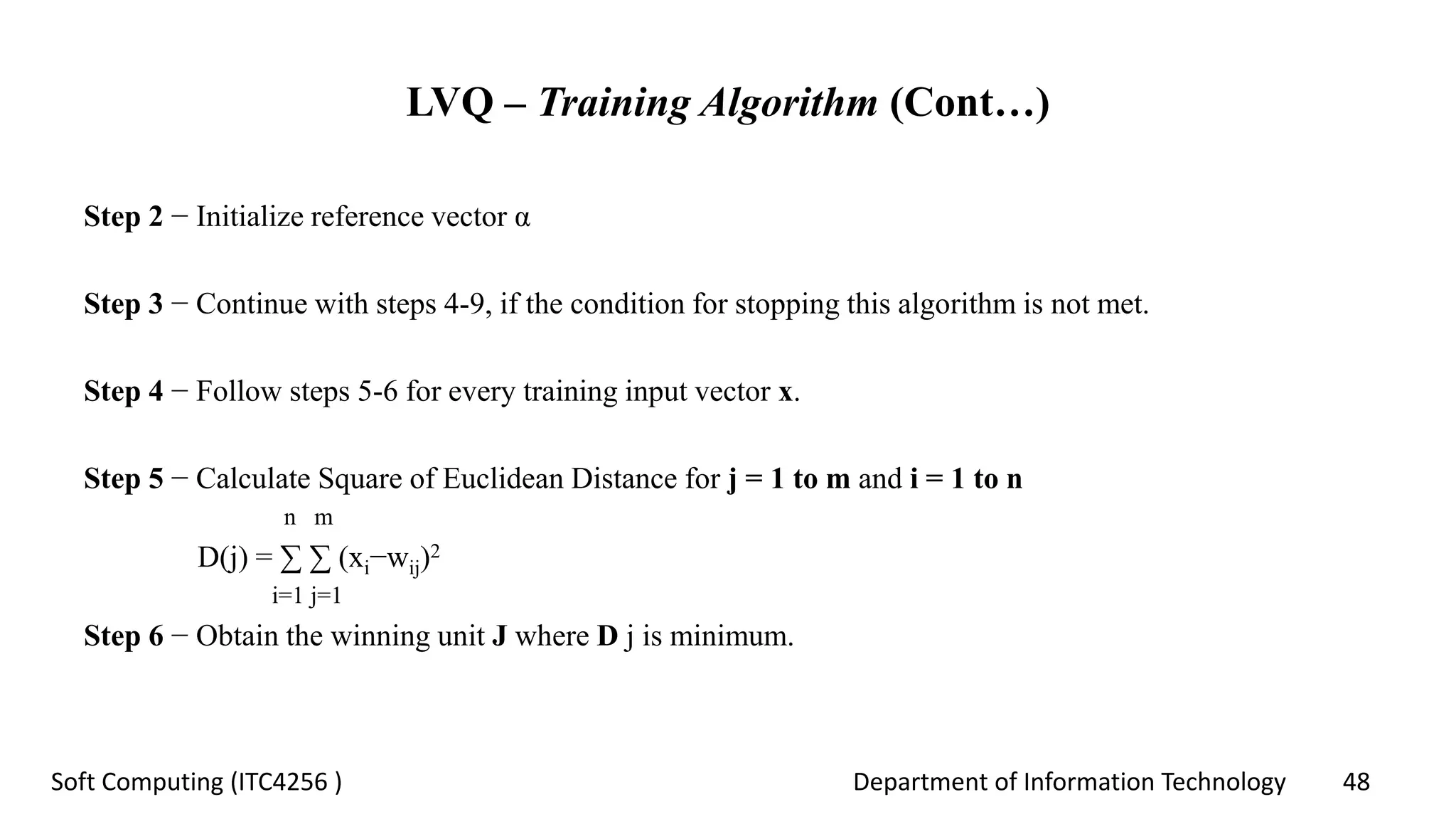
Step 2 − Initialize reference vector α
Step 3 − Continue with steps 4-9, if the condition for stopping this algorithm is not met.
Step 4 − Follow steps 5-6 for every training input vector x.
Step 5 − Calculate Square of Euclidean Distance for j = 1 to m and i = 1 to n
n m
D(j) = ∑ ∑ (xi−wij)2
i=1 j=1
Step 6 − Obtain the winning unit J where D j is minimum.
Department of Information Technology 49Soft Computing (ITC4256 )
LVQ – Training Algorithm (Cont…)
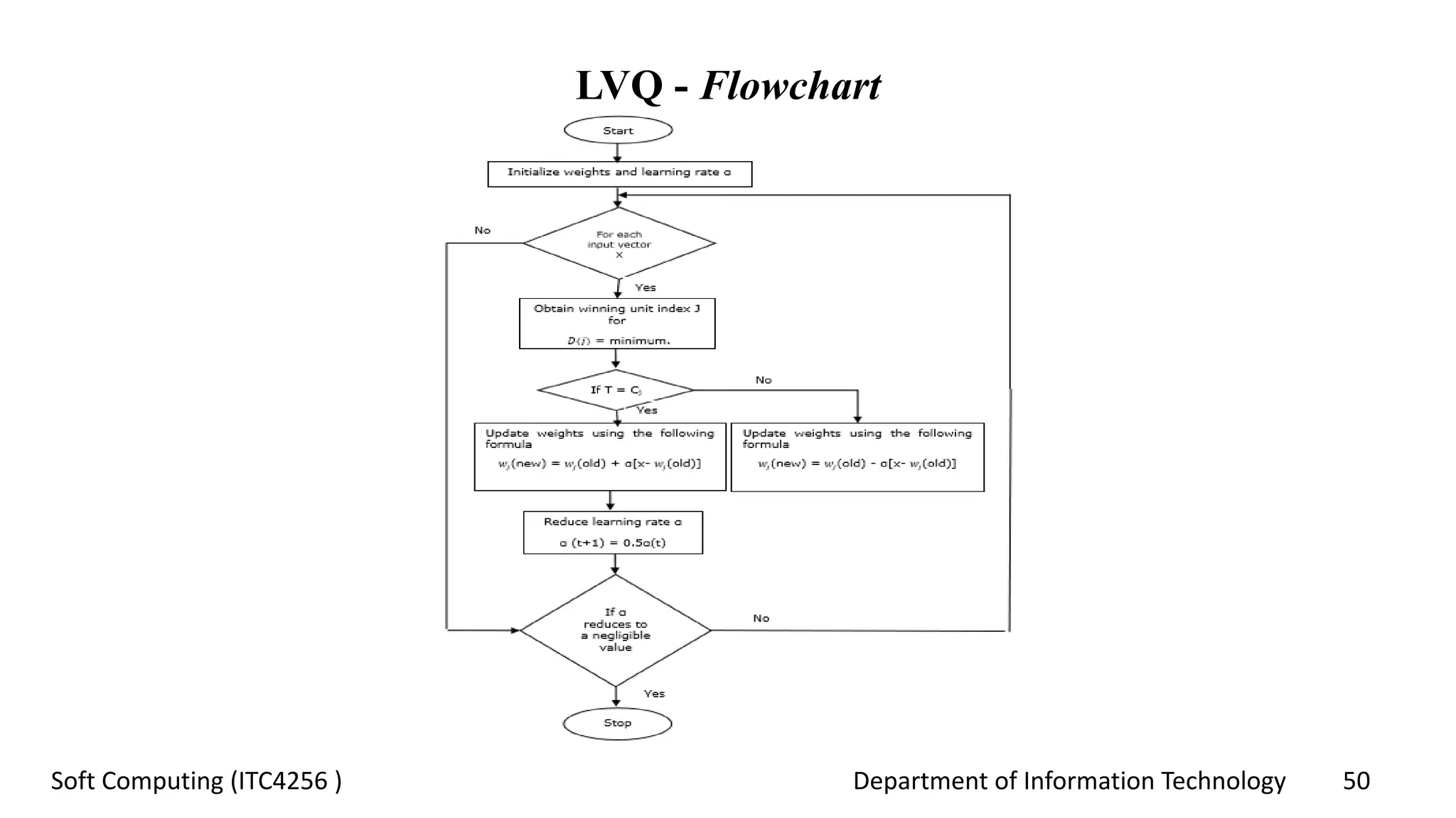
Step 7 − Calculate the new weight of the winning unit by the following relation −
if T = Cj then wj(new) = wj(old) + α[x−wj(old)]
if T ≠ Cj then wj(new) = wj(old) − α[x−wj(old)]
Step 8 − Reduce the learning rate α.
Step 9 − Test for the stopping condition. It may be as follows −
• Maximum number of epochs reached.
• Learning rate reduced to a negligible value.
Department of Information Technology 50Soft Computing (ITC4256 )
LVQ - Flowchart
Department of Information Technology 51Soft Computing (ITC4256 )
LVQ - Variants
• Three other variants namely LVQ2, LVQ2.1 and LVQ3 have been
developed by Kohonen.
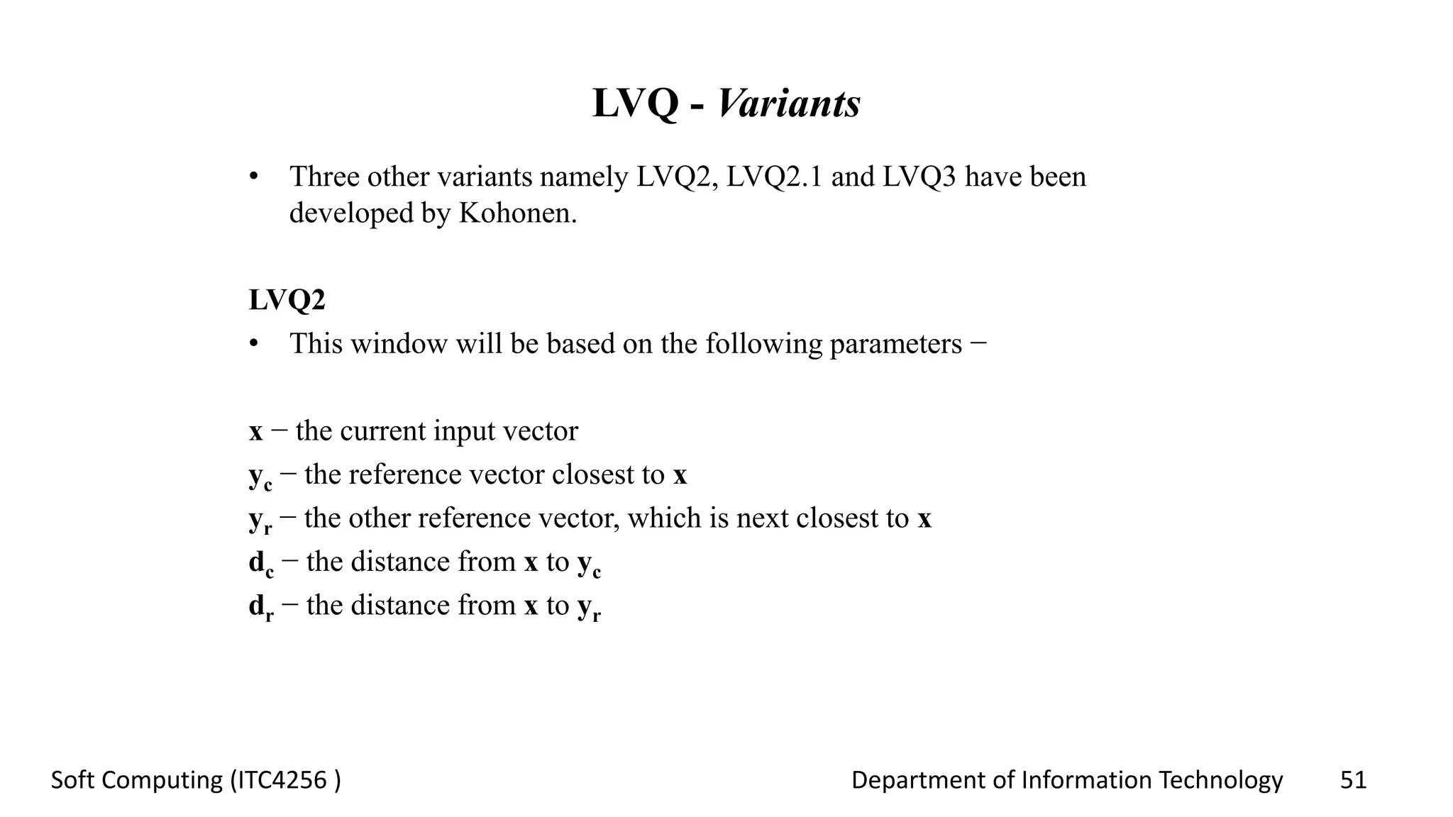
LVQ2
• This window will be based on the following parameters −
x − the current input vector
yc − the reference vector closest to x
yr − the other reference vector, which is next closest to x
dc − the distance from x to yc
dr − the distance from x to yr
Department of Information Technology 52Soft Computing (ITC4256 )
LVQ - Variants
• The input vector x falls in the window, if
dc / dr > 1 − θ and dr / dc > 1 + θ
• Here, θ is the number of training samples.
• Updating can be done with the following formula −
yc (t+1) = yc(t) + α(t)[x(t) − yc(t)] belongs to different class
yr (t+1) = yr(t) + α(t)[x(t) − yr(t)] belongs to same class
• Here α is the learning rate.
Department of Information Technology 53Soft Computing (ITC4256 )
LVQ - Variants
LVQ2.1
• In LVQ2.1, we will take the two closest vectors namely yc1 and yc2 and
the condition for window is as follows −
Min [ dc1 / dc2, dc2 / dc1] > (1−θ)
Max [ dc1 / dc2, dc2 / dc1] < (1+θ)
• Updating can be done with the following formula −
yc1(t+1) = yc1(t) + α(t) [x(t) − yc1(t)] belongs to different class
yc2(t+1) = yc2(t) + α(t) [x(t) − yc2(t)] belongs to same class
• Here, α is the learning rate.
Department of Information Technology 54Soft Computing (ITC4256 )
LVQ - Variants
LVQ3
• In LVQ3, we will take the two closest vectors namely yc1 and yc2 and the
condition for window is as follows −
Min [ dc1 / dc2, dc2 / dc1] > (1 − θ) (1 + θ)
• Here θ ≈ 0.2
• Updating can be done with the following formula −
yc1(t+1) = yc1(t) + β(t) [x(t) − yc1(t)] belongs to different class
yc2(t+1) = yc2(t) + β(t) [x(t) − yc2(t)] belongs to same class
• Here β is the multiple of the learning rate α and β=mα(t) for every
0.1 < m < 0.5
Department of Information Technology 55Soft Computing (ITC4256 )
Time Delay Neural Network (TDNN)
• Time delay networks, introduced by Alex Waibel, are a group of neural networks that have a special
topology.
• They are used for position independent recognition of features within a larger pattern.
Department of Information Technology 56Soft Computing (ITC4256 )
TDNNs (Cont…)
• Feature: A component of the pattern to be learned.
• Feature Unit: The unit connected with the feature to be learned.
• Delay: In order to be able to recognize patterns place or time-invariant,
older activation and connection values of the feature units have to be
stored.
Department of Information Technology 57Soft Computing (ITC4256 )
TDNNs (Cont…)
• Receptive Field: The feature units and their delays are fully connected to
the original units of the subsequent layer.
• Total Delay Length: The length of the layer.
• Coupled Links: Each link in a receptive field is reduplicated for every
subsequent step of time up to the total delay length.
Department of Information Technology 58Soft Computing (ITC4256 )
TDNN Implementation in SNNS
• The original time delay algorithm was slightly modified for implementation
in Stuttgart Neural Network Simulator (SNNS), since it requires either
variable network sizes or fixed length input patterns.
• The coupled links are implemented as one physical (i.e. normal) link and a
set of logical links associated with it.
Department of Information Technology 59Soft Computing (ITC4256 )
Building and Using a Time Delay Network
• In SNNS, TDNNs should be generated only with the tool BIGNET (Time
Delay).
• After the creation of the net, the unit activation function Act_TD_Logistic,
the update function TimeDelay_Order, and the learning function
TimeDelayBackprop have to be assigned in the usual way.
• If the application requires variable pattern length, a tool to segment these
patterns into fitting pieces has to be applied.
Department of Information Technology 60Soft Computing (ITC4256 )
Quiz - Questions
1. Each output unit represents a ----------.
a) class b) object c) data d) none
2. In step 1b of LVQ training algorithm, assign the initial weight and
------------- randomly.
3. Three other variants namely LVQ2, LVQ2.1 and LVQ3 have been
developed by ------------.
4. The coupled links are implemented as one physical link and a
set of logical links associated with it.
a) true b) false
5. In SNNS, TDNNs should be generated only with the tool -----------.
Department of Information Technology 61Soft Computing (ITC4256 )
Quiz - Answers
1. Each output unit represents a ----------.
a) class
2. In step 1b of LVQ training algorithm, assign the initial weight and
------------- randomly.
classification
3. Three other variants namely LVQ2, LVQ2.1 and LVQ3 have been
developed by ------------ .
Kohonen
4. The coupled links are implemented as one physical link and a
set of logical links associated with it.
a) true
5. In SNNS, TDNNs should be generated only with the tool ----------- .
BIGNET

Supervised learning network

  • 1.
    Department of InformationTechnology 1Soft Computing (ITC4256 ) Supervised learning network Dr. C.V. Suresh Babu Professor Department of IT Hindustan Institute of Science & Technology
  • 2.
    Department of InformationTechnology 2Soft Computing (ITC4256 ) Discussion Topics • Supervised Learning Networks - Perceptron networks - Perceptron network- training algorithm • Quiz at the end of session.
  • 3.
    Department of InformationTechnology 3Soft Computing (ITC4256 ) Introduction
  • 4.
    Department of InformationTechnology 4Soft Computing (ITC4256 ) Perceptron Networks • Developed by Frank Rosenblatt by using McCulloch and Pitts model, perceptron is the basic operational unit of artificial neural networks.
  • 5.
    Department of InformationTechnology 5Soft Computing (ITC4256 ) Perceptron Networks (Cont…) • Perceptron thus has the following three basic elements: - Links - Adder - Activation function • Perceptron network can be trained for single output unit as well as multiple output units.
  • 6.
    Department of InformationTechnology 6Soft Computing (ITC4256 )
  • 7.
    Department of InformationTechnology 7Soft Computing (ITC4256 ) Perceptron Networks – Training Algorithm Training Algorithm for Single Output Unit: Step 1 − Initialize the following to start the training − • Weights • Bias • Learning rate α For easy calculation and simplicity, weights and bias must be set equal to 0 and the learning rate must be set equal to 1. Step 2 − Continue step 3-8 when the stopping condition is not true. Step 3 − Continue step 4-6 for every training vector x. Step 4 − Activate each input unit as follows − xi=si(i=1 to n)
  • 8.
    Department of InformationTechnology 8Soft Computing (ITC4256 ) Perceptron Networks – Training Algorithm (Cont…) Step 5 − Now obtain the net input with the following relation − n yin = b + ∑ xi.wi i Here ‘b’ is bias and ‘n’ is the total number of input neurons. Step 6 − Apply the following activation function to obtain the final output. 1 if yin > θ f( yin ) = 0 if -θ < yin < θ -1 if yin < -θ
  • 9.
    Department of InformationTechnology 9Soft Computing (ITC4256 ) Perceptron Networks – Training Algorithm (Cont…) Step 7 − Adjust the weight and bias as follows − Case 1 − if y ≠ t then, wi(new)=wi(old)+α txi b(new)=b(old)+αt Case 2 − if y = t then, wi(new)=wi(old) b(new)=b(old) Here ‘y’ is the actual output and ‘t’ is the desired/target output. Step 8 − Test for the stopping condition, which would happen when there is no change in weight.
  • 10.
    Department of InformationTechnology 10Soft Computing (ITC4256 ) Perceptron Networks – Training Algorithm (Cont…) Training Algorithm for Multiple Output Units: Architecture of perceptron for multiple output classes.
  • 11.
    Department of InformationTechnology 11Soft Computing (ITC4256 ) Perceptron Networks – Training Algorithm (Cont…) Step 1 − Initialize the following to start the training − • Weights • Bias • Learning rate α For easy calculation and simplicity, weights and bias must be set equal to 0 and the learning rate must be set equal to 1. Step 2 − Continue step 3-8 when the stopping condition is not true. Step 3 − Continue step 4-6 for every training vector x. Step 4 − Activate each input unit as follows − xi=si(i=1 to n)
  • 12.
    Department of InformationTechnology 12Soft Computing (ITC4256 ) Perceptron Networks – Training Algorithm (Cont…) Step 5 − Now obtain the net input with the following relation − n yin = b + ∑ xi.wij i Here ‘b’ is bias and ‘n’ is the total number of input neurons. Step 6 − Apply the following activation function to obtain the final output for each output unit j=1 to m, 1 if yin > θ f( yin ) = 0 if -θ < yin < θ -1 if yin < -θ
  • 13.
    Department of InformationTechnology 13Soft Computing (ITC4256 ) Perceptron Networks – Training Algorithm (Cont…) Step 7 − Adjust the weight and bias for x = 1 to n and j = 1 to m as follows − Case 1 − if yj ≠ tj then, wij(new) = wij(old) + α tjxi bj(new) = bj(old) + α tj Case 2 − if yj = tj then, wij(new) = wij(old) bj(new) = bj(old) Here ‘y’ is the actual output and ‘t’ is the desired/target output. Step 8 − Test for the stopping condition, which will happen when there is no change in weight.
  • 14.
    Department of InformationTechnology 14Soft Computing (ITC4256 ) Quiz - Questions 1. What are the 3 basic elements of perceptron? 2. ---------- is the basic operational unit of artificial neural networks. 3. Perceptron network can be trained only for single output unit. a) true b) false 4. What are the parameters to be initialized to start the training? 5. What will happen when there is no change in weight?
  • 15.
    Department of InformationTechnology 15Soft Computing (ITC4256 ) Quiz - Answers 1. What are the 3 basic elements of perceptron? i. links ii. adder iii. activation function 2. ---------- is the basic operational unit of artificial neural networks. Perceptron 3. Perceptron network can be trained only for single output unit. b) false 4. Weights, bias and learning rate α 5. Stopping condition
  • 16.
    Department of InformationTechnology 16Soft Computing (ITC4256 ) Action Plan • Supervised Learning Networks (Cont…) - Introduction to adaptive linear neuron - Adaptive linear neuron architecture - Adaptive linear neuron training algorithm - Introduction to multiple adaptive linear neuron - Multiple adaptive linear neuron architecture - Multiple adaptive linear neuron training algorithm • Quiz at the end of session.
  • 17.
    Department of InformationTechnology 17Soft Computing (ITC4256 ) Adaptive Linear Neuron • Adaline which stands for Adaptive Linear Neuron, is a network having a single linear unit. • It was developed by Widrow and Hoff in 1960.
  • 18.
    Department of InformationTechnology 18Soft Computing (ITC4256 ) Adaptive Linear Neuron - Architecture • The basic structure of Adaline is similar to perceptron having an extra feedback loop with the help of which the actual output is compared with the desired/target output. • After comparison on the basis of training algorithm, the weights and bias will be updated.
  • 19.
    Department of InformationTechnology 19Soft Computing (ITC4256 ) Adaptive Linear Neuron – Training Algorithm Step 1 − Initialize the following to start the training − • Weights • Bias • Learning rate α For easy calculation and simplicity, weights and bias must be set equal to 0 and the learning rate must be set equal to 1. Step 2 − Continue step 3-8 when the stopping condition is not true. Step 3 − Continue step 4-6 for every bipolar training pair s:t. Step 4 − Activate each input unit as follows: xi=si(i = 1 to n)
  • 20.
    Department of InformationTechnology 20Soft Computing (ITC4256 ) Adaptive Linear Neuron – Training Algorithm Step 5 − Obtain the net input with the following relation − n yin = b + ∑ xi.wi i Here ‘b’ is bias and ‘n’ is the total number of input neurons. Step 6 − Apply the following activation function to obtain the final output. 1 if yin > 0 f( yin ) = -1 if yin < 0
  • 21.
    Department of InformationTechnology 21Soft Computing (ITC4256 ) Adaptive Linear Neuron – Training Algorithm Step 7 − Adjust the weight and bias as follows − Case 1 − if y ≠ t then, wi(new) = wi(old) + α(t – yin) xi b(new) = b(old) + α(t – yin) Case 2 − if y = t then, wi(new) = wi(old) b(new) = b(old) Here ‘y’ is the actual output and ‘t’ is the desired/target output. (t – yin) is the computed error. Step 8 − Test for the stopping condition, which would happen when there is no change in weight or the highest weight change occurred during training is smaller than the specified tolerance.
  • 22.
    Department of InformationTechnology 22Soft Computing (ITC4256 ) Multiple Adaptive Linear Neuron • Madaline which stands for Multiple Adaptive Linear Neuron, is a network which consists of many Adalines in parallel. • It will have a single output unit.
  • 23.
    Department of InformationTechnology 23Soft Computing (ITC4256 ) Multiple Adaptive Linear Neuron - Architecture • The architecture of Madaline consists of “n” neurons of the input layer, “m” neurons of the Adaline layer, and 1 neuron of the Madaline layer. • The Adaline layer can be considered as the hidden layer as it is between the input layer and the output layer, i.e. the Madaline layer.
  • 24.
    Department of InformationTechnology 24Soft Computing (ITC4256 ) Multiple Adaptive Linear Neuron – Training Algorithm Step 1 − Initialize the following to start the training − • Weights • Bias • Learning rate α For easy calculation and simplicity, weights and bias must be set equal to 0 and the learning rate must be set equal to 1. Step 2 − Continue step 3-8 when the stopping condition is not true. Step 3 − Continue step 4-6 for every bipolar training pair s:t. Step 4 − Activate each input unit as follows: xi=si(i = 1 to n)
  • 25.
    Department of InformationTechnology 25Soft Computing (ITC4256 ) Multiple Adaptive Linear Neuron – Training Algorithm Step 5 − Obtain the net input at each hidden layer, i.e. the Adaline layer with the following relation − n Qinj = bj + ∑ xi.wij j = 1 to m i Here ‘b’ is bias and ‘n’ is the total number of input neurons. Step 6 − Apply the following activation function to obtain the final output at the Adaline and the Madaline layer - 1 if x > 0 f(x) = -1 if x < 0 Output at the hidden Adaline unit: Qj = f ( Qinj ) m Final output of the network: y = f ( yin ) i.e. yinj = b0 + ∑ Qj vj j=1
  • 26.
    Department of InformationTechnology 26Soft Computing (ITC4256 ) Multiple Adaptive Linear Neuron – Training Algorithm
  • 27.
    Department of InformationTechnology 27Soft Computing (ITC4256 ) Multiple Adaptive Linear Neuron – Training Algorithm Step 7 − Calculate the error and adjust the weights as follows − Case 1 − if y ≠ t and t = 1 then, wij(new) = wij(old) + α(1 – Qinj) xi bj(new) = bj(old) + α(1 – Qinj) In this case, the weights would be updated on Qj where the net input is close to 0 because t = 1. Case 2 − if y ≠ t and t = -1 then, wik(new) = wik(old) + α(-1 – Qink) xi bk(new) = bk(old) + α(-1 – Qink) In this case, the weights would be updated on Qk where the net input is positive because t = -1. Here ‘y’ is the actual output and ‘t’ is the desired/target output. Case 3 – if y = t then, there would be no change in weights. Step 8 − Test for the stopping condition.
  • 28.
    Department of InformationTechnology 28Soft Computing (ITC4256 ) Quiz - Questions 1. Adaline which stands for Adaptive Linear Neuron, is a network having a -------- linear unit. a) triple b) double c) single d) multiple 2. Madaline which stands for Multiple Adaptive Linear Neuron, is a network which consists of many ---------- in parallel. a) adalines b) neurons c) ports d) none 3. Madaline has a --------- output unit. 4. The weights and the --------- are adjustable. 5. For easy calculation and simplicity, weights and bias must be set equal to 1 and the learning rate must be set equal to 0. a) true b) false
  • 29.
    Department of InformationTechnology 29Soft Computing (ITC4256 ) Quiz - Answers 1. Adaline which stands for Adaptive Linear Neuron, is a network having a -------- linear unit. c) single 2. Madaline which stands for Multiple Adaptive Linear Neuron, is a network which consists of many ---------- in parallel. a) adalines 3. Madaline has a --------- output unit. single 4. The weights and the --------- are adjustable. bias 5. For easy calculation and simplicity, weights and bias must be set equal to 1 and the learning rate must be set equal to 0. b) false
  • 30.
    Department of InformationTechnology 30Soft Computing (ITC4256 ) Action Plan • Supervised Learning Networks (Cont…) - Introduction to back propagation neural networks - Back propagation network architecture - Back propagation network training algorithm - Generalized delta learning rule • Quiz at the end of session
  • 31.
    • Back PropagationNeural BPN is a multilayer neural network consisting of the input layer, at least one hidden layer and output layer. • As its name suggests, back propagating will take place in this network. – The error which is calculated at the output layer, by comparing the target output and the actual output, will be propagated back towards the input layer.
  • 32.
    Department of InformationTechnology 32Soft Computing (ITC4256 ) Back Propagation Neural Networks - Architecture • As shown in the diagram, the architecture of BPN has three interconnected layers having weights on them. • The hidden layer as well as the output layer also has bias, whose weight is always 1, on them.
  • 33.
    Department of InformationTechnology 33Soft Computing (ITC4256 ) Back Propagation Neural Networks – Training Algorithm For training, BPN will use binary sigmoid activation function. The training of BPN will have the following three phases. - Phase 1: Feed Forward Phase - Phase 2: Back Propagation of error - Phase 3: Updating of weights All these steps will be concluded in the algorithm as follows Step 1 − Initialize the following to start the training − - Weights - Learning rate α For easy calculation and simplicity, take some small random values. Step 2 − Continue step 3-11 when the stopping condition is not true. Step 3 − Continue step 4-10 for every training pair.
  • 34.
    Department of InformationTechnology 34Soft Computing (ITC4256 ) Back Propagation Neural Networks – Training Algorithm Phase 1 Step 4 − Each input unit receives input signal xi and sends it to the hidden unit for all i = 1 to n Step 5 − Calculate the net input at the hidden unit using the following relation- n Qinj = b0j + ∑ xi vij j = 1 to p i=1 Here boj is the bias on hidden unit, vij is the weight on j unit of the hidden layer coming from i unit of the input layer. Now calculate the net output by applying the following activation function Qj = f(Qinj) Send these output signals of the hidden layer units to the output layer units.
  • 35.
    Department of InformationTechnology 35Soft Computing (ITC4256 ) Back Propagation Neural Networks – Training Algorithm Step 6 – Calculate the net input at the output layer unit using the following relation – p yink = bok + ∑ Qj wjk k = 1 to m j = 1 Here bok is the bias on output unit, wjk is the weight on k unit of the output layer coming from j unit of the hidden layer. Calculate the net output by applying the following activation function yk = f(yink)
  • 36.
    Department of InformationTechnology 36Soft Computing (ITC4256 ) Back Propagation Neural Networks – Training Algorithm Phase 2 Step 7 − Compute the error correcting term, in correspondence with the target pattern received at each output unit, as follows − δk = (tk−yk) f′ (yink) On this basis, update the weight and bias as follows − Δvjk=αδkQij Δb0k=αδk Then, send δk back to the hidden layer.
  • 37.
    Department of InformationTechnology 37Soft Computing (ITC4256 ) Back Propagation Neural Networks – Training Algorithm Step 8 − Now each hidden unit will be the sum of its delta inputs from the output units. m δinj = ∑ δkwjk k=1 Error term can be calculated as follows − δj=δinjf′(Qinj) On this basis, update the weight and bias as follows − Δwij=αδjxi Δb0j=αδj
  • 38.
    Department of InformationTechnology 38Soft Computing (ITC4256 ) Back Propagation Neural Networks – Training Algorithm Phase 3 Step 9 − Each output unit (ykk = 1 to m) updates the weight and bias as follows vjk(new)=vjk(old)+Δvjk b0k(new)=b0k(old)+Δb0k Step 10 − Each output unit (zjj = 1 to p) updates the weight and bias as follows- wij(new)=wij(old)+Δwij b0j(new)=b0j(old)+Δb0j Step 11 − Check for the stopping condition, which may be either the number of epochs reached or the target output matches the actual output.
  • 39.
    Department of InformationTechnology 39Soft Computing (ITC4256 ) Generalized Delta Learning Rule • Delta rule works only for the output layer. • On the other hand, generalized delta rule, also called as back-propagation rule, is a way of creating the desired values of the hidden layer. Mathematical Formulation For the activation function yk=f(yink) the derivation of net input on Hidden layer as well as on output layer can be given by yink=∑ ziwjk i And yinj=∑ xivij i Now the error which has to be minimized is E=1/2 ∑ [tk−yk]2 k
  • 40.
    Department of InformationTechnology 40Soft Computing (ITC4256 ) Generalized Delta Learning Rule (Cont…) By using the chain rule, we have ∂E / ∂wjk = ∂ / ∂wjk(1 / 2 ∑ [tk−yk]2) k = ∂ / ∂wjk ⟮1 / 2 [tk− t(yink)]2⟯ = −[tk − yk] ∂ / ∂wjk f(yink) = −[tk−yk] f(yink) ∂ / ∂wjk(yink) = −[tk−yk] f′(yink)zj Now let us say δk = −[tk−yk] f′(yink) The weights on connections to the hidden unit zj can be given by − ∂E / ∂vij = −∑ δk ∂ / ∂vij(yink) k
  • 41.
    Department of InformationTechnology 41Soft Computing (ITC4256 ) Generalized Delta Learning Rule (Cont…) Putting the value of yink we will get the following δj = −∑ δkwjkf′(zinj) k Weight updating can be done as follows − For the output unit − Δwjk = −α ∂E / ∂wjk = α δk zj For the hidden unit − Δvij = −α ∂E / ∂vij =α δj xi
  • 42.
    Department of InformationTechnology 42Soft Computing (ITC4256 ) Quiz - Questions 1. Back Propagation Neural BPN is a multilayer neural network consisting of the input layer, at least one ----------- layer and output layer. 2. The hidden layer as well as the output layer also has bias, whose weight is always 2, on them. a) true b) false 3. What parameters has to be initialized to start the training? 4. For easy calculation and simplicity, take -------- values. a) 2 b) 3 c) random d) none 5. Delta rule works only for the -------- layer.
  • 43.
    Department of InformationTechnology 43Soft Computing (ITC4256 ) Quiz - Answers 1. Back Propagation Neural BPN is a multilayer neural network consisting of the input layer, at least one ----------- layer and output layer. hidden 2. The hidden layer as well as the output layer also has bias, whose weight is always 2, on them. b) false 3. What parameters has to be initialized to start the training? i. Weights ii. Learning rate α 4. For easy calculation and simplicity, take -------- values. c) random 5. Delta rule works only for the --------- layer. output
  • 44.
    Department of InformationTechnology 44Soft Computing (ITC4256 ) Action Plan • Supervised Learning Network (Cont…) - Introduction to LVQ - LVQ architecture - LVQ training algorithm - LVQ variants - Introduction to TDNN - Implementation of TDNN - Building & using TDNN • Quiz at the end of session
  • 45.
    Department of InformationTechnology 45Soft Computing (ITC4256 ) Learning Vector Quantization (LVQ) • Learning Vector Quantization LVQ, different from Vector quantization VQ and Kohonen Self-Organizing Maps KSOM. • Basically is a competitive network which uses supervised learning. • We may define it as a process of classifying the patterns where each output unit represents a class.
  • 46.
    Department of InformationTechnology 46Soft Computing (ITC4256 ) LVQ - Architecture • It can be seen that there are “n” number of input units and “m” number of output units. • The layers are fully interconnected with having weights on them.
  • 47.
    Department of InformationTechnology 47Soft Computing (ITC4256 ) LVQ – Training Algorithm Parameters Used: Following are the parameters used in LVQ training process as well as in the flowchart. x = training vector (x1,...,xi,...,xn) T = class for training vector x wj = weight vector for jth output unit Cj = class associated with the jth output unit Step 1 − Initialize reference vectors, which can be done as follows − Step 1a − From the given set of training vectors, take the first “m” number of clusters training vectors and use them as weight vectors. The remaining vectors can be used for training. Step 1b − Assign the initial weight and classification randomly. Step 1c − Apply K-means clustering method.
  • 48.
    Department of InformationTechnology 48Soft Computing (ITC4256 ) LVQ – Training Algorithm (Cont…) Step 2 − Initialize reference vector α Step 3 − Continue with steps 4-9, if the condition for stopping this algorithm is not met. Step 4 − Follow steps 5-6 for every training input vector x. Step 5 − Calculate Square of Euclidean Distance for j = 1 to m and i = 1 to n n m D(j) = ∑ ∑ (xi−wij)2 i=1 j=1 Step 6 − Obtain the winning unit J where D j is minimum.
  • 49.
    Department of InformationTechnology 49Soft Computing (ITC4256 ) LVQ – Training Algorithm (Cont…) Step 7 − Calculate the new weight of the winning unit by the following relation − if T = Cj then wj(new) = wj(old) + α[x−wj(old)] if T ≠ Cj then wj(new) = wj(old) − α[x−wj(old)] Step 8 − Reduce the learning rate α. Step 9 − Test for the stopping condition. It may be as follows − • Maximum number of epochs reached. • Learning rate reduced to a negligible value.
  • 50.
    Department of InformationTechnology 50Soft Computing (ITC4256 ) LVQ - Flowchart
  • 51.
    Department of InformationTechnology 51Soft Computing (ITC4256 ) LVQ - Variants • Three other variants namely LVQ2, LVQ2.1 and LVQ3 have been developed by Kohonen. LVQ2 • This window will be based on the following parameters − x − the current input vector yc − the reference vector closest to x yr − the other reference vector, which is next closest to x dc − the distance from x to yc dr − the distance from x to yr
  • 52.
    Department of InformationTechnology 52Soft Computing (ITC4256 ) LVQ - Variants • The input vector x falls in the window, if dc / dr > 1 − θ and dr / dc > 1 + θ • Here, θ is the number of training samples. • Updating can be done with the following formula − yc (t+1) = yc(t) + α(t)[x(t) − yc(t)] belongs to different class yr (t+1) = yr(t) + α(t)[x(t) − yr(t)] belongs to same class • Here α is the learning rate.
  • 53.
    Department of InformationTechnology 53Soft Computing (ITC4256 ) LVQ - Variants LVQ2.1 • In LVQ2.1, we will take the two closest vectors namely yc1 and yc2 and the condition for window is as follows − Min [ dc1 / dc2, dc2 / dc1] > (1−θ) Max [ dc1 / dc2, dc2 / dc1] < (1+θ) • Updating can be done with the following formula − yc1(t+1) = yc1(t) + α(t) [x(t) − yc1(t)] belongs to different class yc2(t+1) = yc2(t) + α(t) [x(t) − yc2(t)] belongs to same class • Here, α is the learning rate.
  • 54.
    Department of InformationTechnology 54Soft Computing (ITC4256 ) LVQ - Variants LVQ3 • In LVQ3, we will take the two closest vectors namely yc1 and yc2 and the condition for window is as follows − Min [ dc1 / dc2, dc2 / dc1] > (1 − θ) (1 + θ) • Here θ ≈ 0.2 • Updating can be done with the following formula − yc1(t+1) = yc1(t) + β(t) [x(t) − yc1(t)] belongs to different class yc2(t+1) = yc2(t) + β(t) [x(t) − yc2(t)] belongs to same class • Here β is the multiple of the learning rate α and β=mα(t) for every 0.1 < m < 0.5
  • 55.
    Department of InformationTechnology 55Soft Computing (ITC4256 ) Time Delay Neural Network (TDNN) • Time delay networks, introduced by Alex Waibel, are a group of neural networks that have a special topology. • They are used for position independent recognition of features within a larger pattern.
  • 56.
    Department of InformationTechnology 56Soft Computing (ITC4256 ) TDNNs (Cont…) • Feature: A component of the pattern to be learned. • Feature Unit: The unit connected with the feature to be learned. • Delay: In order to be able to recognize patterns place or time-invariant, older activation and connection values of the feature units have to be stored.
  • 57.
    Department of InformationTechnology 57Soft Computing (ITC4256 ) TDNNs (Cont…) • Receptive Field: The feature units and their delays are fully connected to the original units of the subsequent layer. • Total Delay Length: The length of the layer. • Coupled Links: Each link in a receptive field is reduplicated for every subsequent step of time up to the total delay length.
  • 58.
    Department of InformationTechnology 58Soft Computing (ITC4256 ) TDNN Implementation in SNNS • The original time delay algorithm was slightly modified for implementation in Stuttgart Neural Network Simulator (SNNS), since it requires either variable network sizes or fixed length input patterns. • The coupled links are implemented as one physical (i.e. normal) link and a set of logical links associated with it.
  • 59.
    Department of InformationTechnology 59Soft Computing (ITC4256 ) Building and Using a Time Delay Network • In SNNS, TDNNs should be generated only with the tool BIGNET (Time Delay). • After the creation of the net, the unit activation function Act_TD_Logistic, the update function TimeDelay_Order, and the learning function TimeDelayBackprop have to be assigned in the usual way. • If the application requires variable pattern length, a tool to segment these patterns into fitting pieces has to be applied.
  • 60.
    Department of InformationTechnology 60Soft Computing (ITC4256 ) Quiz - Questions 1. Each output unit represents a ----------. a) class b) object c) data d) none 2. In step 1b of LVQ training algorithm, assign the initial weight and ------------- randomly. 3. Three other variants namely LVQ2, LVQ2.1 and LVQ3 have been developed by ------------. 4. The coupled links are implemented as one physical link and a set of logical links associated with it. a) true b) false 5. In SNNS, TDNNs should be generated only with the tool -----------.
  • 61.
    Department of InformationTechnology 61Soft Computing (ITC4256 ) Quiz - Answers 1. Each output unit represents a ----------. a) class 2. In step 1b of LVQ training algorithm, assign the initial weight and ------------- randomly. classification 3. Three other variants namely LVQ2, LVQ2.1 and LVQ3 have been developed by ------------ . Kohonen 4. The coupled links are implemented as one physical link and a set of logical links associated with it. a) true 5. In SNNS, TDNNs should be generated only with the tool ----------- . BIGNET