Data Structure
Data: Collectionof raw facts.
Data structure is representation of the logical relationship existing
between individual
elements of data.
Data structure is a specialized format for organizing and storing data in
memory that considers not only the elements stored but also their
relationship to each other.
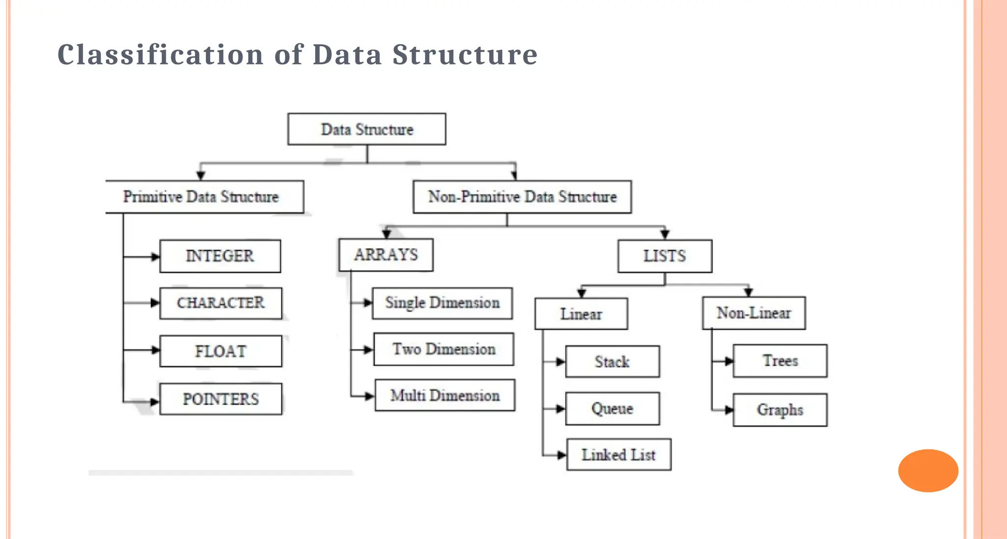
Primitive Data Structure
Thereare basic structures and directly operated upon by the machine
instructions.
Data structures that are directly operated upon the machine-level
instructions are known as primitive data structures.
Integer, Floating-point number, Character constants, string constants,
pointers etc, fall in this category.
The most commonly used operation on data structure are broadly
categorized into following types:
• Create
• Selection
• Updating
• Destroy or Delete
5.
NonPrimitive Data Structure
TheData structures that are derived from the primitive data structures are
called Non-primitive data structure.
The non-primitive data structures emphasize on structuring a group of
homogeneous (same type) or heterogeneous (different type) data items.
Linear Data structures: Non
Linear Data structures:
6.
Abstract Data Type(ADT)
ADT is a collection of data and a set of operations that can be performed on
the data.
It enables us to think abstractly about the data
We can separate concepts from implementation.
Typically, we choose a data structure and algorithms that provide an
implementation of an ADT.
7.
Linear List
□ Linearlist is a data object whose instances are of the form (e1 ,e2 ,...,
en )
□ ei is an element of the list.
□ e1 is the first element, and en is the last element.
□ n is the length of the list.
□ When n = 0, it is called an empty list.
□ e1 comes before e2 , e2 comes before e3 , and so on.
8.
Implementations of LinearList
Arraybased (Formulabased)
Uses a mathematical formula to determine where (i.e., the memory
address) to store each element of a list
Linked list (Pointerbased)
The elements of a list may be stored in any arbitrary set of locations
Each element has an explicit pointer (or link) to the next element
Indirect addressing
The elements of a list may be stored in any arbitrary set of locations
Maintain a table such that the ith table entry tells us where the ith
element is stored
Simulated pointer
Similar to linked representation but integers replace the C++ pointers
9.
Formulabased representation
A formula-basedrepresentation uses an array to represent the
instances of an object. Each position of the array, called a cell or a
node, holds one element that makes up an instance
of that object. Individual elements of an instance are located in the array,
based on a mathematical formula, e.g., a simple and often used formula
is
Location(i) = i − 1,
which says the ith
element of the list is in position i − 1. We also need
two more variables, length and MaxSize, to completely characterize
the list type.
10.
Linked lists
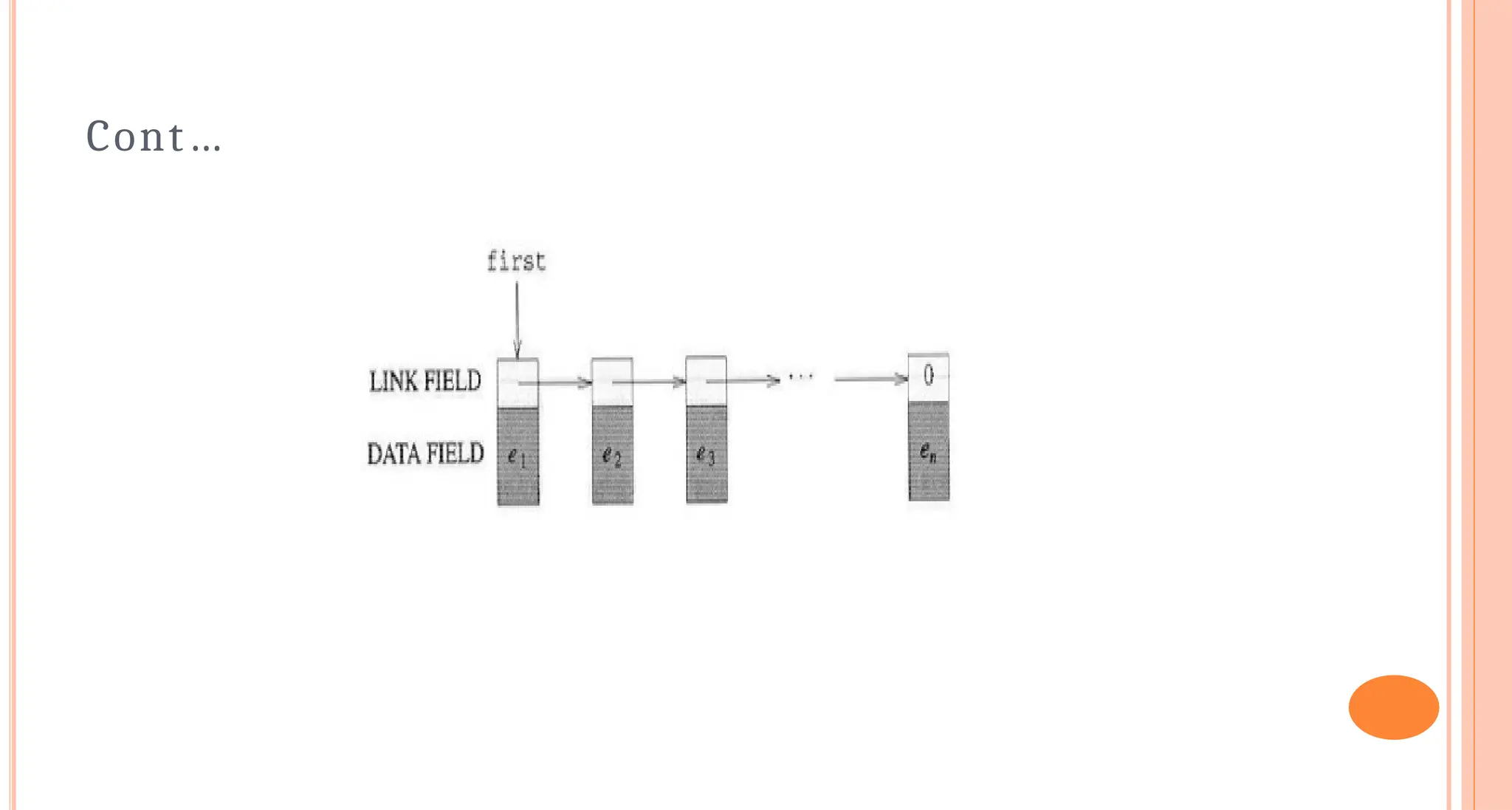
One wayto overcome the inefficiency problem of the previous approach is to
assign space on a need-only base. No space will be assigned if there is no
need; and whenever there is a need, another piece of space will be
assigned to an element. Since, we can’t guarantee all the pieces of spaces
assigned at different times will be physically adjacent, besides the space
assigned for the elements, we also have to keep track of the location
information of previously assigned pieces.
Hence, in a linked representation, each element of an instance is
presented in a cell or node, which also contains a pointer that keeps
information about the location of another node.
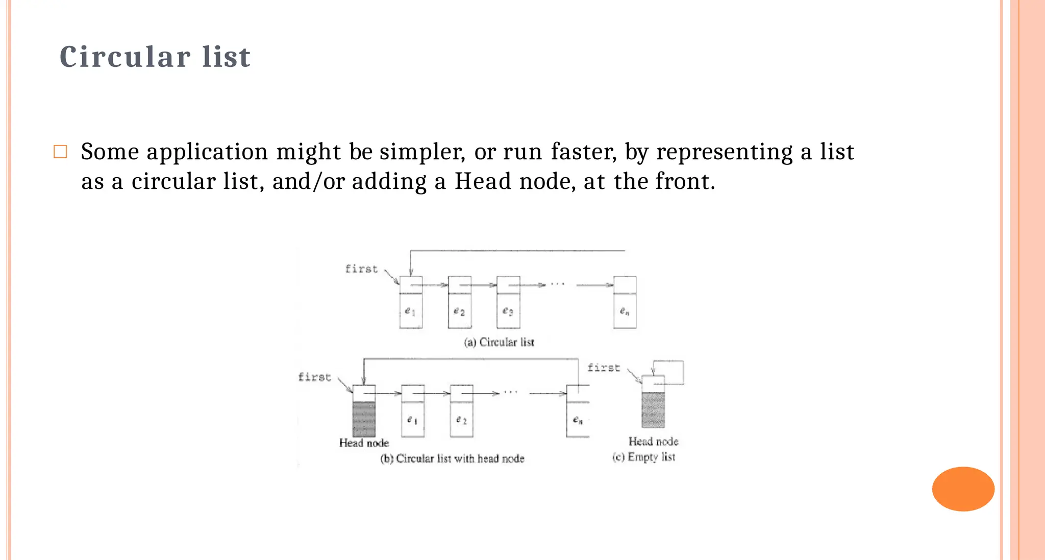
Circular list
□ Someapplication might be simpler, or run faster, by representing a list
as a circular list, and/or adding a Head node, at the front.
13.
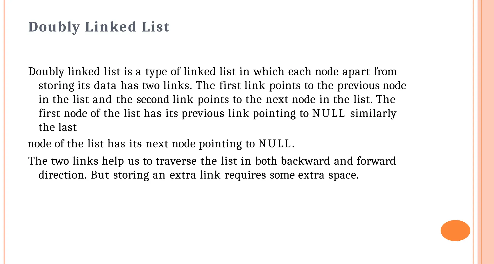
Doubly Linked List
Doublylinked list is a type of linked list in which each node apart from
storing its data has two links. The first link points to the previous node
in the list and the second link points to the next node in the list. The
first node of the list has its previous link pointing to NULL similarly
the last
node of the list has its next node pointing to NULL.
The two links help us to traverse the list in both backward and forward
direction. But storing an extra link requires some extra space.
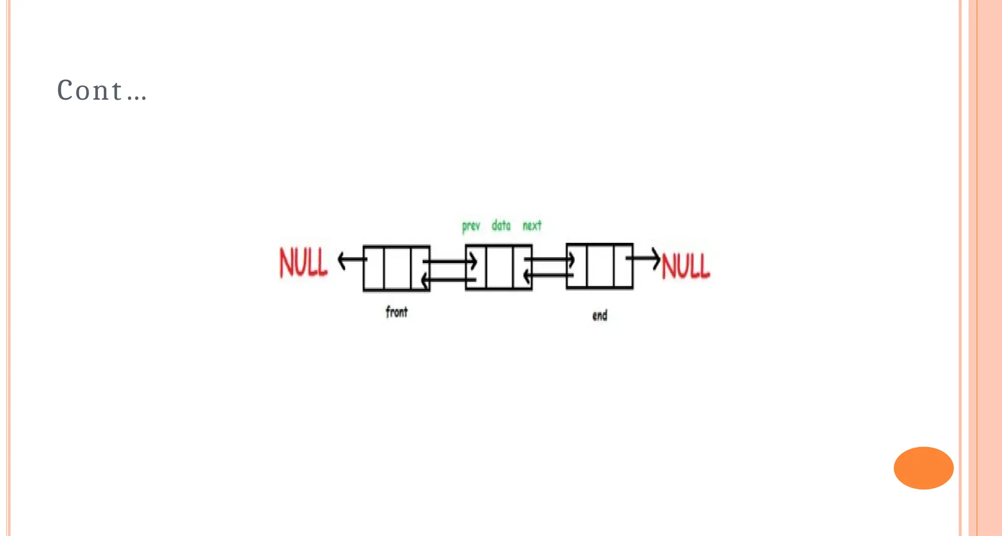
Indirect addressing
This approachcombines the formula-based approach and that of the
linked representation. As a result, we can not only get access to elements
in Θ(1) times, but also have the storage flexibility, elements will not be
physically moved during insertion and/or deletion.
In indirect addressing, we use a table of pointers to get access to a list of
elements, as shown in the following figure.
16.
Stacks
A stack isa container of objects that are inserted and removed according to
the last-in first-out (LIFO) principle. In the pushdown stacks only two
operations are allowed: push the item into the stack, and pop the item
out of the stack. A stack is a limited access data structure - elements can
be added and removed from the stack only at the top. push adds an item
to the top of the stack, pop removes the item from the top. A helpful
analogy is to think of a stack of books; you can remove only the top book,
also you can add a new book on the top.
17.
Cont…
Applications
The simplest applicationof a stack is to reverse a word. You push a given
word to stack - letter by letter - and then pop letters from the stack.
Another application is an "undo" mechanism in text editors; this
operation is accomplished by keeping all text changes in a stack.
18.
CONT…
Backtracking: This isa process when you need to access the most
recent data element in a series of elements. Think of a labyrinth or
maze - how do you find a way from an entrance to an exit?
Once you reach a dead end, you must backtrack. But backtrack to
where? to the previous choice point. Therefore, at each choice point you
store on a stack all possible choices.
Then backtracking simply means popping a next choice from the stack.
19.
Cont…
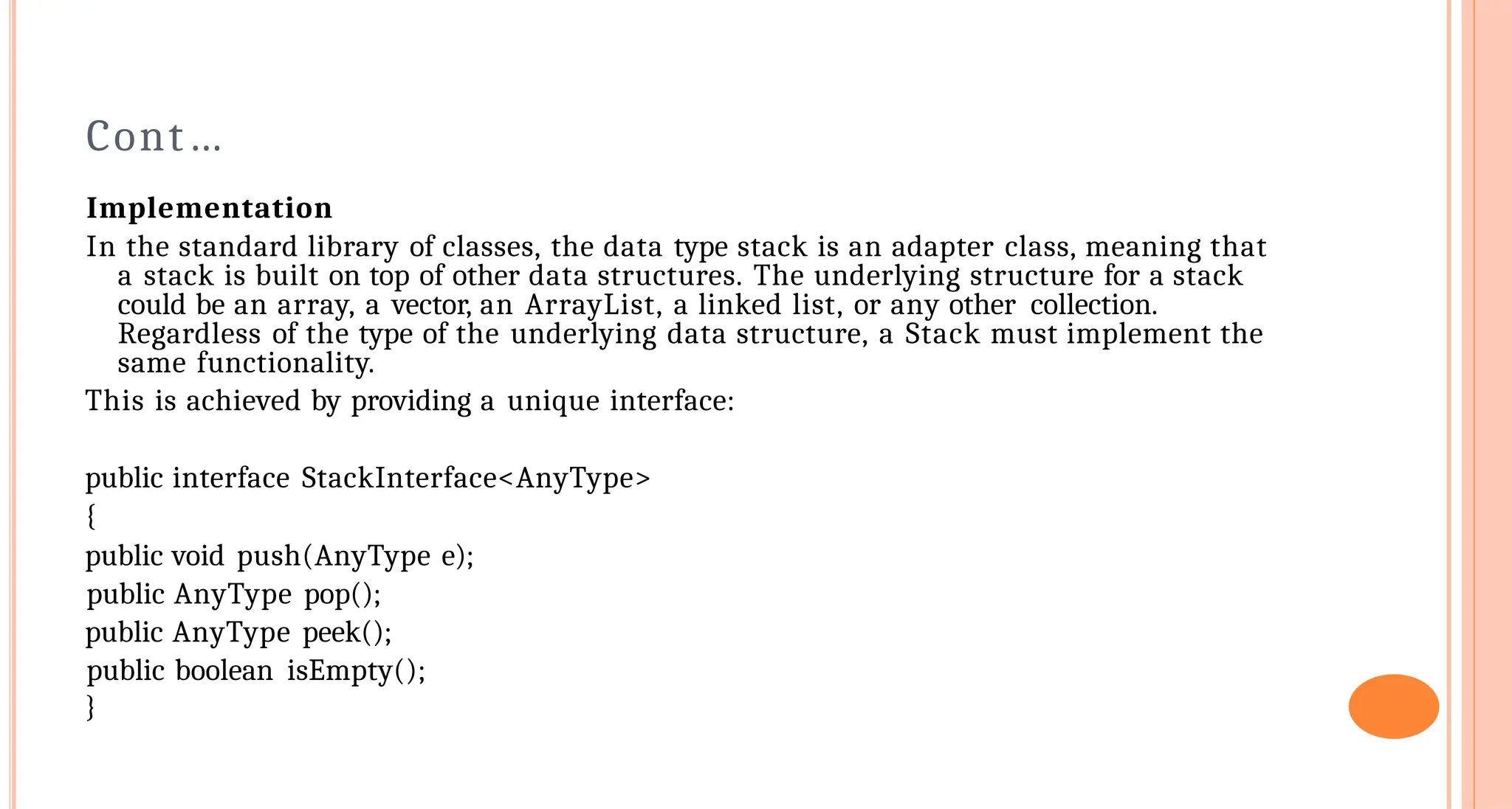
Implementation
In the standardlibrary of classes, the data type stack is an adapter class, meaning that
a stack is built on top of other data structures. The underlying structure for a stack
could be an array, a vector, an ArrayList, a linked list, or any other collection.
Regardless of the type of the underlying data structure, a Stack must implement the
same functionality.
This is achieved by providing a unique interface:
public interface StackInterface<AnyType>
{
public void push(AnyType e);
public AnyType pop();
public AnyType peek();
public boolean isEmpty();
}
20.
Cont…
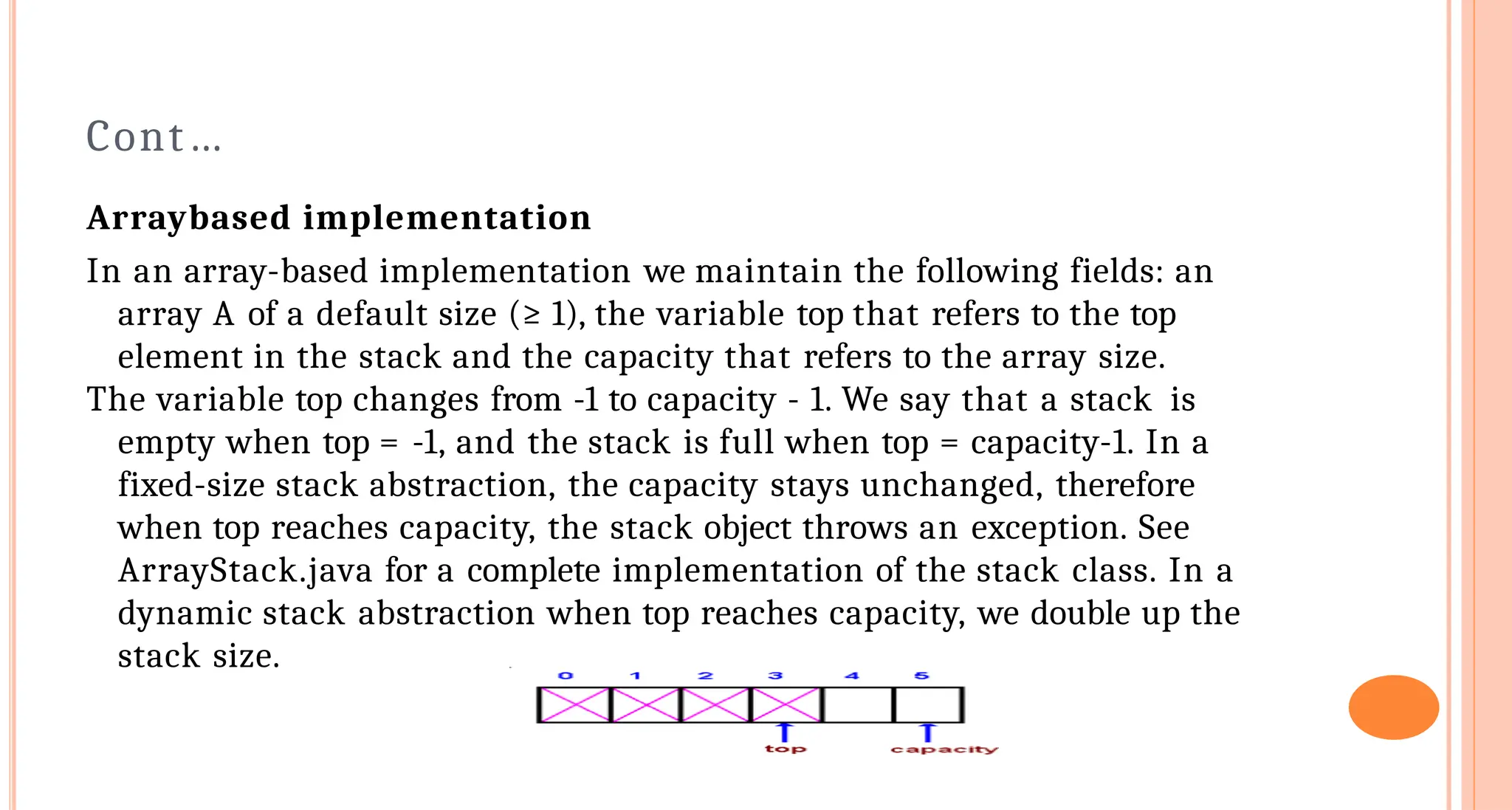
Arraybased implementation
In anarray-based implementation we maintain the following fields: an
array A of a default size (≥ 1), the variable top that refers to the top
element in the stack and the capacity that refers to the array size.
The variable top changes from -1 to capacity - 1. We say that a stack is
empty when top = -1, and the stack is full when top = capacity-1. In a
fixed-size stack abstraction, the capacity stays unchanged, therefore
when top reaches capacity, the stack object throws an exception. See
ArrayStack.java for a complete implementation of the stack class. In a
dynamic stack abstraction when top reaches capacity, we double up the
stack size.
21.
Cont…
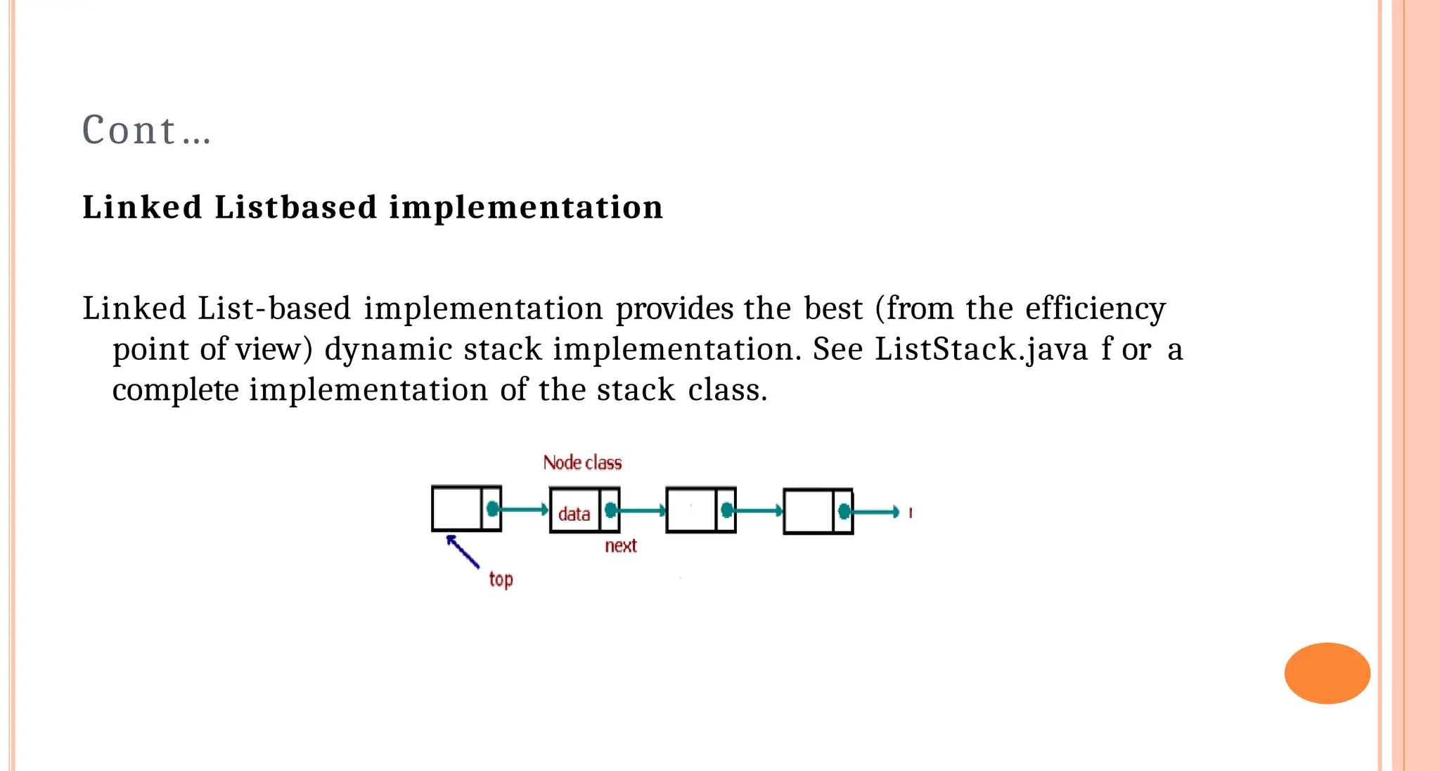
Linked Listbased implementation
LinkedList-based implementation provides the best (from the efficiency
point of view) dynamic stack implementation. See ListStack.java f or a
complete implementation of the stack class.
22.
Queues
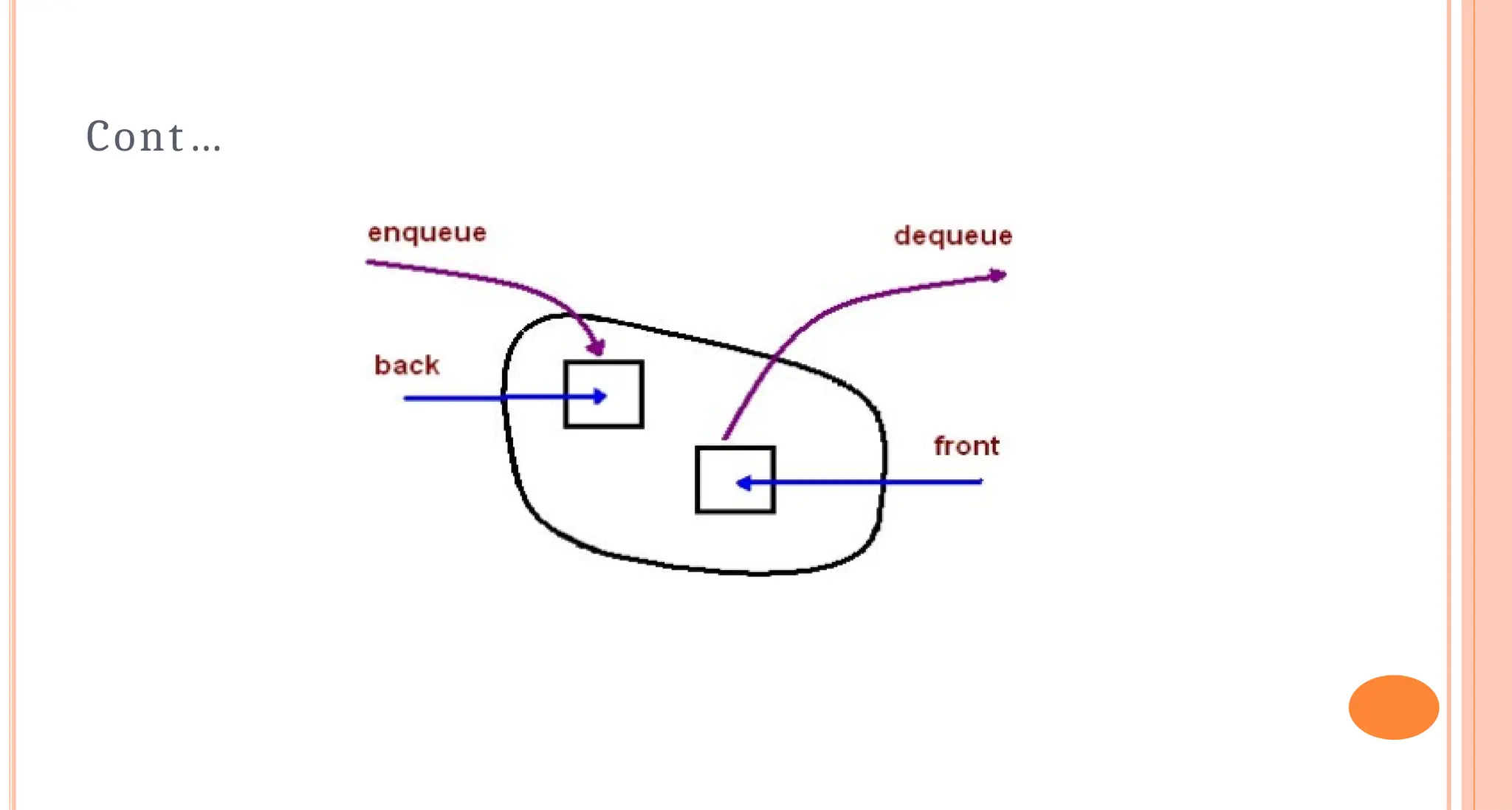
A queue isa container of objects (a linear collection) that are inserted and
removed according to the first-in first- out (FIFO) principle. An excellent
example of a queue is a line of students in the food court of the UC. New
additions to a line made to the back of the queue, while removal (or
serving) happens in the front. In the queue only two operations are
allowed enqueue and dequeue. Enqueue means to insert an item into the
back of the queue, dequeue means removing the front item. The picture
demonstrates the FIFO access. The difference between stacks and queues
is in removing. In a stack we remove the item the most recently added;
in a queue, we remove the item the least recently added.
Cont…
Implementation
In the standardlibrary of classes, the data type queue is an adapter class, meaning that a queue is built on
top of other data structures. The underlying structure for a queue could be an array, a Vector, an
ArrayList, a LinkedList, or any other collection. Regardless of the type of the underlying data structure,
a queue must implement the same functionality. This is achieved by providing a unique interface.
interface QueueInterface‹AnyType>
{
public boolean isEmpty();
public AnyType getFront();
public AnyType dequeue();
public void enqueue(AnyType e);
public void clear();
}
25.
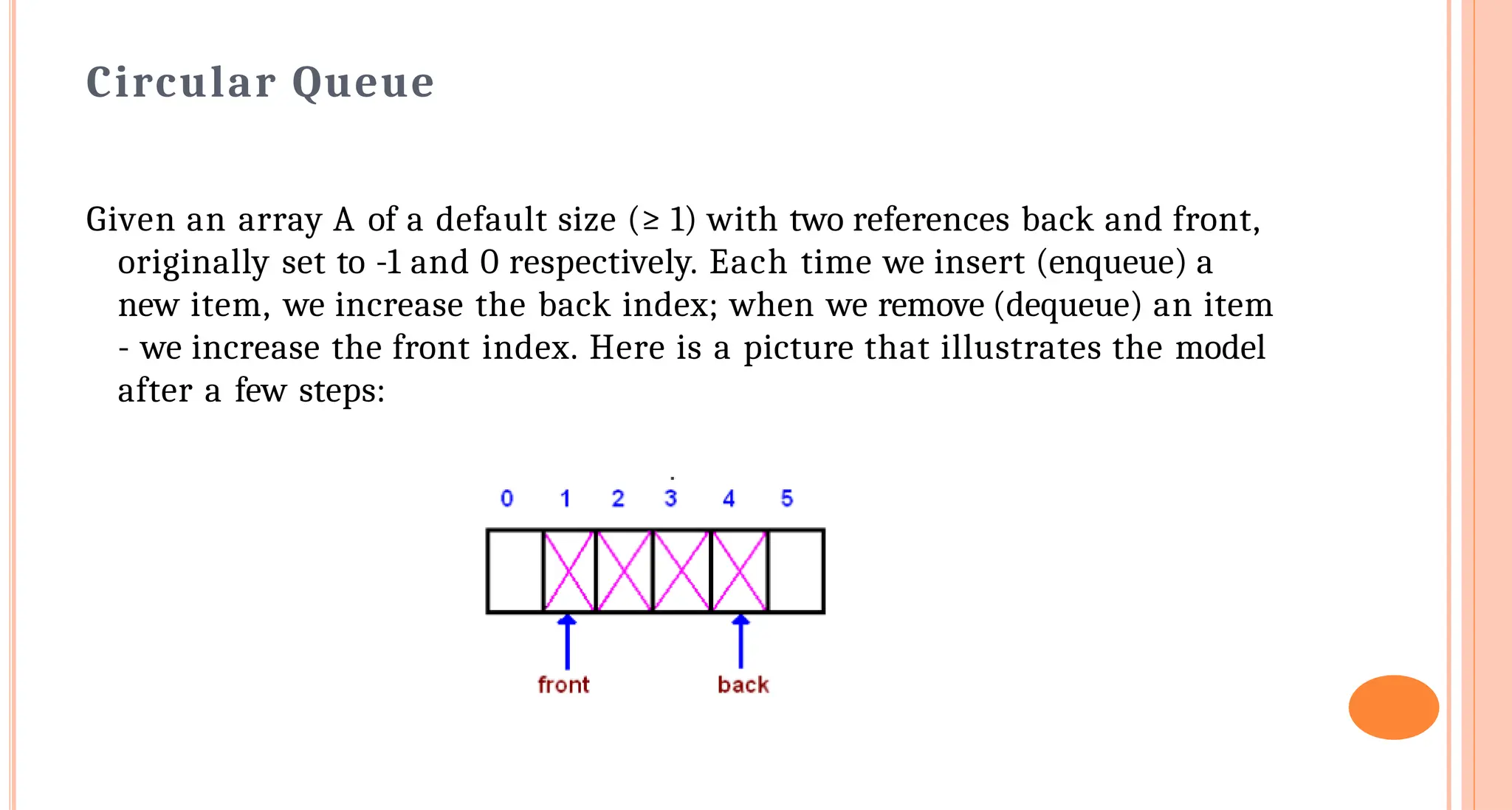
Circular Queue
Given anarray A of a default size (≥ 1) with two references back and front,
originally set to -1 and 0 respectively. Each time we insert (enqueue) a
new item, we increase the back index; when we remove (dequeue) an item
- we increase the front index. Here is a picture that illustrates the model
after a few steps:
26.
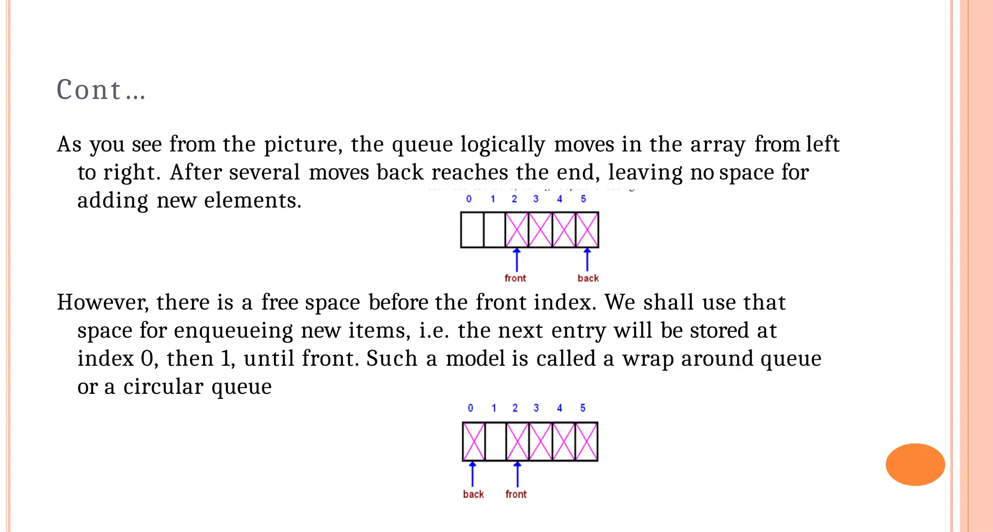
Cont…
As you seefrom the picture, the queue logically moves in the array from left
to right. After several moves back reaches the end, leaving no space for
adding new elements.
However, there is a free space before the front index. We shall use that
space for enqueueing new items, i.e. the next entry will be stored at
index 0, then 1, until front. Such a model is called a wrap around queue
or a circular queue
27.
Applications
The simplest twosearch techniques are known as Depth-First Search(DFS)
and Breadth-First Search (BFS). These two searches are described by
looking at how the search tree (representing all the possible paths from
the start) will be traversed.
28.
DeapthFirst Search witha Stack
In depth-first search we go down a path until we get to a dead end; then we
backtrack or back up (by popping a stack) to get an alternative path.
• Create a stack
• Create a new choice point
• Push the choice point onto the stack
• while (not found and stack is not empty)
o Pop the stack
o Find all possible choices after the last one tried
o Push these choices onto the stack
• Return
29.
BreadthFirst Search witha Queue
In breadth-first search we explore all the nearest possibilities by finding all
possible successors and enqueue them to a queue.
• Create a queue
• Create a new choice point
• Enqueue the choice point onto the queue
• while (not found and queue is not empty)
o Dequeue the queue
o Find all possible choices after the last one tried
o Enqueue these choices onto the queue
• Return
30.
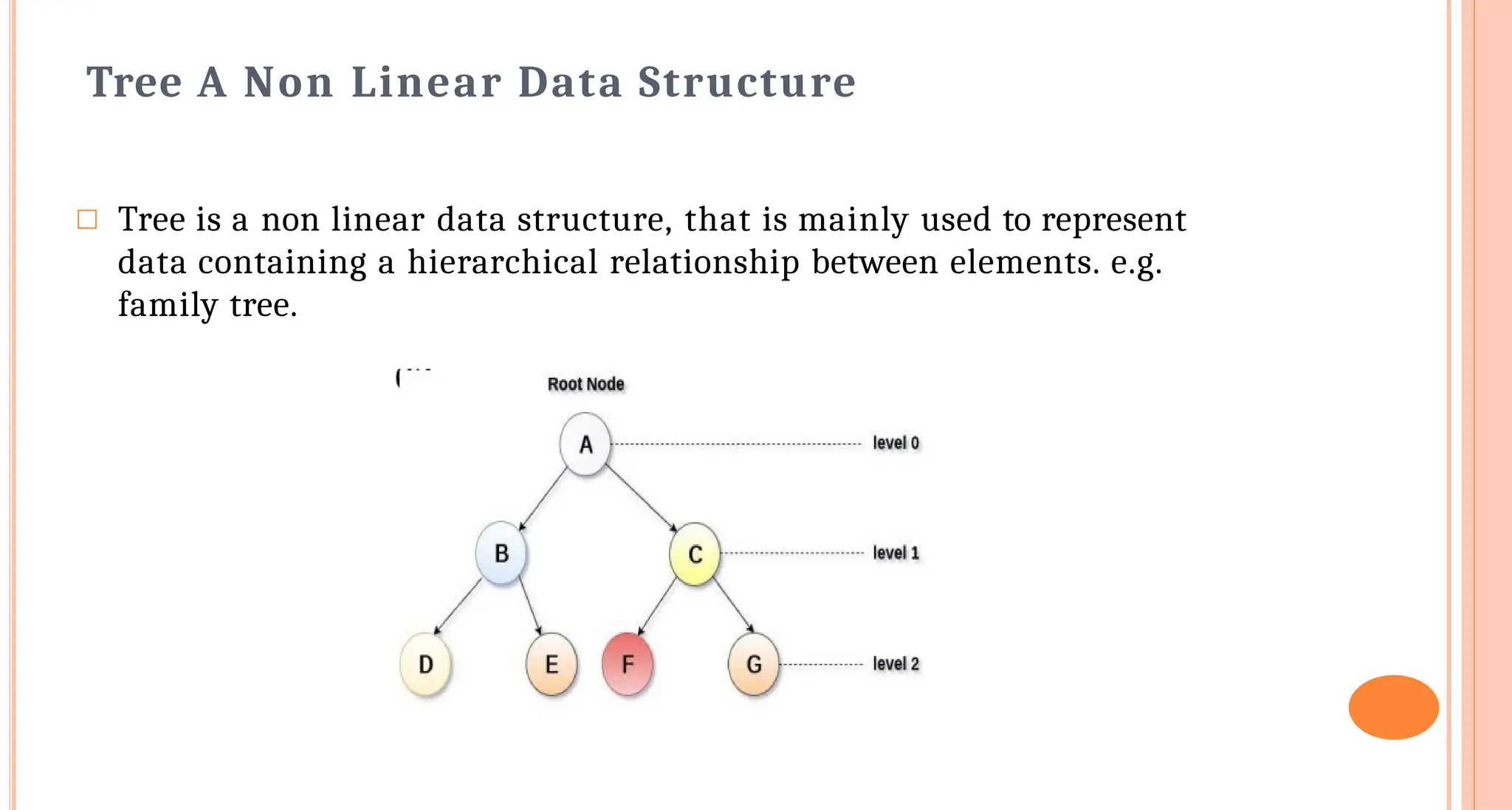
TreeA Non LinearData Structure
□ Tree is a non linear data structure, that is mainly used to represent
data containing a hierarchical relationship between elements. e.g.
family tree.
31.
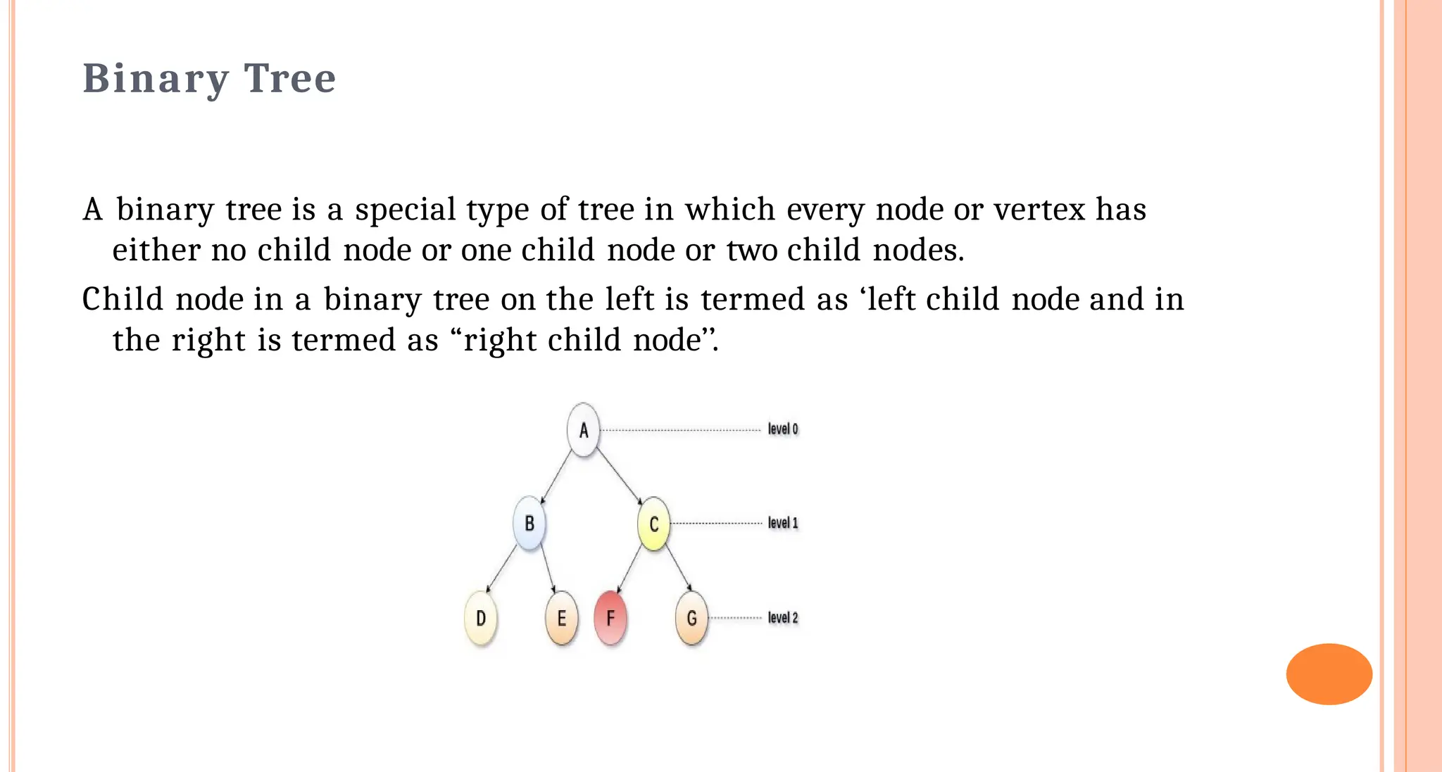
Binary Tree
A binarytree is a special type of tree in which every node or vertex has
either no child node or one child node or two child nodes.
Child node in a binary tree on the left is termed as ‘left child node and in
the right is termed as “right child node’’.
32.
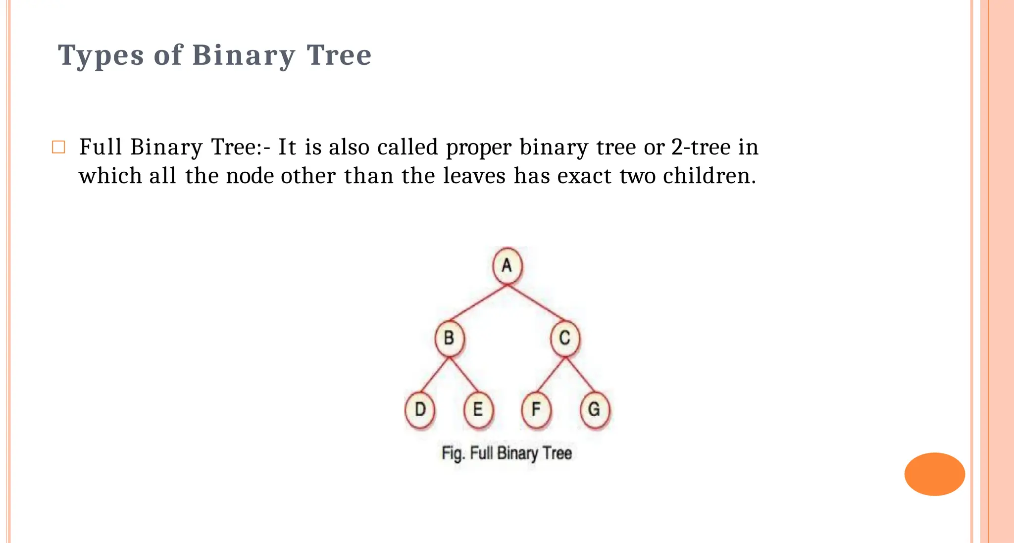
Types of BinaryTree
□ Full Binary Tree:- It is also called proper binary tree or 2-tree in
which all the node other than the leaves has exact two children.
33.
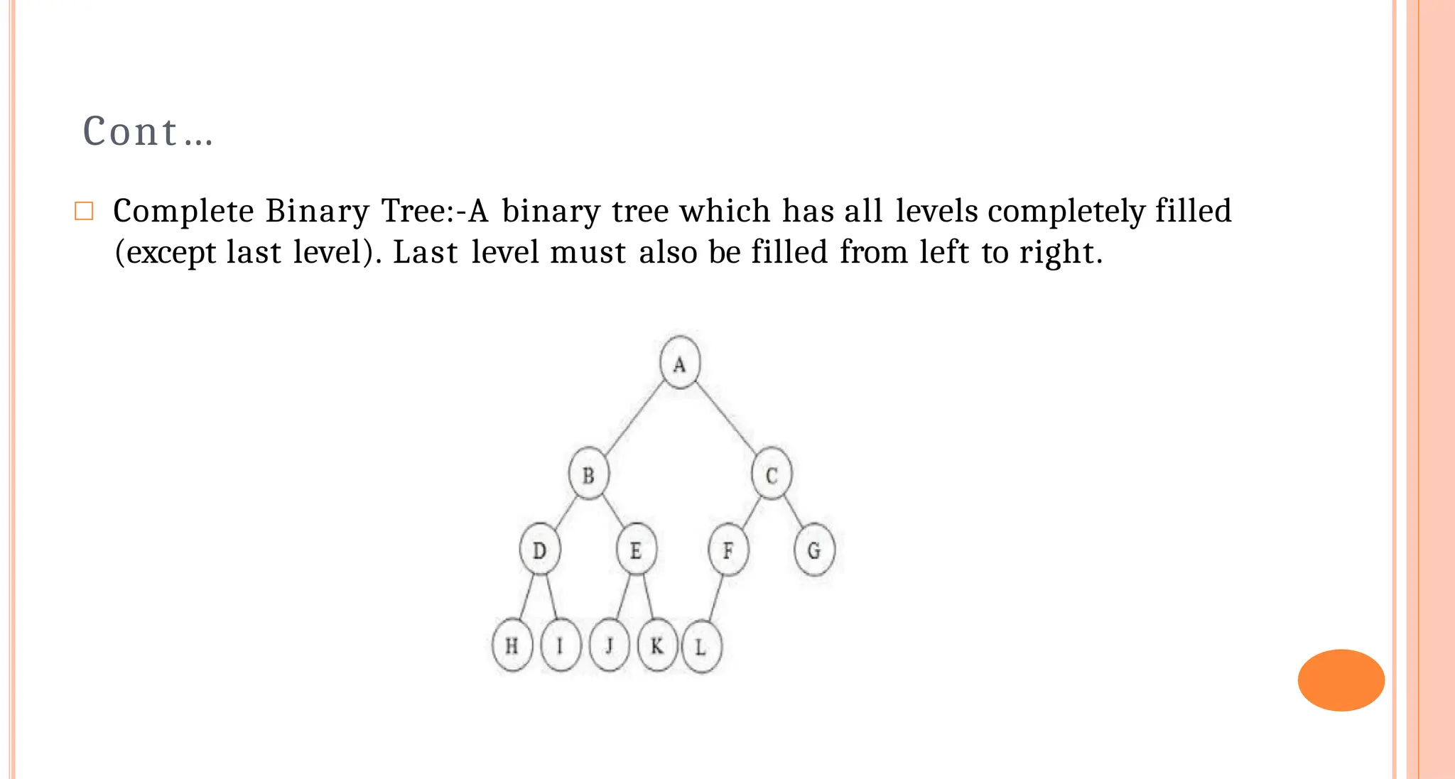
Cont…
□ Complete BinaryTree:-A binary tree which has all levels completely filled
(except last level). Last level must also be filled from left to right.
34.
Cont…
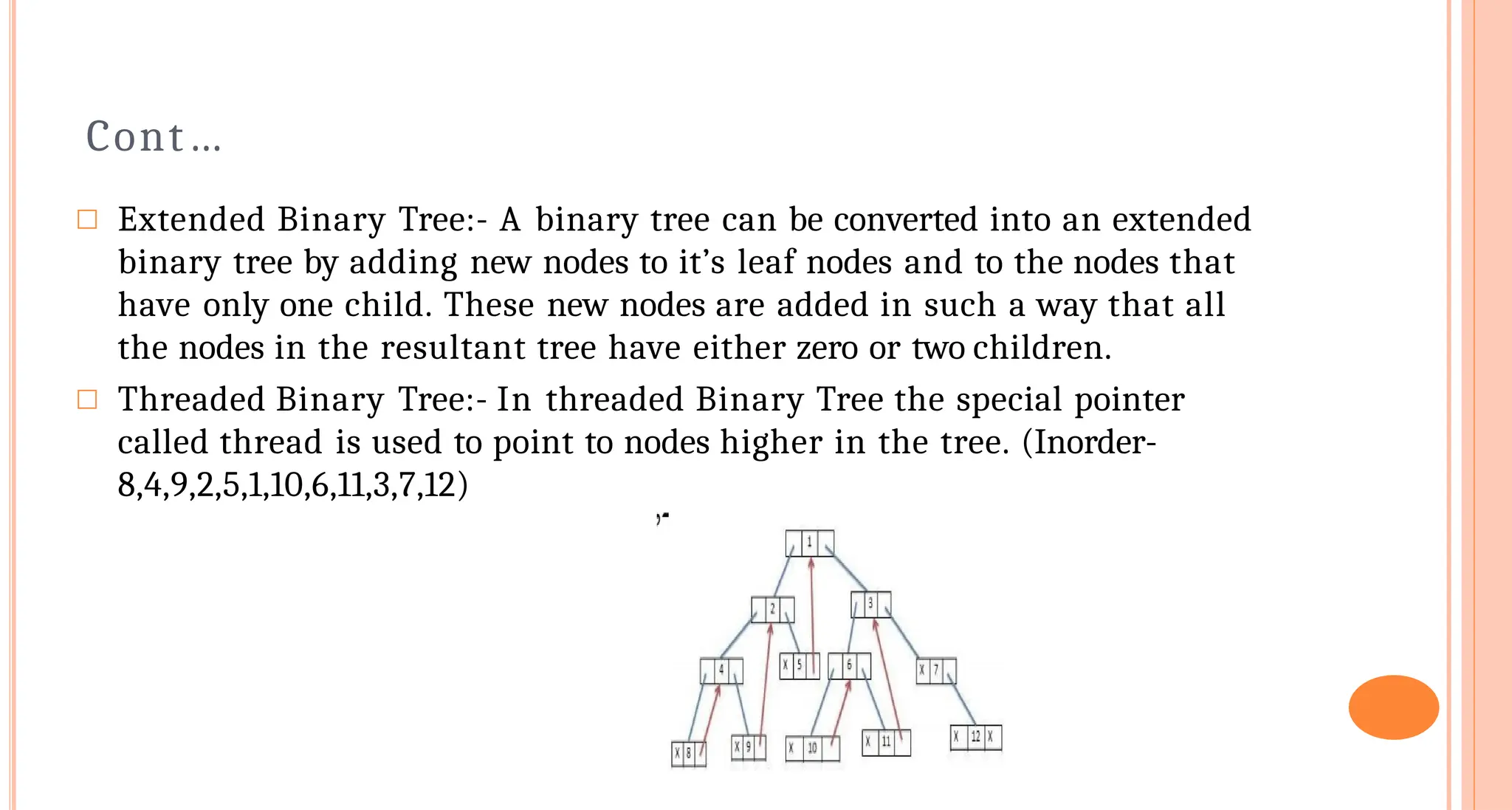
□ Extended BinaryTree:- A binary tree can be converted into an extended
binary tree by adding new nodes to it’s leaf nodes and to the nodes that
have only one child. These new nodes are added in such a way that all
the nodes in the resultant tree have either zero or two children.
□ Threaded Binary Tree:- In threaded Binary Tree the special pointer
called thread is used to point to nodes higher in the tree. (Inorder-
8,4,9,2,5,1,10,6,11,3,7,12)
35.
Memory Representation ofBinary Tree
1. Array Representation of Binary Tree:-
(i)Root is stored in a[0]
(ii)Node occupies- a[i]
• Left child-[2*i+1]
• Right child-[2*i+2]
• Parent node-[(i-1)/2]
36.
Cont…
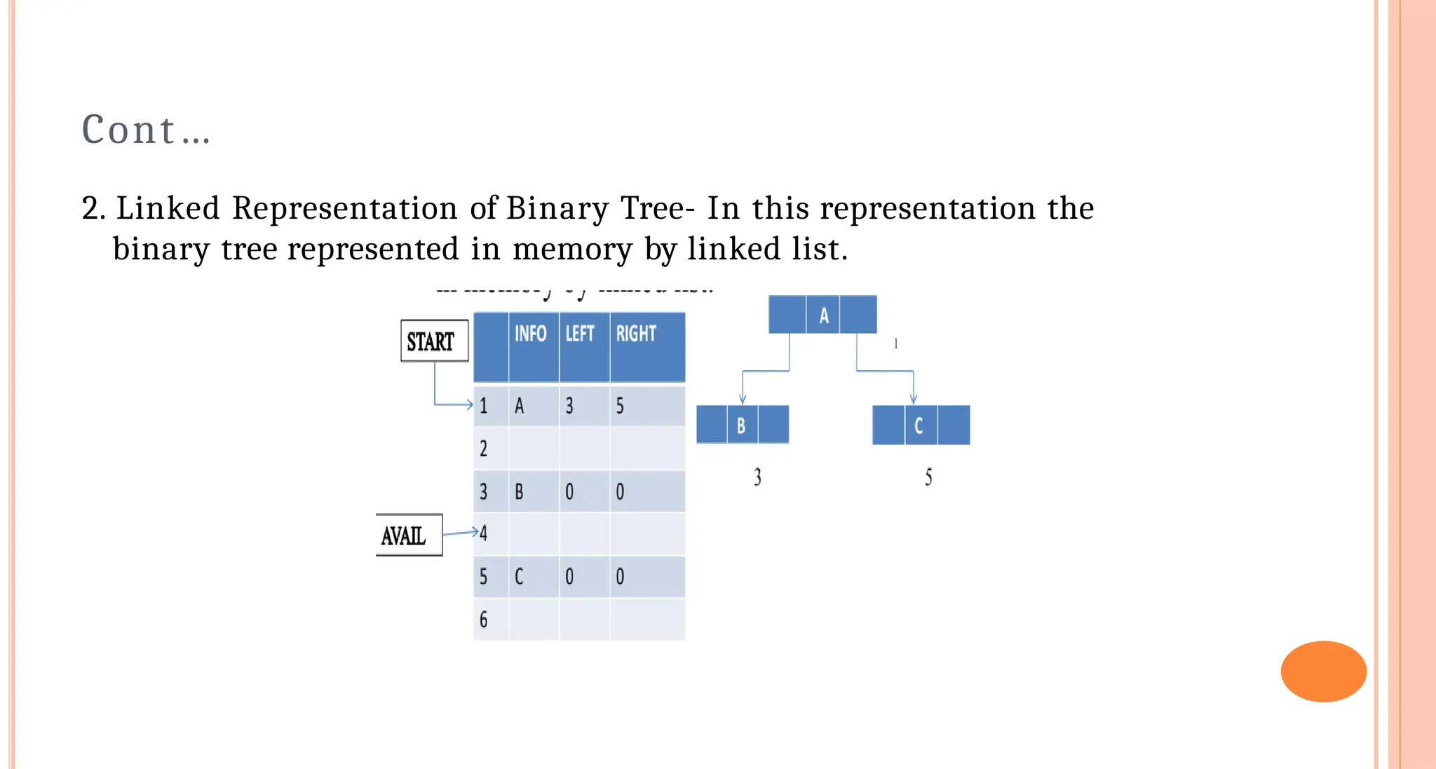
2. Linked Representationof Binary Tree- In this representation the
binary tree represented in memory by linked list.
37.
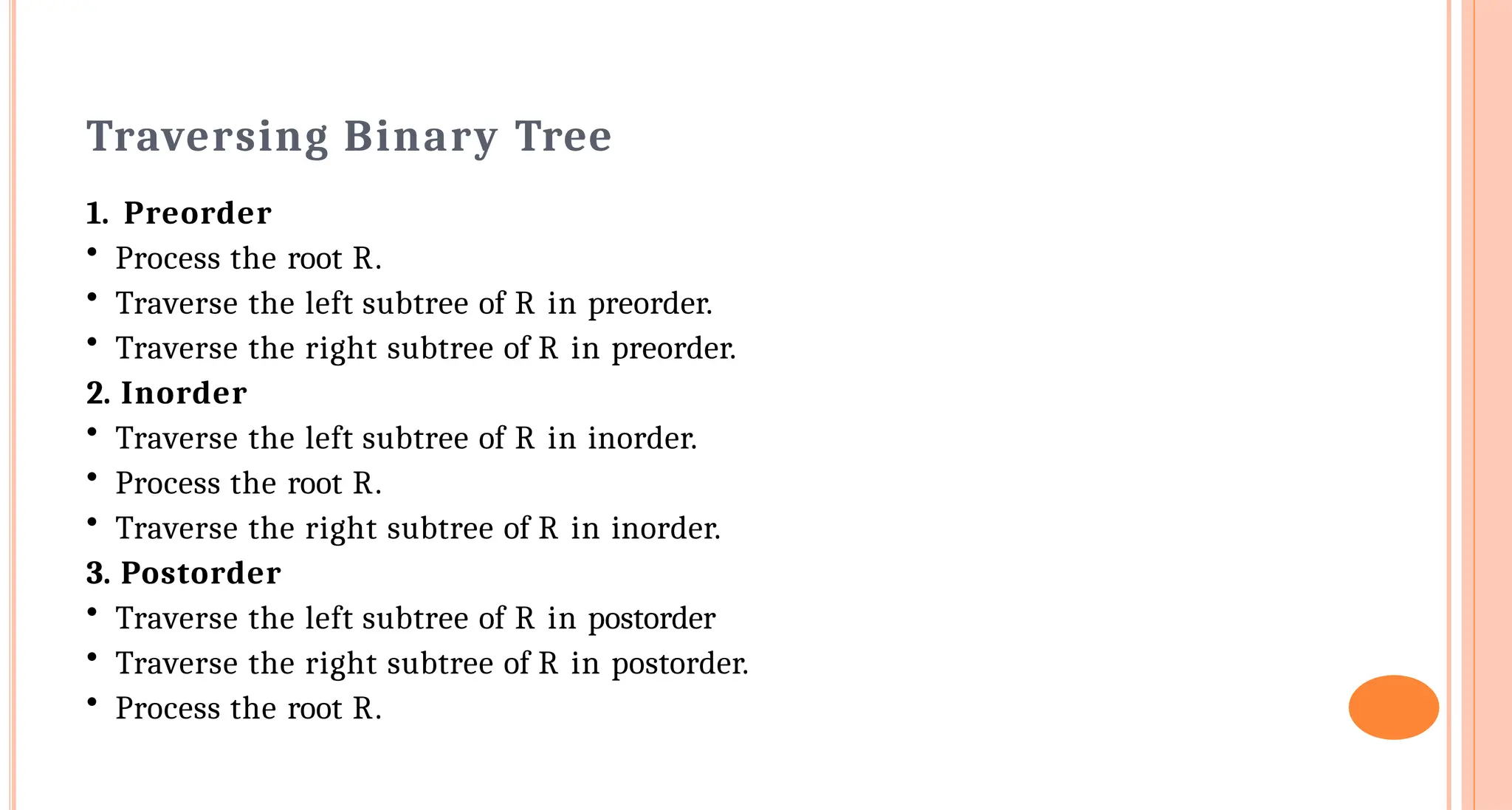
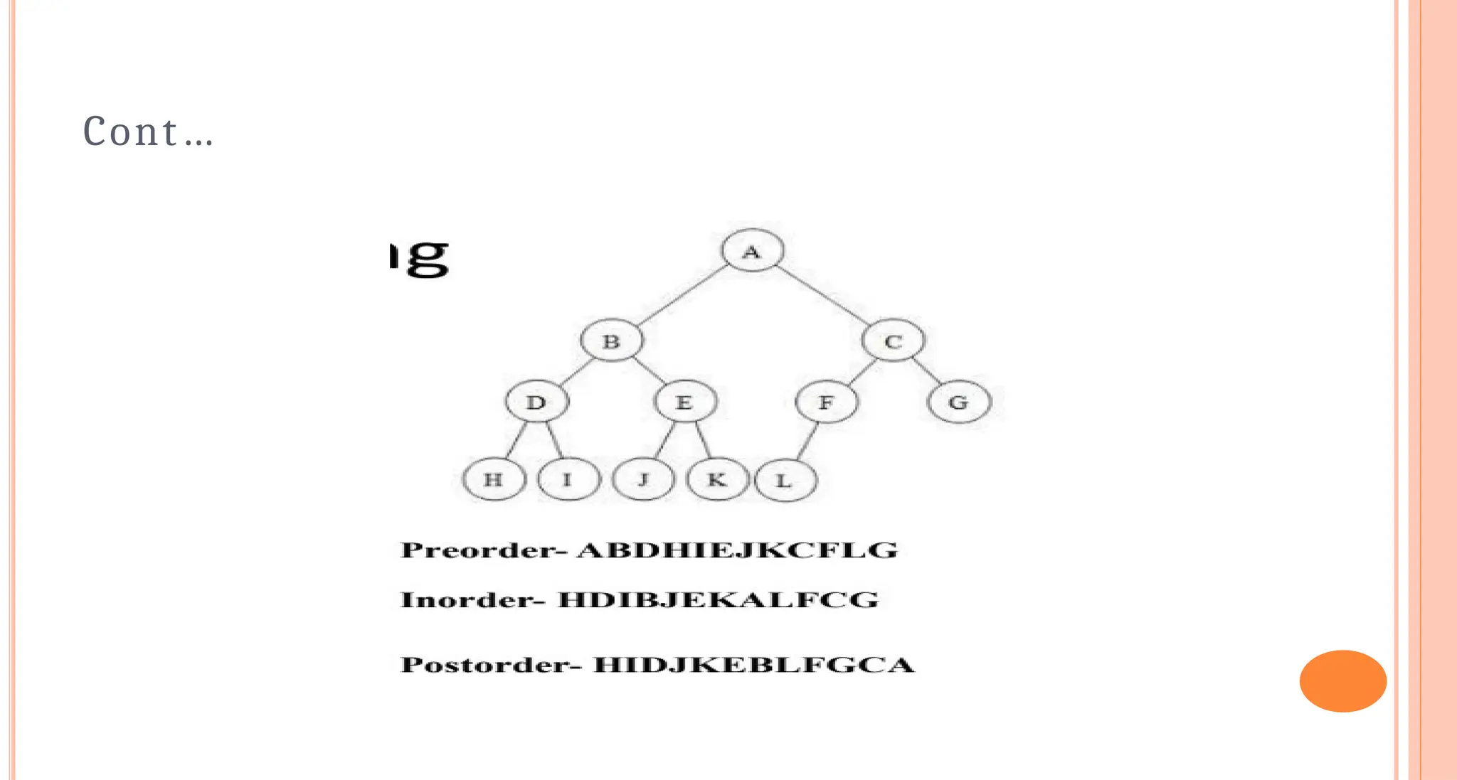
Traversing Binary Tree
1.Preorder
• Process the root R.
• Traverse the left subtree of R in preorder.
• Traverse the right subtree of R in preorder.
2. Inorder
• Traverse the left subtree of R in inorder.
• Process the root R.
• Traverse the right subtree of R in inorder.
3. Postorder
• Traverse the left subtree of R in postorder
• Traverse the right subtree of R in postorder.
• Process the root R.
PREORD(INFO, LEFT, RIGHT,ROOT)
A binary tree T is in memory. The algorithm does a preorder traversal of T, applying an
operation PROCESS to each of its nodes. An array STACK is used to temporarily hold
the addresses of nodes.
1. [Initially push NULL onto STACK, and initialize PTR.]
Set TOP := 1, STACK[1] := NULL and PTR := ROOT.
2. Repeat Steps 3 to 5 while PTR = NULL:
3. Apply PROCESS to INFO[PTR].
4. [Right child?]
If RIGHT[PTR] = NULL, then: [Push on STACK.]
Set TOP := TOP + 1, and STACK[TOP] := RIGHT[PTR].
[End of If structure.]
5.[Left child?]
If LEFT[PTR] NULL, then:
Set PTR := LEFT[PTR].
Else: [Pop from STACK.]
Set PTR := STACK[TOP]
and TOP := TOP - 1.
[End of If structure.]
[End of Step 2 loop.]
6. Exit.
40.
INORD(INFO, LEFT, RIGHT,ROOT)
A binary tree is in memory. This algorithm does an inorder traversal of T, applying an operation
PROCESS to each of its nodes. An array STACK is used to temporarily hold the addresses of
nodes.
1. [Push NULL onto STACK and initialize PTR.]
Set TOP := 1, STACK[1] NULL and PTR := ROOT.
2. Repeat while PTR = NULL: (Pushes left-most path onto STACK.]
(a) Set TOP := TOP + 1 and STACK[TOP] := PTR. [Saves node.]
(b) Set PTR := LEFT[PTR). [Updates PTR.]
[End of loop.]
3. Şet PTR := STACK[TOP] and TOP := TOP - 1. [Pops node from
STACK.]
4. Repeat Steps 5 to 7 while PTR = NULL: [Backtracking.]
5. Apply PROCESS to INFO[PTR].
6. [Right child?] If RIGHT[PTR] # NULL, then:
(a) Set PTR := RIGH[PTR].
(b)Go to Step 2
[End of If structure.]
7. Set PTR :=
STACK[TOP] and
TOP := TOP -1. [Pops
node.]
[End of Step 4 loop.]
8. Exit.
41.
POSTORD(INFO, LEFT, RIGHT,ROOT)
A binary tree T is in memory. This algorithm does a postorder traversal of T. applying an operation PROCESS to each
of its nodes. An array STACK is used to temporarily hold the addresses of nodes.
1. [Push NULL onto STACK and initialize PTR.]
Set TOP := 1. STACK[1] := NULL and PTR := ROOT.
2. [Push left-most path onto STACK]
Repeat Steps 3 to 5 while PTR
NULL:
3. Set TOP := TOP + 1 and
STACK[TOP] := PTR.
[Pushes PTR on STACK]
4. If RIGHT[PTR] NULL, then: [Push on
STACK.]
Set TOP := TOP + 1 and
STACK[TOP] := -RIGHT[PTR].
[End of If structure.)
5. Set PTR := LEFT[PTR]. [Updates pointer PTR.]
[End of Step 2 loop.)
6. Set PTR := STACK[TOP] and TOP := TOP - 1.
[Pops node from STACK.]
7. Repeat while PTR > 0:
(a) Apply PROCESS to INFO[PTR).
(b) Set PTR := STACK[TOP] and TOP := TOP - 1.
[Pops node from STACK.]
[End of loop.]
8. If PTR <0, then:
42.
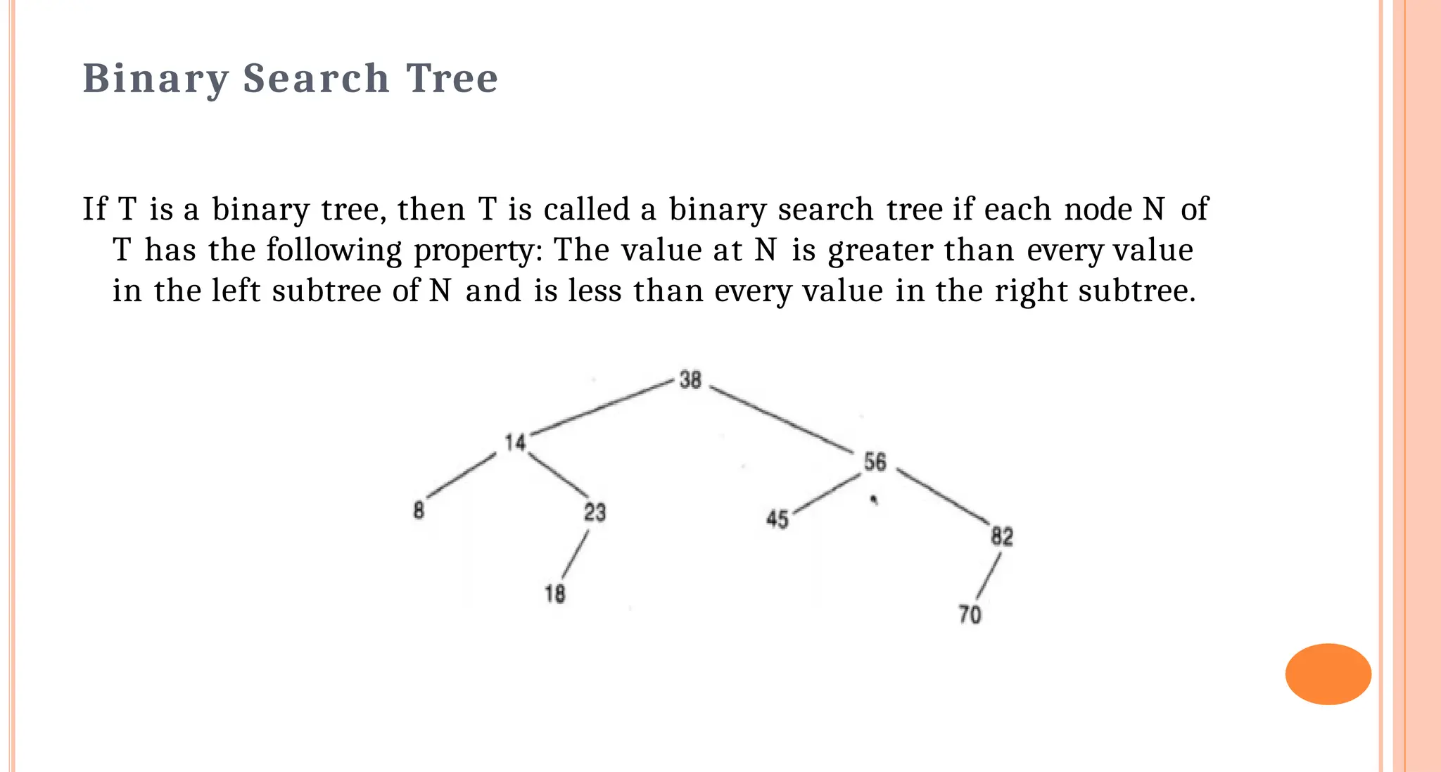
Binary Search Tree
IfT is a binary tree, then T is called a binary search tree if each node N of
T has the following property: The value at N is greater than every value
in the left subtree of N and is less than every value in the right subtree.
43.
Cont…
Searching & Inserting
Ifan ITEM of information is given. The following algorithm finds the
location of ITEM in the binary search tree T, or inserts ITEM as a
new node in its appropriate place in the tree.
(a) Compare ITEM with the root node N of the tree.
(i) IF ITEM <N, proceed to the left child of N.
(ii) If ITEM > N. proceed to the right child of N.
(b) Repeat Step (a) until one of the following occurs:
(i)We meet a node N such that ITEM = N. In this case the search Is
successful.
(ii)We meet an empty subtree, which indicates that the search is
unsuccessful, and we insert ITEM in place of the empty subtree.
Algo. For LocationFinding
FIND(INFO, LEFT. RIGHT, ROOT. ITEM, LOC, PAR)
A binary search tree T is in memory and an ITEM of information is given. This procedure finds the location LOC of
ITEM in T and also the location PAR of the parent of ITEM. There are three special cases:
(i) LOC = NULL and PAR - NULL will indicate that the tree is empty.
(ii) LOC NULL and PAR - NULL will indicate that ITEM is the root of T.
(iii) LOC = NULL and PAR = NULL will indicate that ITEM is not in T and can be added to T as a child of the node N
with location PAR.
1. [Tree empty?]
If ROOT = NULL, then: Set LOC := NULL and PAR := NULL. And Return.
2. [ITEM at root?]
If ITEM - INFO[ROO]), then: Set LOC := ROOT and PAR = NULL, and Return.
3. [Initialize pointers PTR and SAVE.]
If ITEM <INFO[ROOT]), then:
Set PTR := LEFT[ROOT] and SAVE := ROOT.
Else:
Set PTR := RIGHT[ROOT] and SAVE := ROOT
[End of If structure.]
4. Repeat Steps 5 and 6 while PTR ≠ NULL.
5. [ITEM found?]
If ITEM = INFO[PTR], then: Set LOC := PTR and PAR := SAVE and Return.
6. IF ITEM < INFO[PTR], then:
Set SAVE := PTR and PTR := LEFT[PTR].
Else:
Set SAVE := PTR and PTR := RIGHT[PTR].
[End of If structure.]
[End of Step 4 loop.]
7. [Search unsuccessful.] Set LOC:= NULL and PAR := SAVE.
8. Exit.
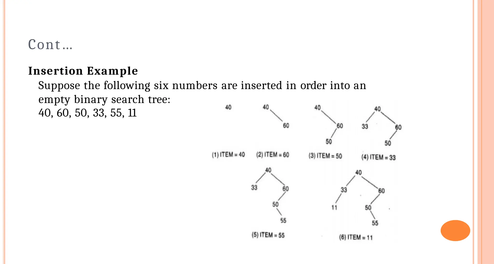
46.
Insertion Algo. ForBST
INSBST(INFO, LEFT, RIGHT, ROOT, AVAIL, ITEM, LOC)
A binary search tree T is in memory and an ITEM of information is given. This algorithm finds the
location LOC of ITEM in T or adds ITEM as a new node in T at location LOC.
1. Call FIND(INFO, LEFT, RIGHT, ROOT, ITEM, LOC, PAR).
[Procedure 7.4.)
2. If LOC ≠ NULL, then Exit.
3. [Copy ITEM into new node in AVAIL list.]
(a) IF AVAIL = NULL, then: Write: OVERFLOW, and Exit.
(b) Set NEW = AVAIL, AVAIL :=
LEFT[AVAIL] and INFO[NEW] := ITEM.
(c) Set LOC := NEW. LEFT[NEW] := NULL and
RIGHT[NEW] := NULL.
4. [Add ITEM to tree.]
If PAR = NULL, then:
Set ROOT := NEW.
Else if ITEM < INFO[PAR], then:
Set LEFT[PAR] := NEW.
Else:
Set RIGHT[PAR] := NEW.
[End of If structure.]
5. Exit.
47.
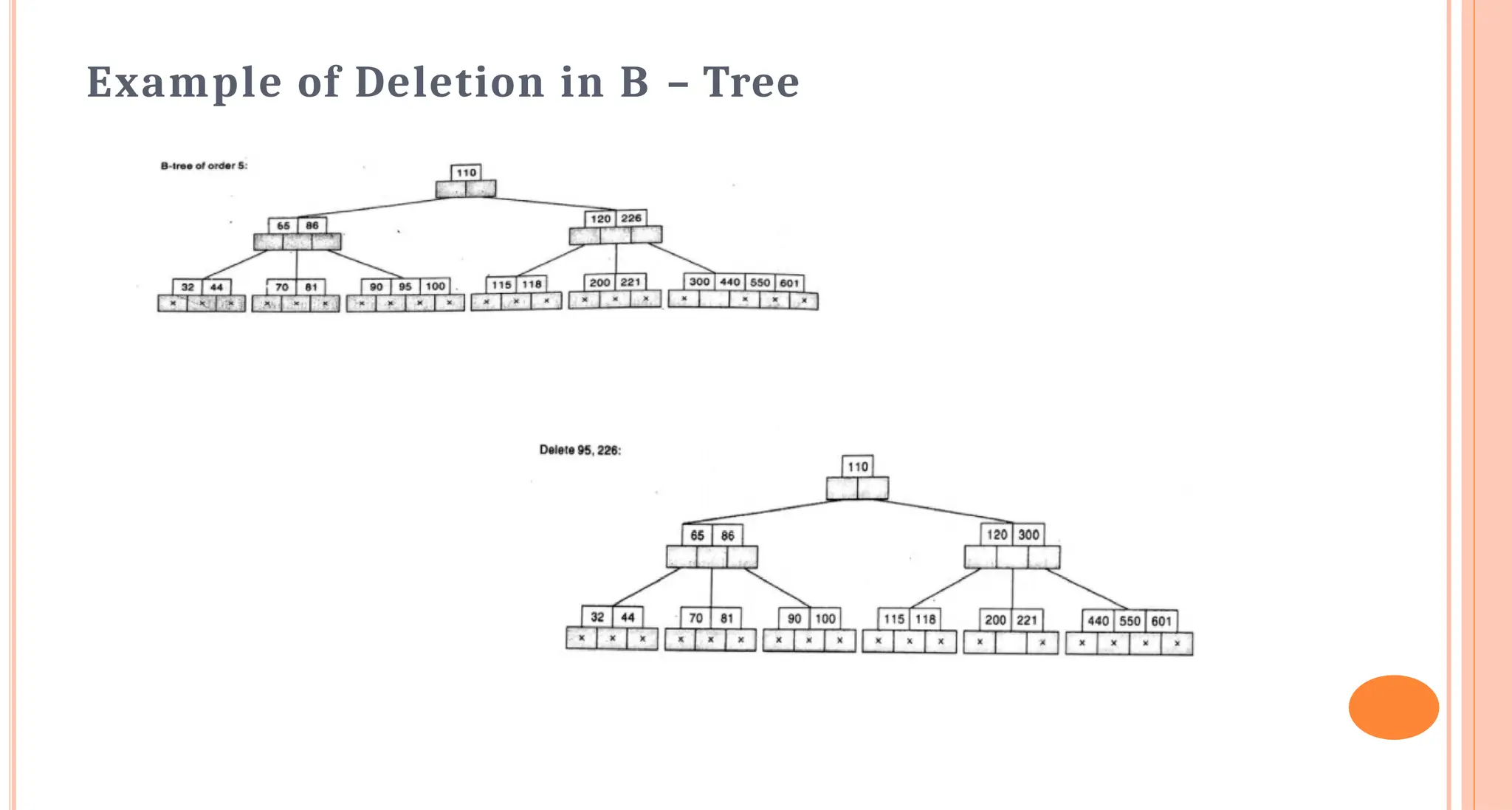
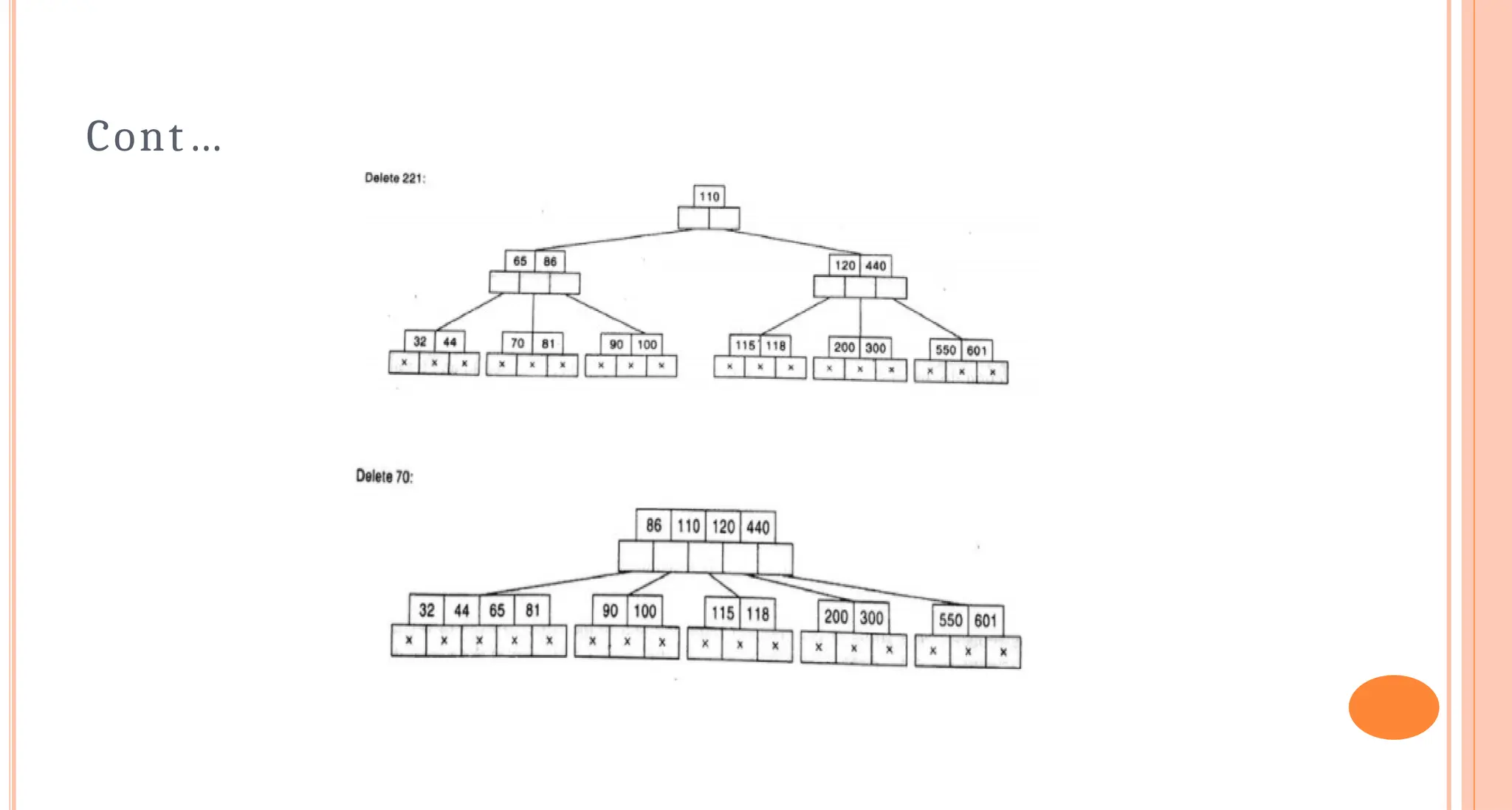
Deletion Algo. ForBST
If T is a BST, and an ITEM of information is given, then find the location of the node N
which contains ITEM and also the location of the parent node P(N). The way N is
deleted from the tree depends primarily on the number of children of node N. There
are three cases:
Case 1. N has no children. Then N is deleted from T by simply replacing the location of
N in the parent node P(N) by the null pointer.
Case 2. N has exactly one child. Then N is deleted froin T by simply replacing the
location of N in P(N) by the location of the only child of N.
Case 3. N has two children. Let S(N) denote the inorder successor of N. (The reader can
verify that S(N) does not have a left child.) Then N is deleted from T by first deleting
S(N) from T (by using Case 1 or Case 2) and then replacing node N in T by the node
S(N).
Observe that the third case is much more complicated than the first two cases. In all
three cases, the memory space of the deleted node N is returned to the AVAIL list.
48.
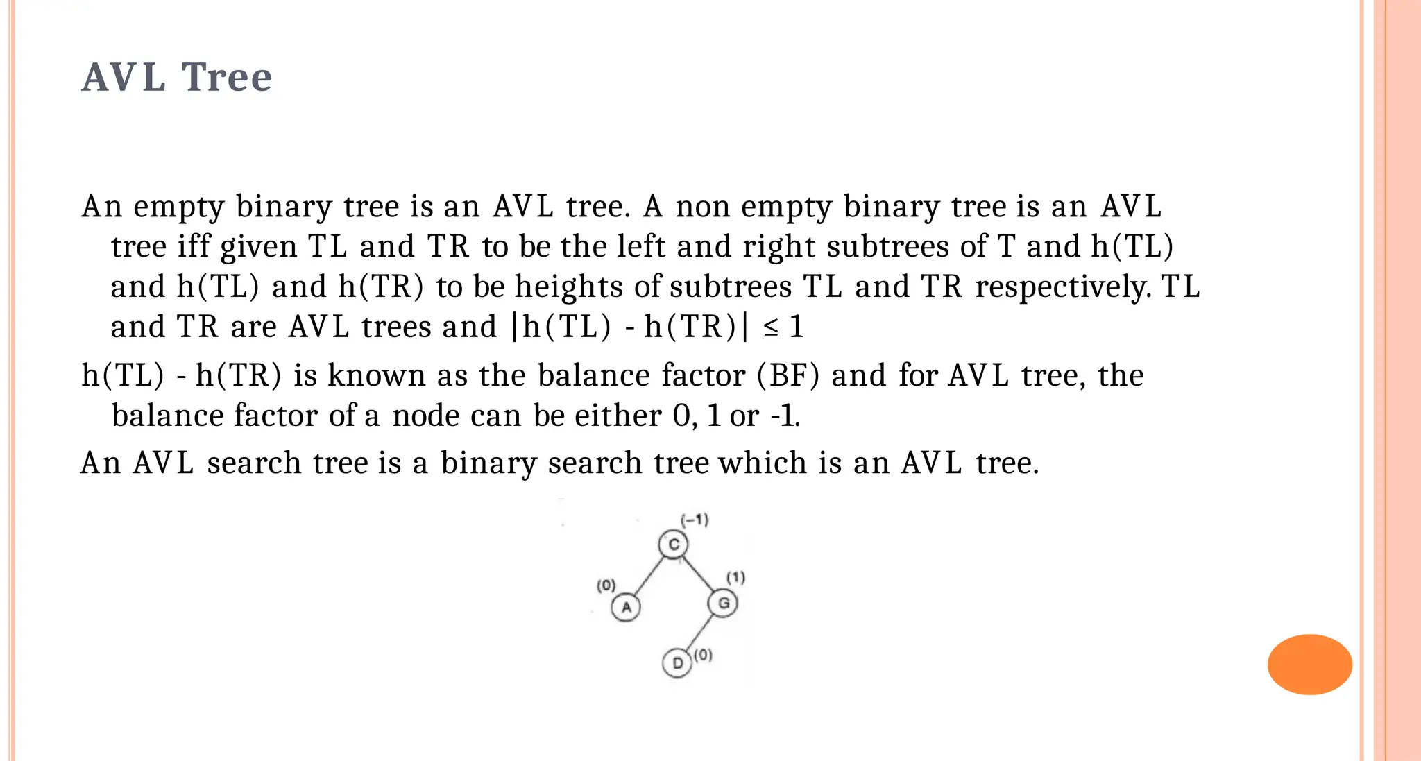
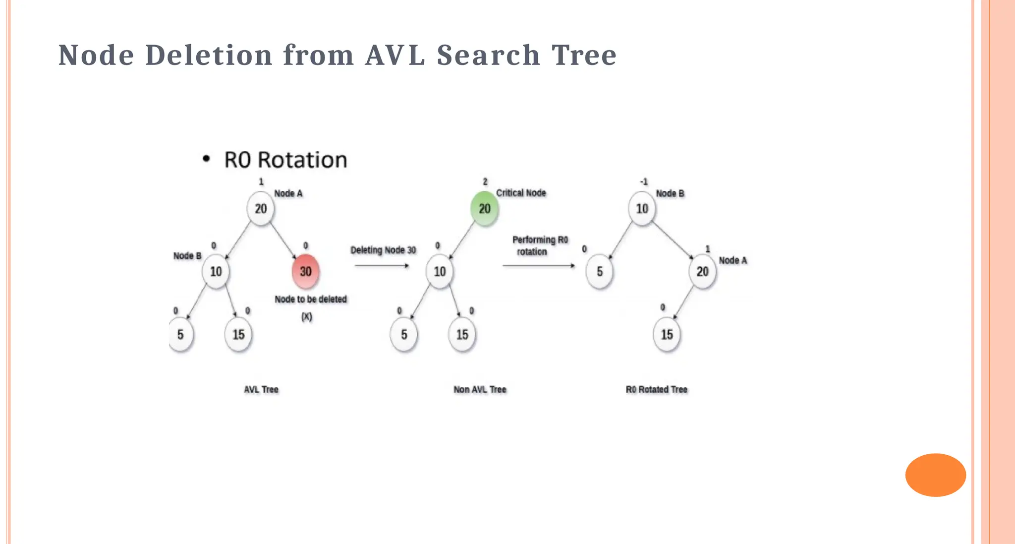
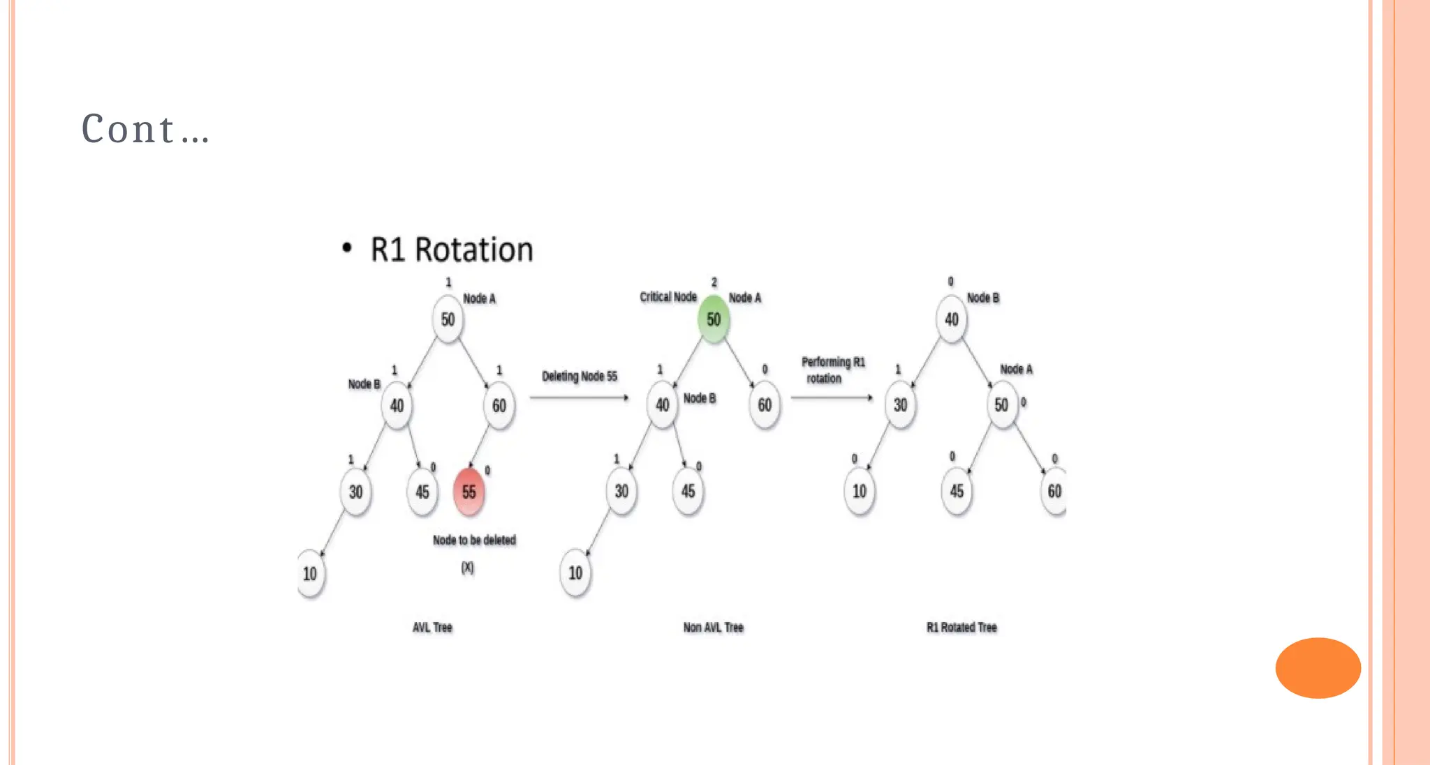
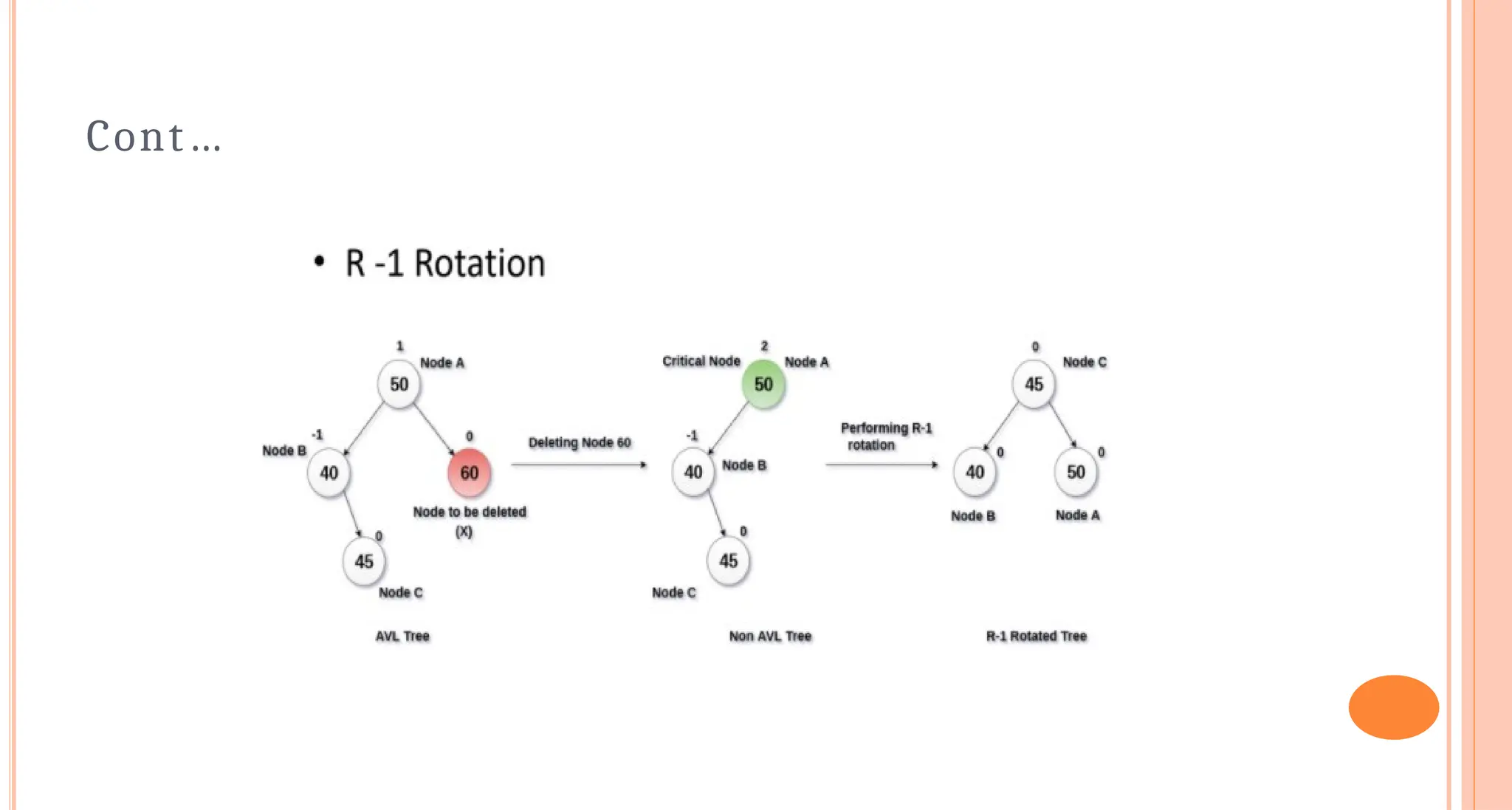
AVL Tree
An emptybinary tree is an AVL tree. A non empty binary tree is an AVL
tree iff given TL and TR to be the left and right subtrees of T and h(TL)
and h(TL) and h(TR) to be heights of subtrees TL and TR respectively. TL
and TR are AVL trees and |h(TL) - h(TR)| ≤ 1
h(TL) - h(TR) is known as the balance factor (BF) and for AVL tree, the
balance factor of a node can be either 0, 1 or -1.
An AVL search tree is a binary search tree which is an AVL tree.
49.
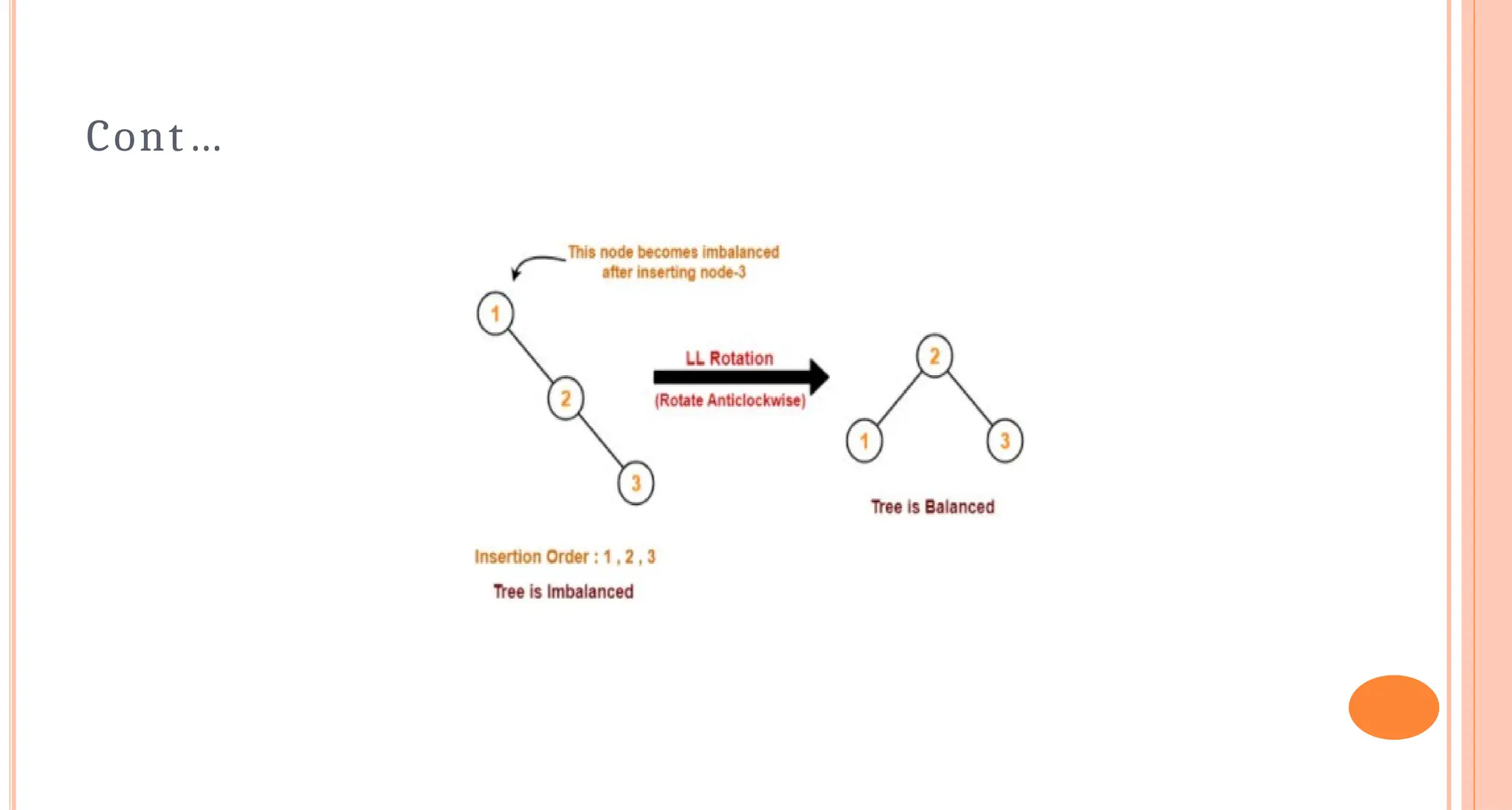
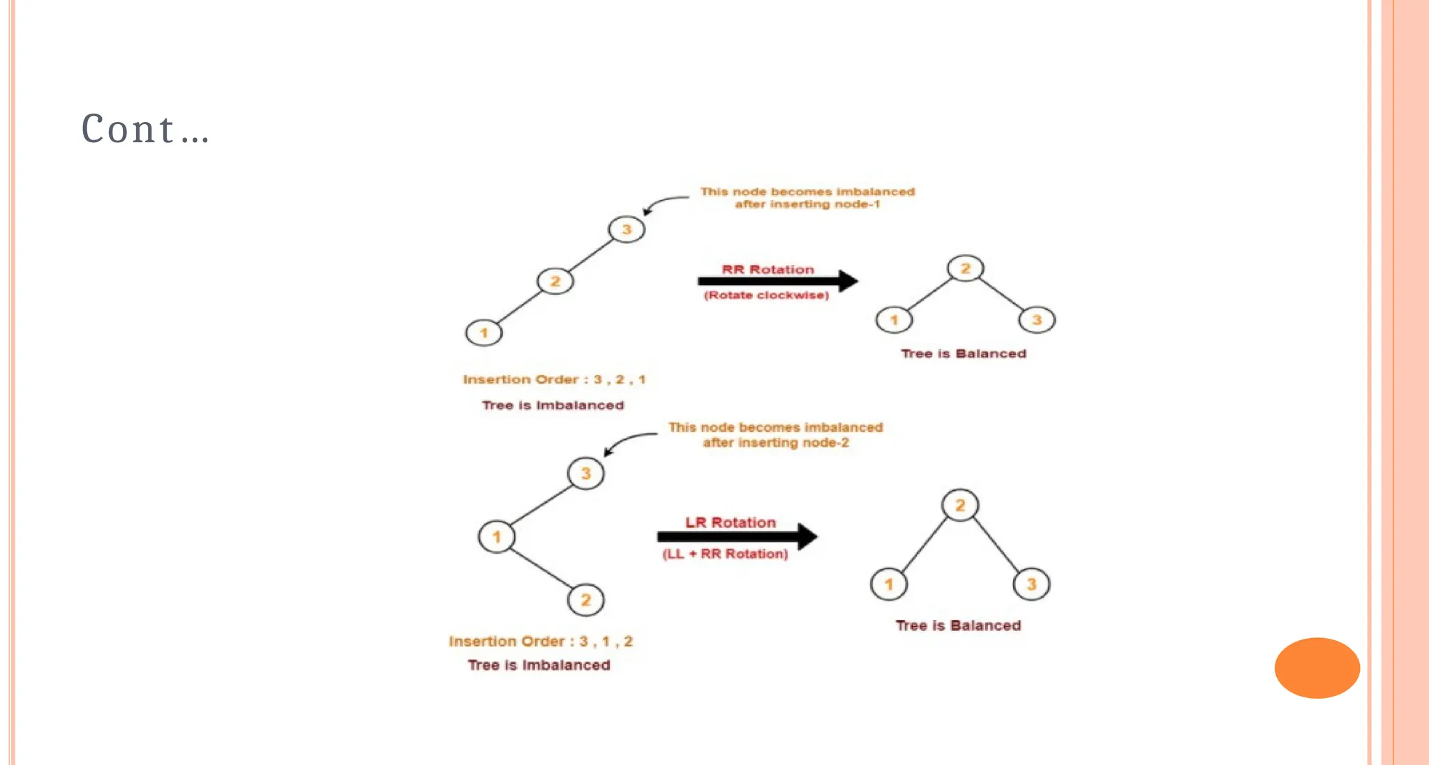
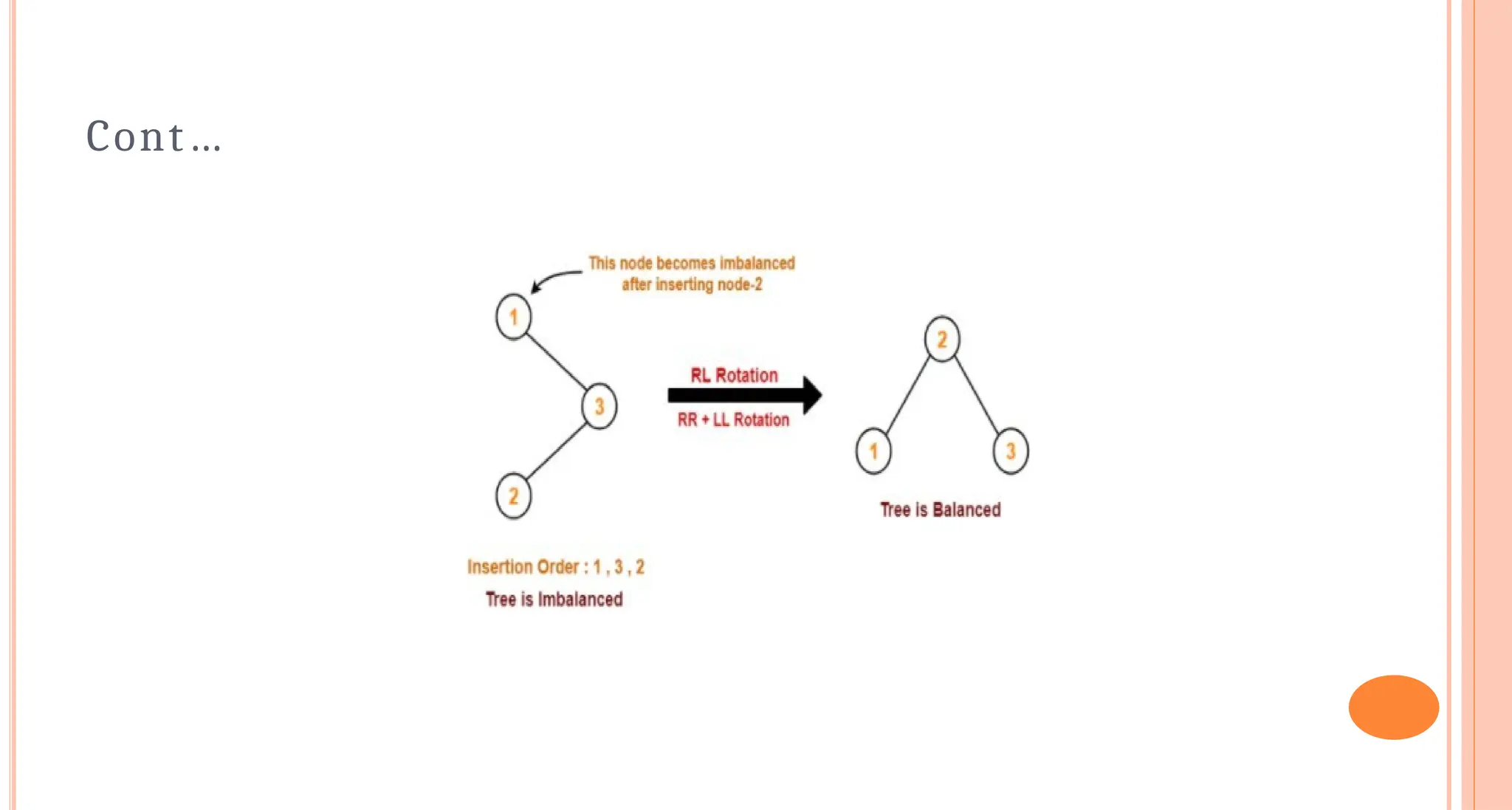
INSERTION in AVLSearch Tree
LL rotation: Inserted node is in the left subtree of left subtree of node A
RR rotation: Inserted node is in the right subtree of right subtree of node
A
LR rotation: Inserted node is in the right subtree of left subtree of node
A
RL rotation: Inserted node is in the left subtree of right subtree of node
A
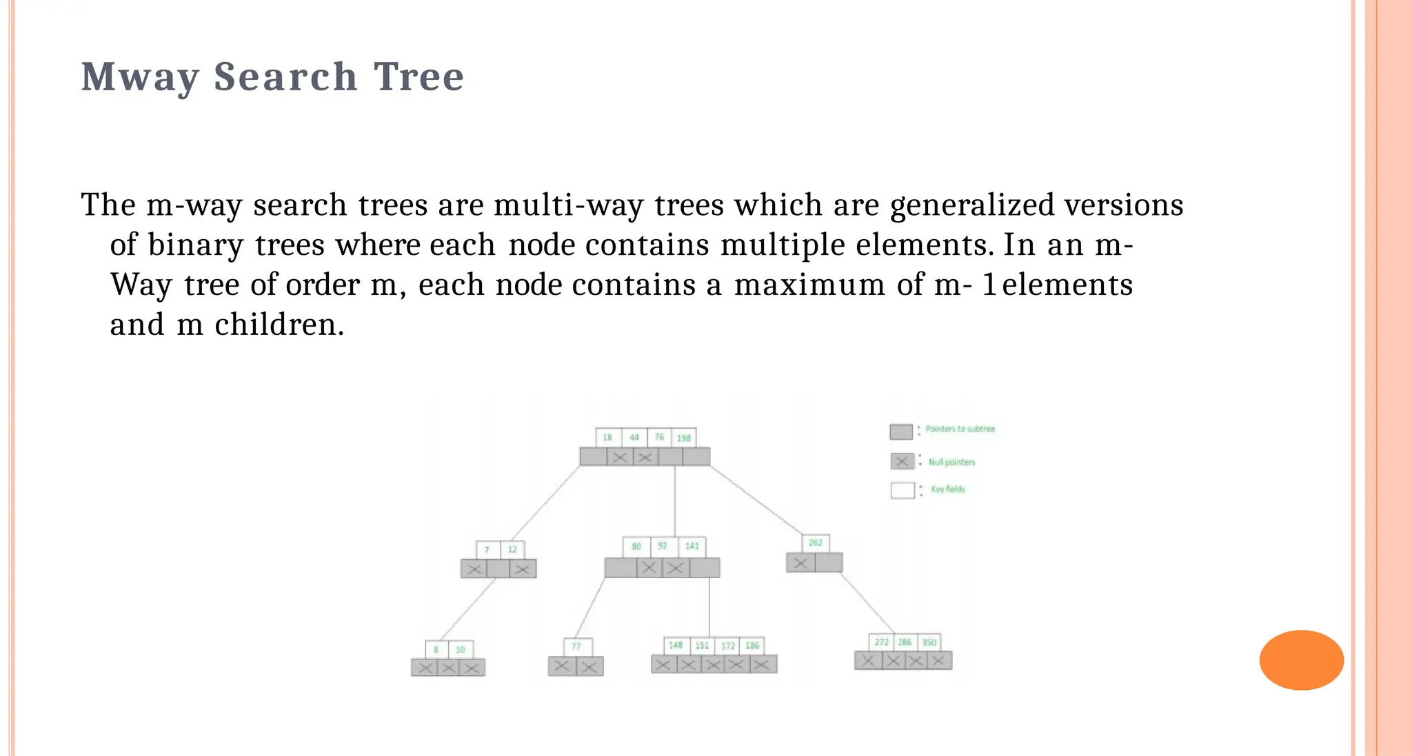
Mway Search Tree
Them-way search trees are multi-way trees which are generalized versions
of binary trees where each node contains multiple elements. In an m-
Way tree of order m, each node contains a maximum of m- 1 elements
and m children.
B Tree
Definition
A B-treeof order m, if non empty, is an m-way search tree in which:
(i) the root has at least two child nodes and at most m child nodes
(ii)the internal nodes except the root have at least [m/2] child nodes
and at most m child nodes.
(iii)the number of keys in each internal node is one less than the
number of child nodes and these keys partition the keys in the subtrees of
the node in a manner similar to that of m-way search trees.
(iv) all leaf nodes are on the same level.
59.
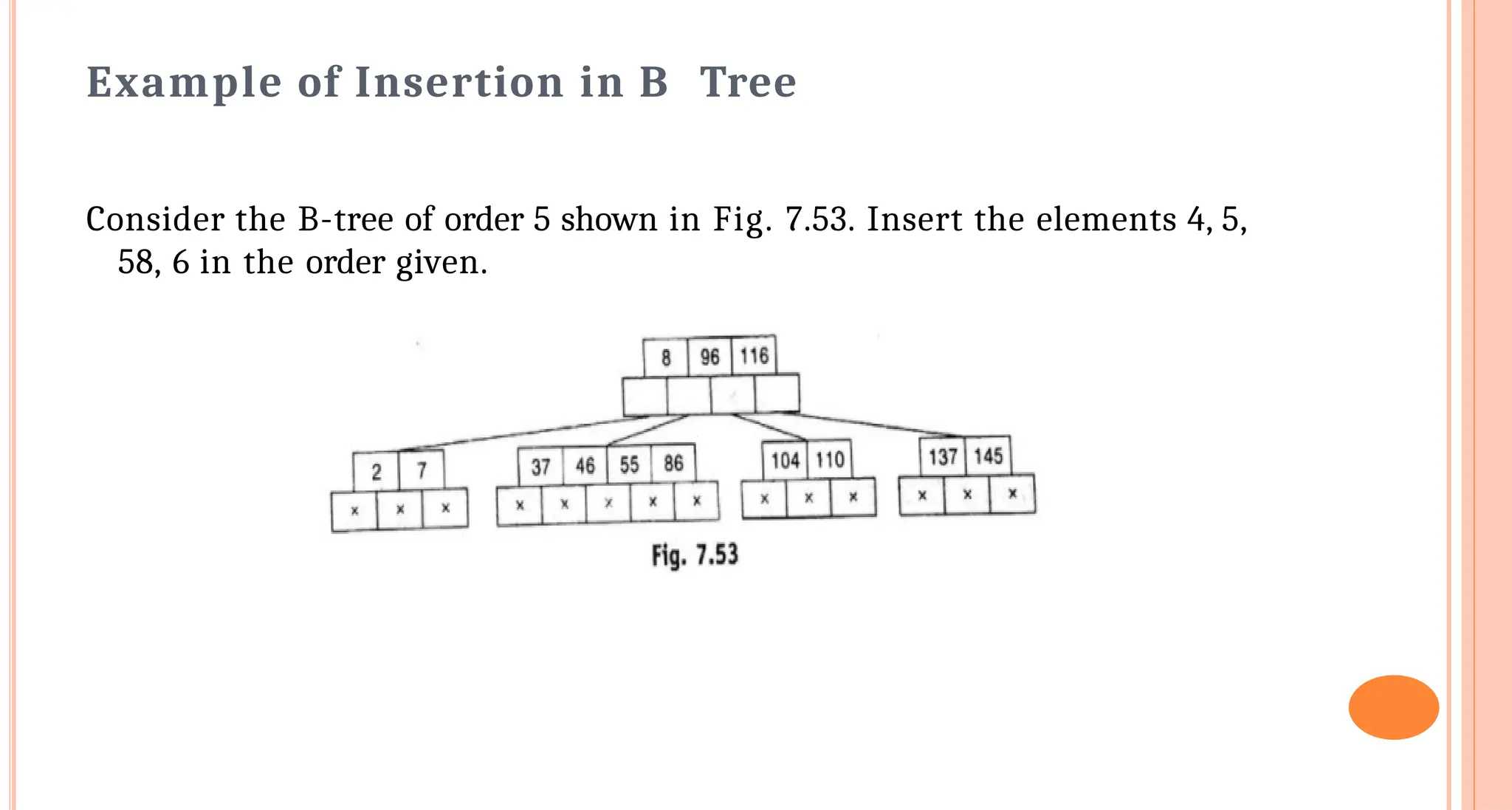
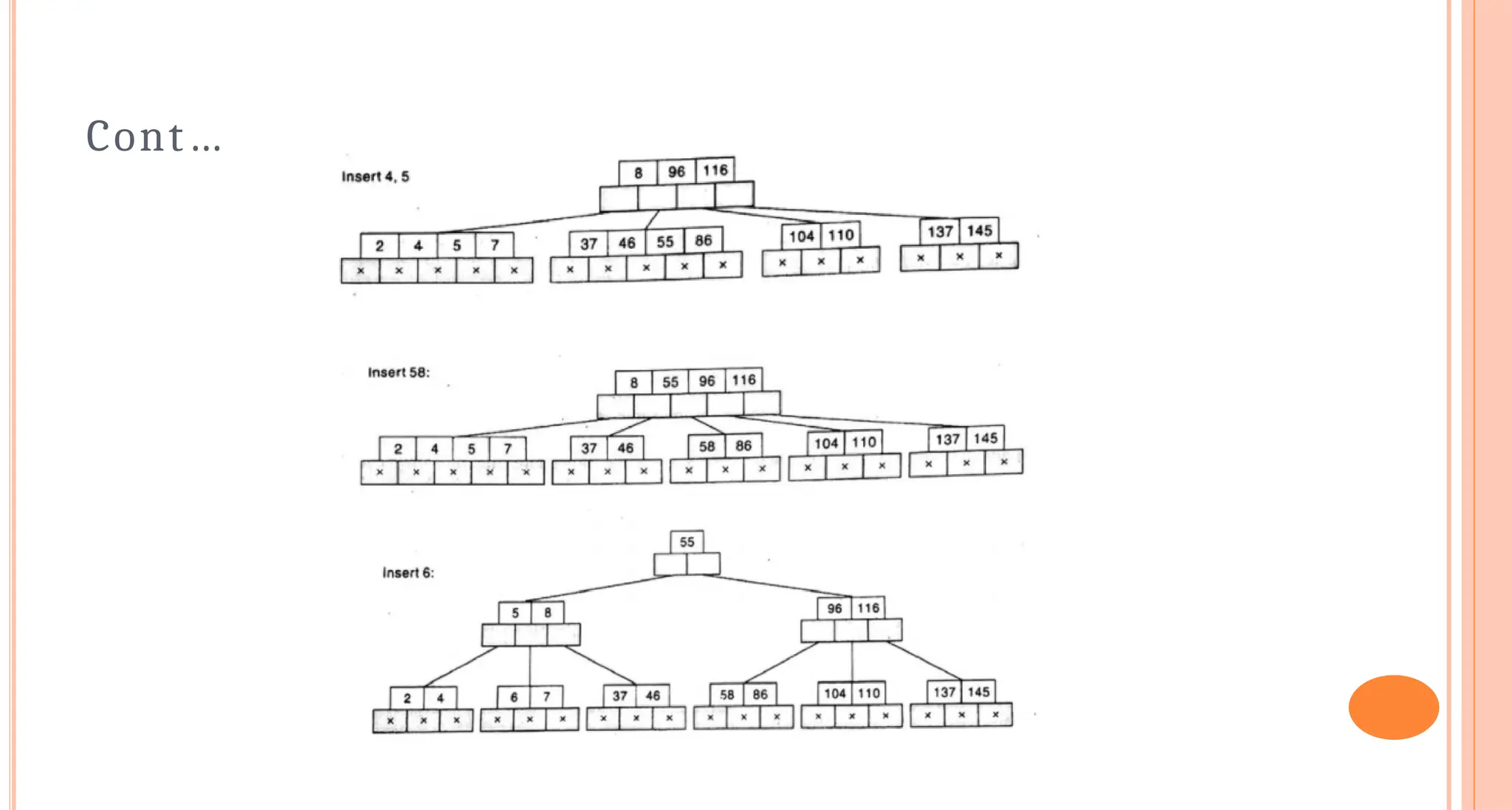
Example of Insertionin B Tree
Consider the B-tree of order 5 shown in Fig. 7.53. Insert the elements 4, 5,
58, 6 in the order given.
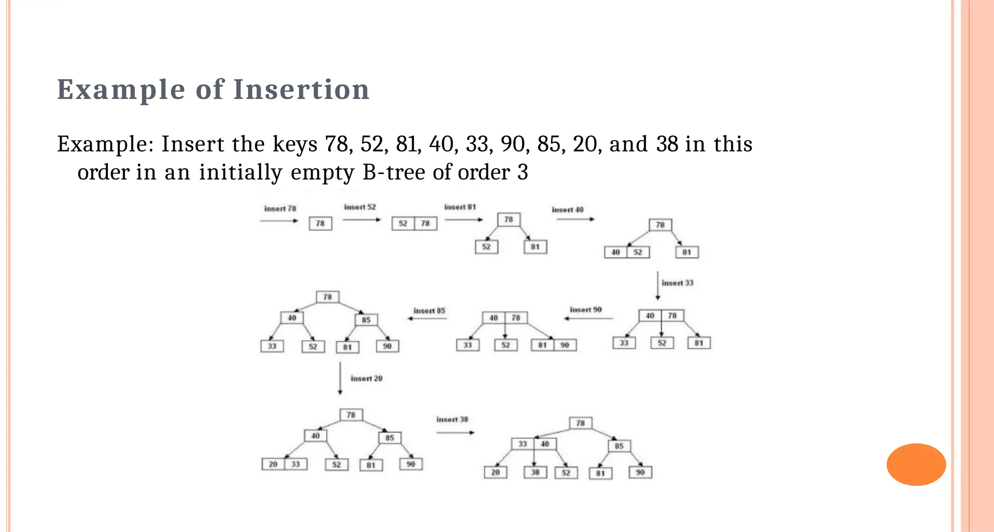
Example of Insertion
Example:Insert the keys 78, 52, 81, 40, 33, 90, 85, 20, and 38 in this
order in an initially empty B-tree of order 3
64.
Node Searching inBTree
Search Operation
The search operation is the simplest operation on B Tree.
The following algorithm is applied:
• Let the key (the value) to be searched by "k".
• Start searching from the root and recursively traverse
down.
•If k is lesser than the root value, search left subtree, if k is greater
than the root value, search the right subtree.
• If the node has the found k, simply return the node.
•If the k is not found in the node, traverse down to the child with a
greater key.
• If k is not found in the tree, we return NULL.
65.
Tournament Tree
Tournament treeis a complete binary tree n external nodes and n-1
internal nodes. The external nodes represent the players and internal
nodes represent the winner of the match between the two players.
Properties of Tournament Tree:
1.It is rooted tree i.e. the links in the tree and directed from parents
to children and there is a unique element with no parents.
2.Trees with a number of nodes not a power of 2 contain holes which
is general may be anywhere in the tree.
3. The tournament tree is also called selection tree.
4.The root of the tournament tree represents overall winner of the
tournament.
66.
Types of TournamentTree
There are mainly two type of tournament tree
1. Winner tree
2. Loser tree
67.
Cont…
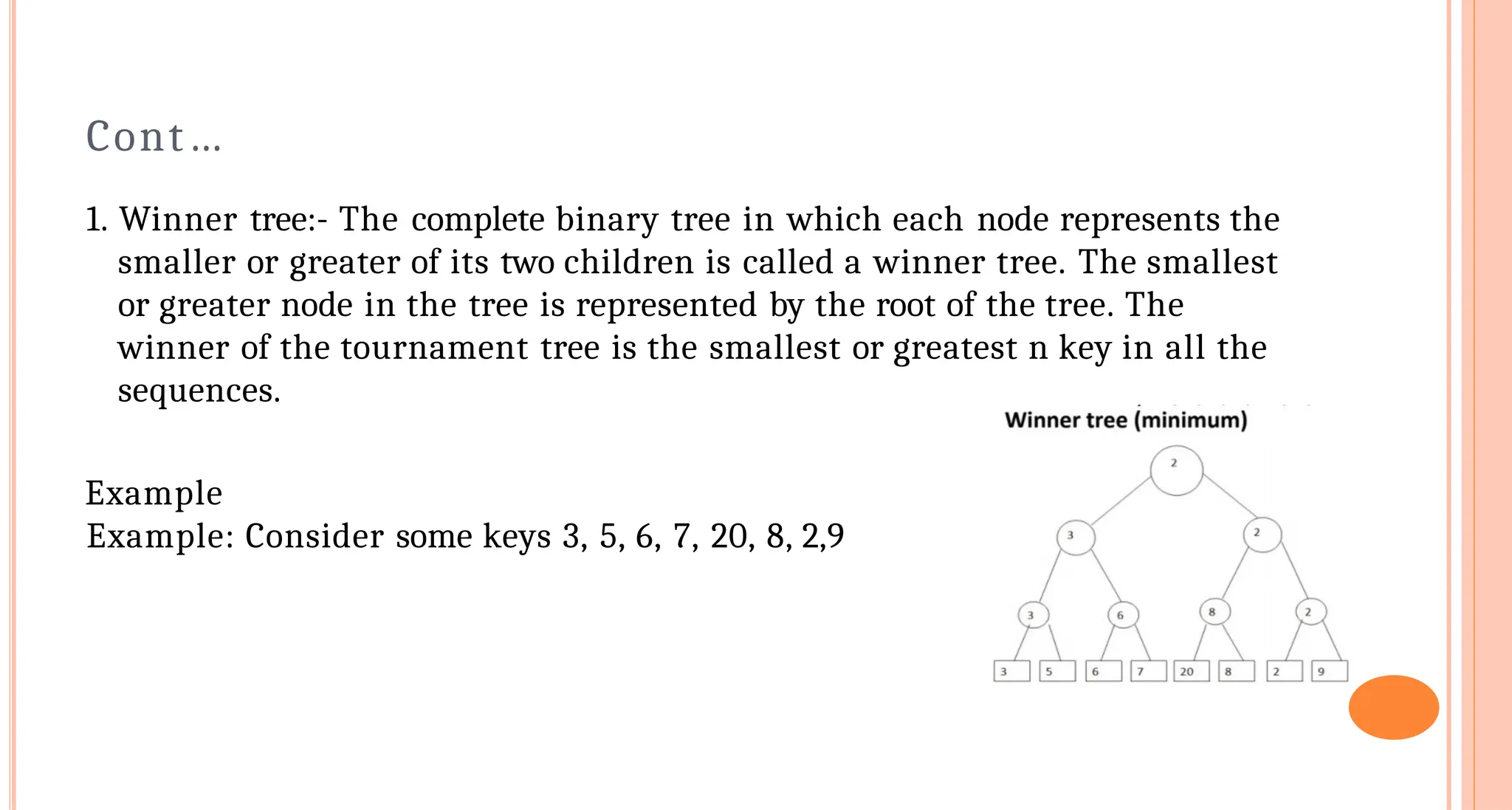
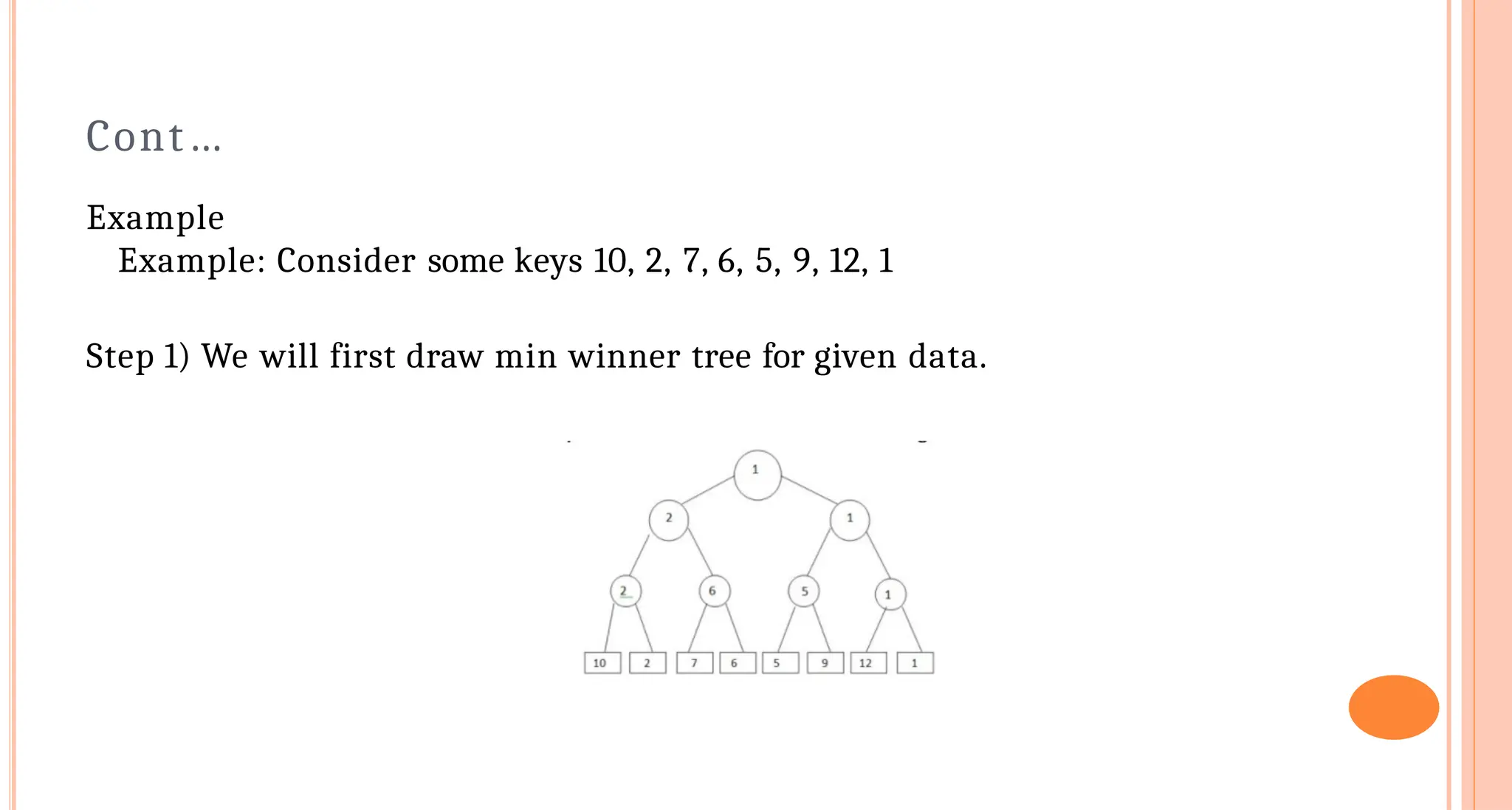
1. Winner tree:-The complete binary tree in which each node represents the
smaller or greater of its two children is called a winner tree. The smallest
or greater node in the tree is represented by the root of the tree. The
winner of the tournament tree is the smallest or greatest n key in all the
sequences.
Example
Example: Consider some keys 3, 5, 6, 7, 20, 8, 2,9
68.
Cont…
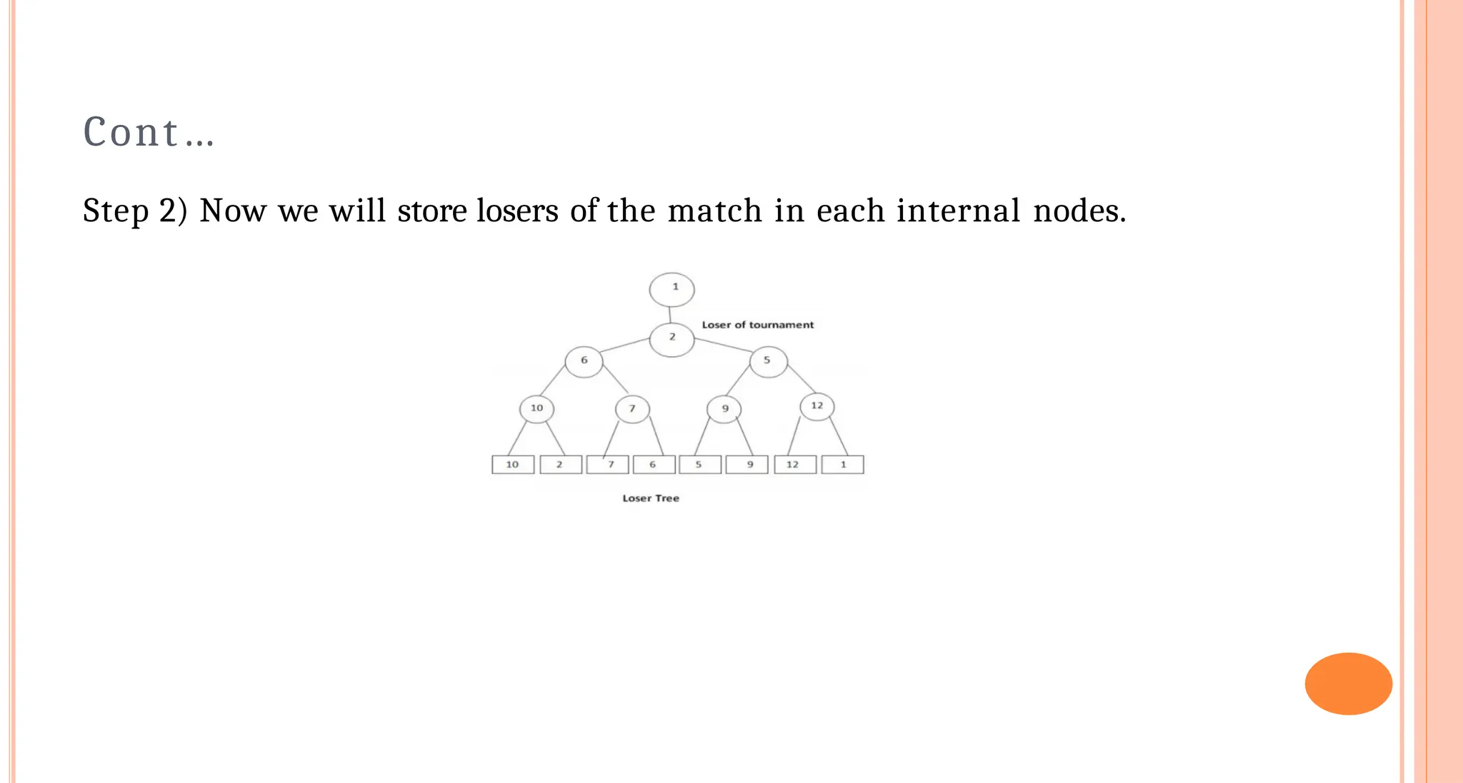
2. Loser Tree:-The complete binary tree for n players in which there are n
external nodes and n-1 internal nodes then the tree is called loser tree.
The loser of the match is stored in internal nodes of the tree. But in this
overall winner of the tournament is stored at tree [O]. The loser is an
alternative representation that stores the loser of a match at the
corresponding node. An advantage of the loser is that to restructure the
tree after a winner tree been output, it is sufficient to examine node on
the path from the leaf to the root rather than the sibling of nodes on this
path.
Cont…
Step 2) Nowwe will store losers of the match in each internal nodes.
71.
Data Structure :Graph
• A data structure that consists of a set of nodes (vertices) and a set of
edges that relate the nodes to each other.
• The set of edges describes relationshipsamong the vertices .
• A graph G is defined as
follows: G=(V,E)
V(G): a finite, nonempty set of vertices
E(G): a set of edges (pairs of vertices)
72.
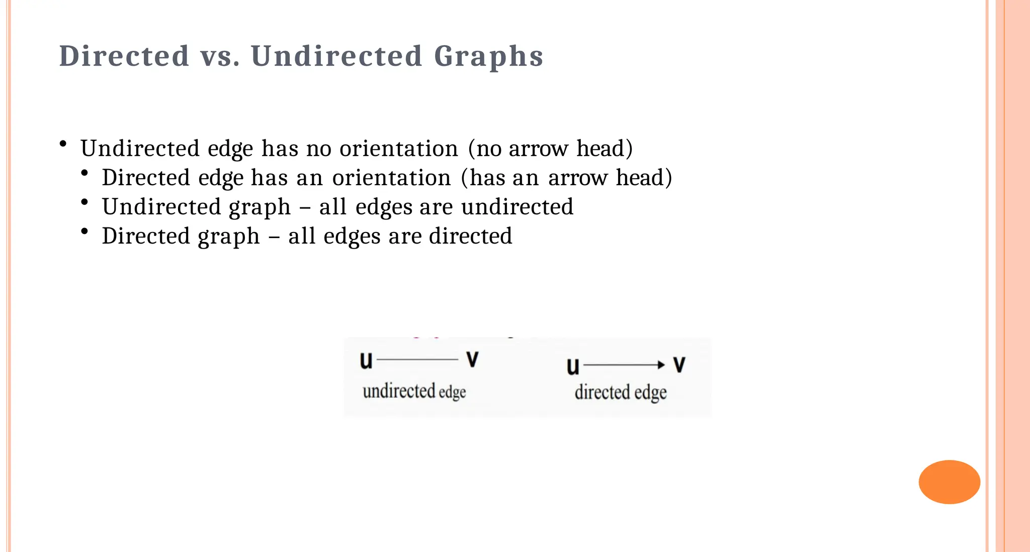
Directed vs. UndirectedGraphs
• Undirected edge has no orientation (no arrow head)
• Directed edge has an orientation (has an arrow head)
• Undirected graph – all edges are undirected
• Directed graph – all edges are directed
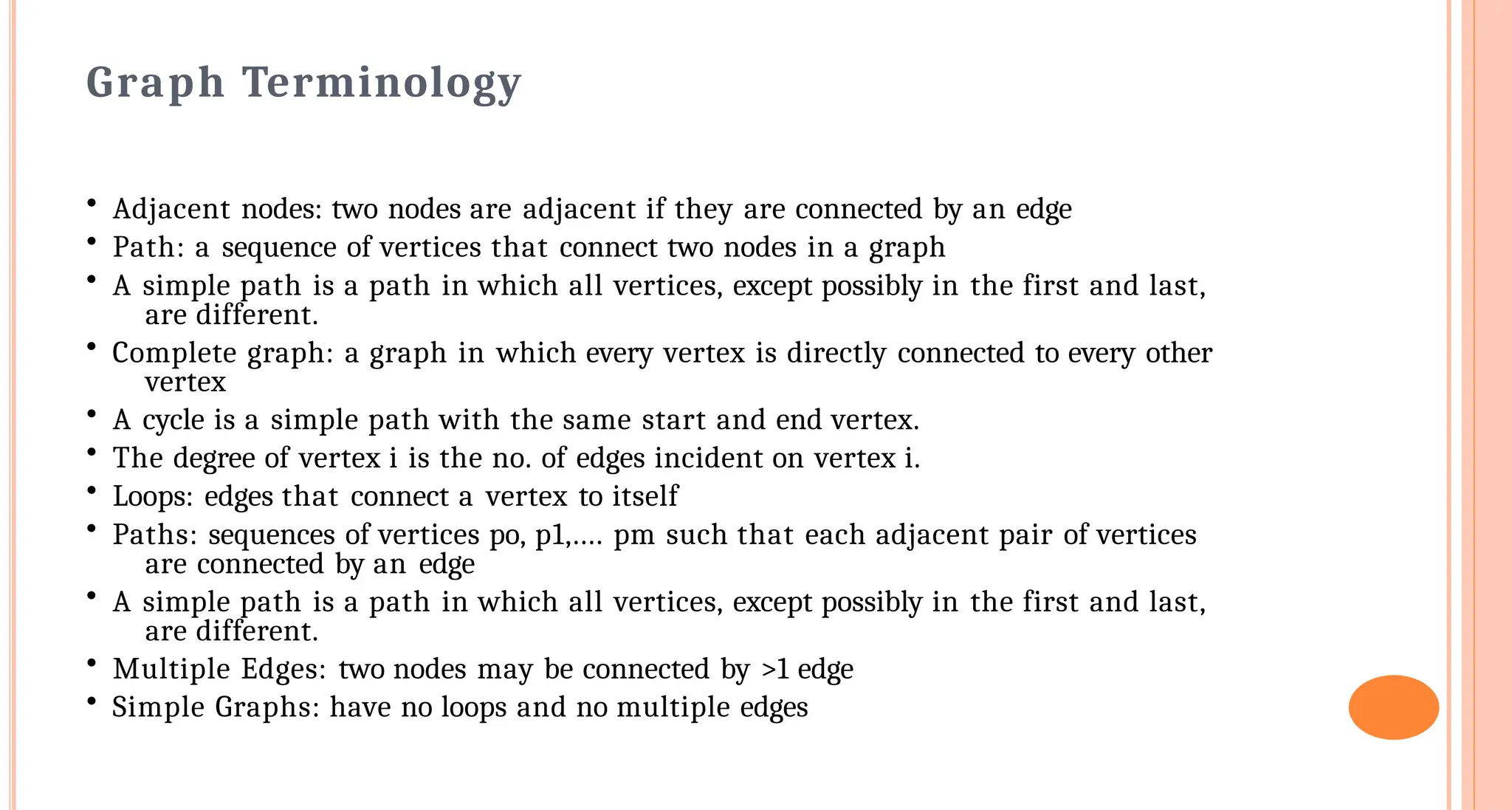
Graph Terminology
• Adjacentnodes: two nodes are adjacent if they are connected by an edge
• Path: a sequence of vertices that connect two nodes in a graph
• A simple path is a path in which all vertices, except possibly in the first and last,
are different.
• Complete graph: a graph in which every vertex is directly connected to every other
vertex
• A cycle is a simple path with the same start and end vertex.
• The degree of vertex i is the no. of edges incident on vertex i.
• Loops: edges that connect a vertex to itself
• Paths: sequences of vertices po, p1,.... pm such that each adjacent pair of vertices
are connected by an edge
• A simple path is a path in which all vertices, except possibly in the first and last,
are different.
• Multiple Edges: two nodes may be connected by >1 edge
• Simple Graphs: have no loops and no multiple edges
75.
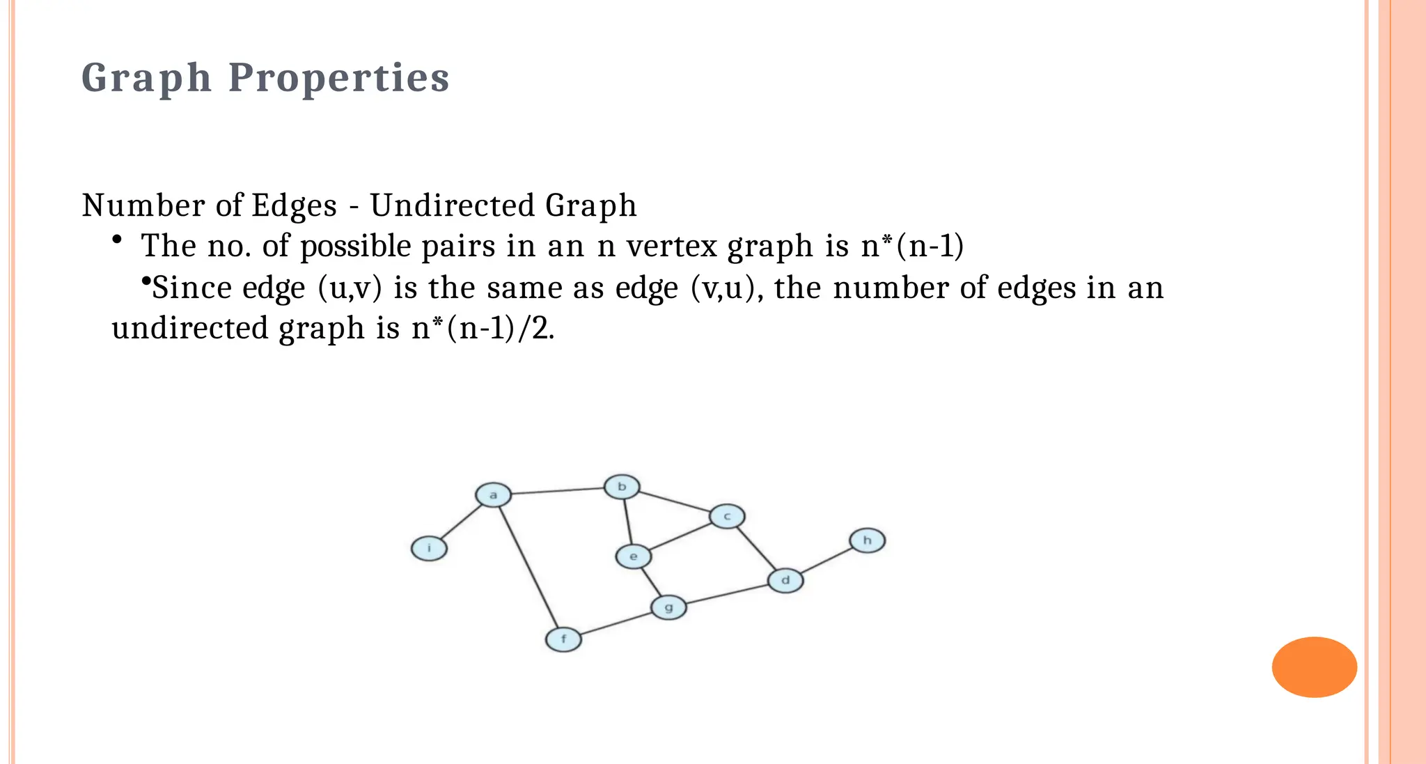
Graph Properties
Number ofEdges - Undirected Graph
• The no. of possible pairs in an n vertex graph is n*(n-1)
•Since edge (u,v) is the same as edge (v,u), the number of edges in an
undirected graph is n*(n-1)/2.
76.
Cont…
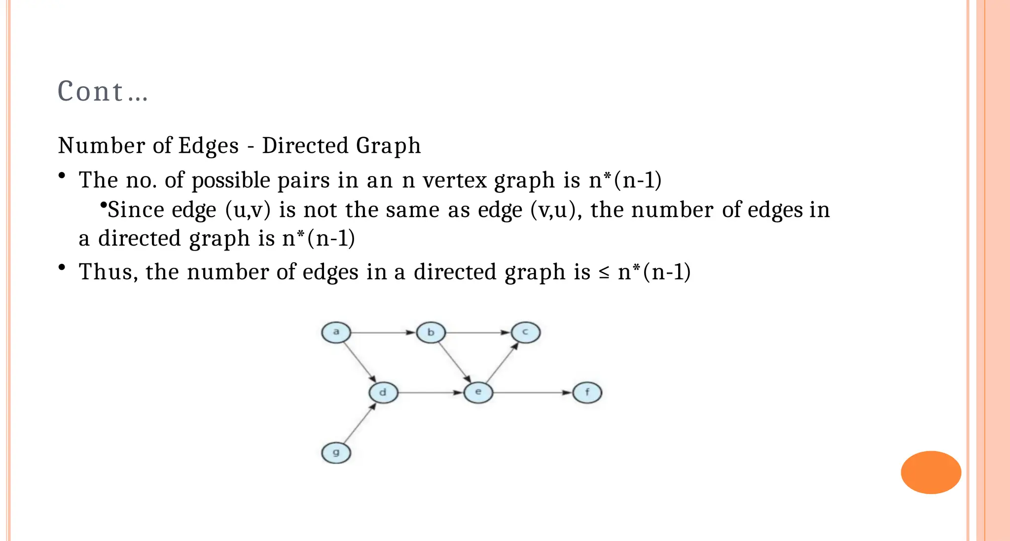
Number of Edges- Directed Graph
• The no. of possible pairs in an n vertex graph is n*(n-1)
•Since edge (u,v) is not the same as edge (v,u), the number of edges in
a directed graph is n*(n-1)
• Thus, the number of edges in a directed graph is ≤ n*(n-1)
77.
Cont…
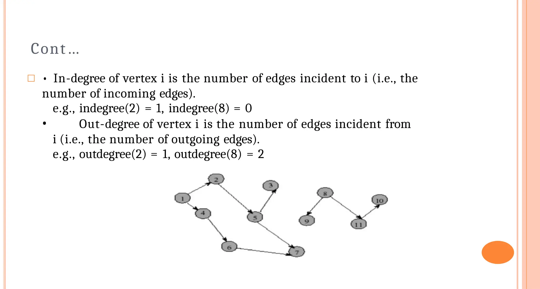
□ • In-degreeof vertex i is the number of edges incident to i (i.e., the
number of incoming edges).
e.g., indegree(2) = 1, indegree(8) = 0
• Out-degree of vertex i is the number of edges incident from
i (i.e., the number of outgoing edges).
e.g., outdegree(2) = 1, outdegree(8) = 2
78.
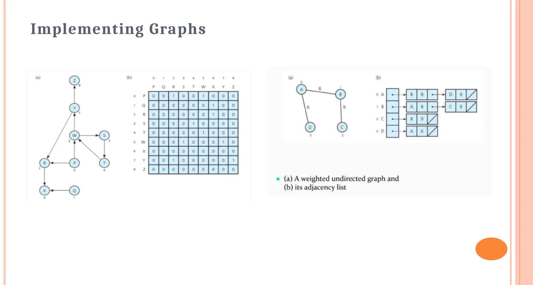
Graph Representation
• Forgraphs to be computationally useful, they have to be conveniently
represented in programs
• There are two computer representations of graphs:
• Adjacency matrix representation
• Adjacency lists representation
79.
Adjacency Matrix
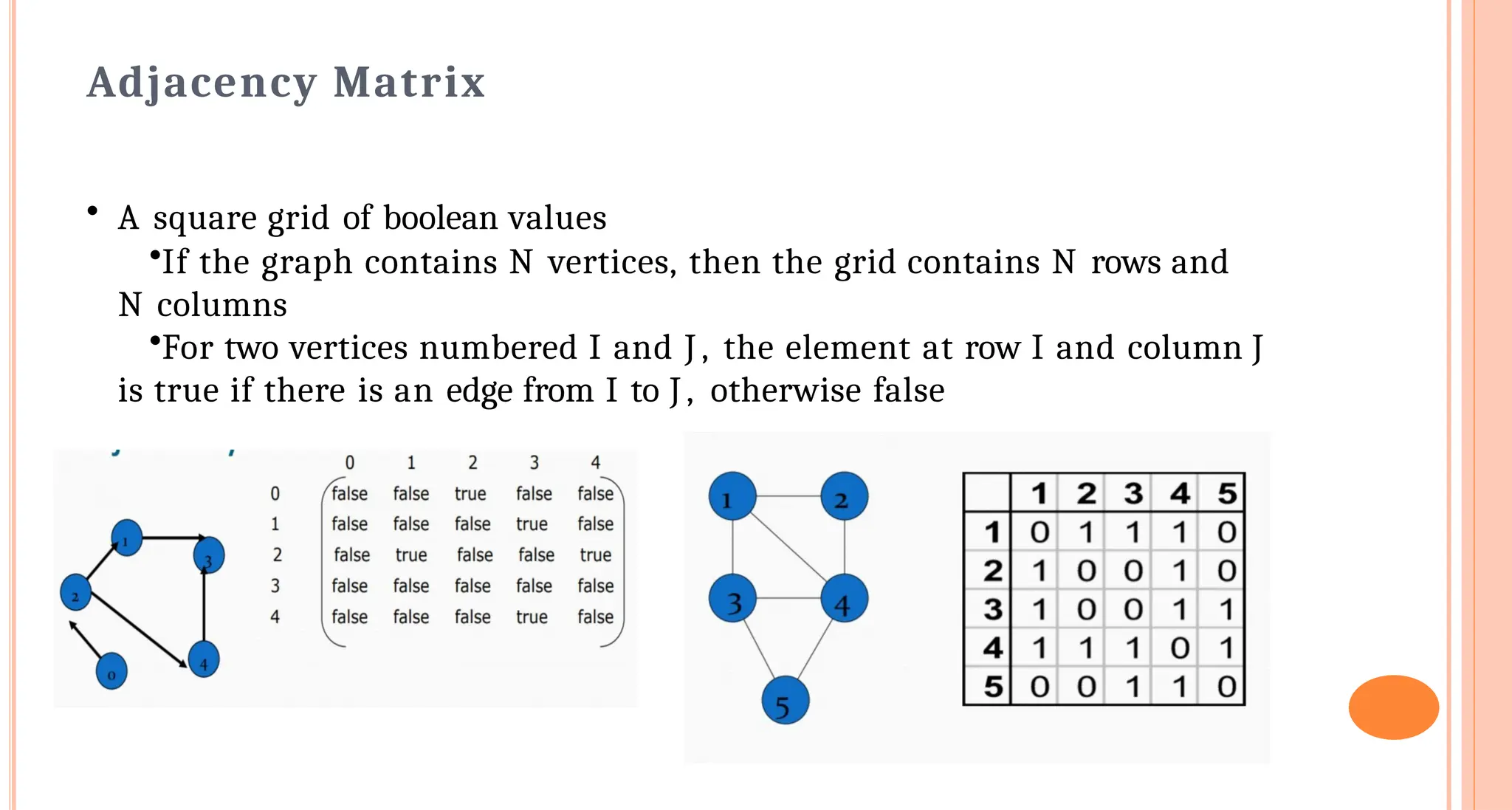
• Asquare grid of boolean values
•If the graph contains N vertices, then the grid contains N rows and
N columns
•For two vertices numbered I and J , the element at row I and column J
is true if there is an edge from I to J , otherwise false
80.
Adjacency Lists Representation
•A graph of n nodes is represented by a one- dimensional array L of
linked lists, where
• L[i] is the linked list containing all the nodes adjacent from node
i.
• The nodes in the list L[i] are in no particular order
![Memory Representation of Binary Tree
1. Array Representation of Binary Tree:-
(i)Root is stored in a[0]
(ii)Node occupies- a[i]
• Left child-[2*i+1]
• Right child-[2*i+2]
• Parent node-[(i-1)/2]](https://image.slidesharecdn.com/cs-245ppt-250918080107-f8272835/75/DATA-STRUCTURES-AND-ALGORITHMS-UNIT-1-pptx-35-2048.jpg)
![PREORD(INFO, LEFT, RIGHT, ROOT)
A binary tree T is in memory. The algorithm does a preorder traversal of T, applying an
operation PROCESS to each of its nodes. An array STACK is used to temporarily hold
the addresses of nodes.
1. [Initially push NULL onto STACK, and initialize PTR.]
Set TOP := 1, STACK[1] := NULL and PTR := ROOT.
2. Repeat Steps 3 to 5 while PTR = NULL:
3. Apply PROCESS to INFO[PTR].
4. [Right child?]
If RIGHT[PTR] = NULL, then: [Push on STACK.]
Set TOP := TOP + 1, and STACK[TOP] := RIGHT[PTR].
[End of If structure.]
5.[Left child?]
If LEFT[PTR] NULL, then:
Set PTR := LEFT[PTR].
Else: [Pop from STACK.]
Set PTR := STACK[TOP]
and TOP := TOP - 1.
[End of If structure.]
[End of Step 2 loop.]
6. Exit.](https://image.slidesharecdn.com/cs-245ppt-250918080107-f8272835/75/DATA-STRUCTURES-AND-ALGORITHMS-UNIT-1-pptx-39-2048.jpg)
![INORD(INFO, LEFT, RIGHT, ROOT)
A binary tree is in memory. This algorithm does an inorder traversal of T, applying an operation
PROCESS to each of its nodes. An array STACK is used to temporarily hold the addresses of
nodes.
1. [Push NULL onto STACK and initialize PTR.]
Set TOP := 1, STACK[1] NULL and PTR := ROOT.
2. Repeat while PTR = NULL: (Pushes left-most path onto STACK.]
(a) Set TOP := TOP + 1 and STACK[TOP] := PTR. [Saves node.]
(b) Set PTR := LEFT[PTR). [Updates PTR.]
[End of loop.]
3. Şet PTR := STACK[TOP] and TOP := TOP - 1. [Pops node from
STACK.]
4. Repeat Steps 5 to 7 while PTR = NULL: [Backtracking.]
5. Apply PROCESS to INFO[PTR].
6. [Right child?] If RIGHT[PTR] # NULL, then:
(a) Set PTR := RIGH[PTR].
(b)Go to Step 2
[End of If structure.]
7. Set PTR :=
STACK[TOP] and
TOP := TOP -1. [Pops
node.]
[End of Step 4 loop.]
8. Exit.](https://image.slidesharecdn.com/cs-245ppt-250918080107-f8272835/75/DATA-STRUCTURES-AND-ALGORITHMS-UNIT-1-pptx-40-2048.jpg)
![POSTORD(INFO, LEFT, RIGHT, ROOT)
A binary tree T is in memory. This algorithm does a postorder traversal of T. applying an operation PROCESS to each
of its nodes. An array STACK is used to temporarily hold the addresses of nodes.
1. [Push NULL onto STACK and initialize PTR.]
Set TOP := 1. STACK[1] := NULL and PTR := ROOT.
2. [Push left-most path onto STACK]
Repeat Steps 3 to 5 while PTR
NULL:
3. Set TOP := TOP + 1 and
STACK[TOP] := PTR.
[Pushes PTR on STACK]
4. If RIGHT[PTR] NULL, then: [Push on
STACK.]
Set TOP := TOP + 1 and
STACK[TOP] := -RIGHT[PTR].
[End of If structure.)
5. Set PTR := LEFT[PTR]. [Updates pointer PTR.]
[End of Step 2 loop.)
6. Set PTR := STACK[TOP] and TOP := TOP - 1.
[Pops node from STACK.]
7. Repeat while PTR > 0:
(a) Apply PROCESS to INFO[PTR).
(b) Set PTR := STACK[TOP] and TOP := TOP - 1.
[Pops node from STACK.]
[End of loop.]
8. If PTR <0, then:](https://image.slidesharecdn.com/cs-245ppt-250918080107-f8272835/75/DATA-STRUCTURES-AND-ALGORITHMS-UNIT-1-pptx-41-2048.jpg)
![Algo. For Location Finding
FIND(INFO, LEFT. RIGHT, ROOT. ITEM, LOC, PAR)
A binary search tree T is in memory and an ITEM of information is given. This procedure finds the location LOC of
ITEM in T and also the location PAR of the parent of ITEM. There are three special cases:
(i) LOC = NULL and PAR - NULL will indicate that the tree is empty.
(ii) LOC NULL and PAR - NULL will indicate that ITEM is the root of T.
(iii) LOC = NULL and PAR = NULL will indicate that ITEM is not in T and can be added to T as a child of the node N
with location PAR.
1. [Tree empty?]
If ROOT = NULL, then: Set LOC := NULL and PAR := NULL. And Return.
2. [ITEM at root?]
If ITEM - INFO[ROO]), then: Set LOC := ROOT and PAR = NULL, and Return.
3. [Initialize pointers PTR and SAVE.]
If ITEM <INFO[ROOT]), then:
Set PTR := LEFT[ROOT] and SAVE := ROOT.
Else:
Set PTR := RIGHT[ROOT] and SAVE := ROOT
[End of If structure.]
4. Repeat Steps 5 and 6 while PTR ≠ NULL.
5. [ITEM found?]
If ITEM = INFO[PTR], then: Set LOC := PTR and PAR := SAVE and Return.
6. IF ITEM < INFO[PTR], then:
Set SAVE := PTR and PTR := LEFT[PTR].
Else:
Set SAVE := PTR and PTR := RIGHT[PTR].
[End of If structure.]
[End of Step 4 loop.]
7. [Search unsuccessful.] Set LOC:= NULL and PAR := SAVE.
8. Exit.](https://image.slidesharecdn.com/cs-245ppt-250918080107-f8272835/75/DATA-STRUCTURES-AND-ALGORITHMS-UNIT-1-pptx-45-2048.jpg)
![Insertion Algo. For BST
INSBST(INFO, LEFT, RIGHT, ROOT, AVAIL, ITEM, LOC)
A binary search tree T is in memory and an ITEM of information is given. This algorithm finds the
location LOC of ITEM in T or adds ITEM as a new node in T at location LOC.
1. Call FIND(INFO, LEFT, RIGHT, ROOT, ITEM, LOC, PAR).
[Procedure 7.4.)
2. If LOC ≠ NULL, then Exit.
3. [Copy ITEM into new node in AVAIL list.]
(a) IF AVAIL = NULL, then: Write: OVERFLOW, and Exit.
(b) Set NEW = AVAIL, AVAIL :=
LEFT[AVAIL] and INFO[NEW] := ITEM.
(c) Set LOC := NEW. LEFT[NEW] := NULL and
RIGHT[NEW] := NULL.
4. [Add ITEM to tree.]
If PAR = NULL, then:
Set ROOT := NEW.
Else if ITEM < INFO[PAR], then:
Set LEFT[PAR] := NEW.
Else:
Set RIGHT[PAR] := NEW.
[End of If structure.]
5. Exit.](https://image.slidesharecdn.com/cs-245ppt-250918080107-f8272835/75/DATA-STRUCTURES-AND-ALGORITHMS-UNIT-1-pptx-46-2048.jpg)
![B Tree
Definition
A B-tree of order m, if non empty, is an m-way search tree in which:
(i) the root has at least two child nodes and at most m child nodes
(ii)the internal nodes except the root have at least [m/2] child nodes
and at most m child nodes.
(iii)the number of keys in each internal node is one less than the
number of child nodes and these keys partition the keys in the subtrees of
the node in a manner similar to that of m-way search trees.
(iv) all leaf nodes are on the same level.](https://image.slidesharecdn.com/cs-245ppt-250918080107-f8272835/75/DATA-STRUCTURES-AND-ALGORITHMS-UNIT-1-pptx-58-2048.jpg)
![Cont…
2. Loser Tree:- The complete binary tree for n players in which there are n
external nodes and n-1 internal nodes then the tree is called loser tree.
The loser of the match is stored in internal nodes of the tree. But in this
overall winner of the tournament is stored at tree [O]. The loser is an
alternative representation that stores the loser of a match at the
corresponding node. An advantage of the loser is that to restructure the
tree after a winner tree been output, it is sufficient to examine node on
the path from the leaf to the root rather than the sibling of nodes on this
path.](https://image.slidesharecdn.com/cs-245ppt-250918080107-f8272835/75/DATA-STRUCTURES-AND-ALGORITHMS-UNIT-1-pptx-68-2048.jpg)
![Adjacency Lists Representation
• A graph of n nodes is represented by a one- dimensional array L of
linked lists, where
• L[i] is the linked list containing all the nodes adjacent from node
i.
• The nodes in the list L[i] are in no particular order](https://image.slidesharecdn.com/cs-245ppt-250918080107-f8272835/75/DATA-STRUCTURES-AND-ALGORITHMS-UNIT-1-pptx-80-2048.jpg)