The provincial, City or Municipality Assessor shall undertake of real property assessment once every three (3) years, which shall commence upon the enacment of the Schedule of Fair Market Values (SFMV) into an ordinance by the sanggunian concerned.
GENERAL REVISION OFREAL
PROPERTY ASSESSMENT AND
PREPARATION OF THE
SCHEDULE OF MARKET VALUES
2.
• The provincial,City or Municipality Assessor
shall undertake of real property assessment
once every three (3) years, which shall
commence upon the enacment of the
Schedule of Fair Market Values (SFMV) into an
ordinance by the sanggunian concerned.
3.
• For thispurpose, the Provicial Assessors, the City
Assessors and the Municipal Assessor of the
Metropolitan Manila Area shall prepare the
Schedude of Fair Market Values for the different
kinds and classes of real property within the
teritorial jurisdiction of the province, city or
municipality in accordance with the Dept. Of
Finance, Bureau of Local Goverment Finance,
Manual on Real Property Appraisal and Assessment
Operation.
4.
• In thecase of the Metro Manila Area, the assessor of
each assessment district shall meet and discuss and
hamonize their respective Schedule of Fair Market
Values.
• However, if there is no sufficient time or resources to
complete the work for all real property unit (RPUs)
with in the territorial jurisdiction of a particular local
government unit, a partial revision may be
undertaken by kind or class of real property
5.
For example:
• ByKind
– 1st year- All Lands
– 2nd year- All other real properties
• By Class
– 1st year- All Commercial and Industrial Properties
– 2nd year- All Other Classes of Properties
6.
• Purpose ofthe General Revision of Real
Property Assessments
– Equalizing and Updating valuations
• Rediscovery of real properties that have been “LOST”
from the tax rolls.
• Enables the assessor to purge the rolls of the double
assessment of properties that have accumulated
through the years.
7.
Appraisal/Assessment Calendar
• Forthe purpose of the general revision of real
property assessments the appraisal and
assessment process and its components
activity shall be governed by the calendar here
in prescribe as follows:
8.
ACTIVITY LGU Official(s)
RESPONSIBLE
PERIOD
Acceptanceof sworn
statements declaring the
true values of real property
to be filled by real property
owners/administrators.
The Provincial and City
Assessor and Municipal
Assessors of the
municipalities within Metro
Manila Area.
January 1 to June 30 of the
first year.
Analysis of data have been
gathered and preparation
of the preliminary
Schedule of Fair Market
Values.
The Provincial and City
Assessor and Municipal
Assessors of the
municipalities within Metro
Manila Area.
July 1 to September 30 of
the first year.
Preparation of final
Schedule of Fair Market
Values.
The Provincial and City
Assessor and Municipal
Assessors of the
municipalities within Metro
Manila.
Not later than October 15
of the first year.
9.
ACTIVITY LGU Official(s)
RESPONSIBLE
PERIOD
Submissionof the Schedule
of Fair Market Values to
the Sanggunian concerned
and conduct public
hearings.
The Provincial and City
Assessor and Municipal
Assessors of the
municipalities within Metro
Manila Area.
Not later than October 30
of the first year.
Enactment of Ordinace
adopting Schedule of Fair
Market Values.
The Sangguniang
Panlalawigan or
Panglungsod or
Sangguniang Bayan
concerned
Not later than January 31
of the second year.
Publication of the
Schedules in a newspaper
of general circulation in the
locality or posting in the
provincial Capitol, City or
Municipal Hall and in to
other conspicuous public
places
The Provincial and City
Assessor and Municipal
Assessors of the
municipalities within Metro
Manila.
Not later than February 28
of the second year.
10.
ACTIVITY LGU Official(s)
RESPONSIBLE
PERIOD
Preparationof Field
Appraisal and Assessment
Sheet, Tax Declaration and
Notice of Assessment and
mailing or delivering of said
notice to property owners.
The Provincial and City
Assessor and Municipal
Assessors of the
municipalities within Metro
Manila Area.
Not later than September
31 of the second year.
Prepartiong of Assessment
roles and the copies
thereof sent to Provincial,
City and Municipal
Treasurers.
The Provincial and City
Assessor and Municipal
Assessors of the
municipalities within Metro
Manila Area.
Not later than November
30 of the second year.
Effectivity of the Revised
Real Property Assessment
Provincial, City or
Municipal Assessors
Not later than January 1st
of the third year.
PREPARATION OF SMVBY
LOCAL ASSESSORS
Before any general revision of property
assessment is made pursuant to the provisions of
this Title (Title Two, Book II), there shall be a
prepared Schedule of Fair Market Values by the
provincial, city and municipal assessors of the
municipalities within MMA for the different classes
of real property situated in the respective LGUs for
enactment by ordinance by the sanggunian
concerned. x x x
(Sec 212, RA 7160)
13.
REVIEW OF SMVBY DOF-BLGF
The SMV, together with an abstract of the data
on which it is based, shall be submitted to the
BLGF Regional Offices concerned for review to
determine whether it conforms with the
provisions of the Local Government Code (LGC)
and the Local Assessment Regulations (LARs)
issued by the DOF not later than the 30th
day of
September of the 1st
year of the General Revision
Calendar prior to submission to the Sanggunian
concerned not later than October 30 of the same
year for enactment of an Ordinance.
14.
The SMV
• Providesthe matrix and other parameters
used in the appraisal and assessment of real
properties for taxation purposes
• Contains lists of locations (mostly roads, and
streets) setting out the unit base market
value (UBMV) and its classifications
15.
The SMV
• Setsadjustment factors (e.g., corner influence,
frontage, depth, location or proximity factors)
as basis to calculate individual land values
efficiently
• Includes the schedule of base unit construction
cost (SBUCC) for buildings and other
improvements
• Also includes the development of a
Depreciation Table adoptable to the locality
16.
SMV: BASIS OFAPPRAISAL FOR
TAXATION PURPOSES
The appraisal of real property shall be
based on the latest Schedule of Fair Market
Values (SFMV) prepared by the provincial,
city or municipal assessor within the MMA,
as embodied in an Ordinance passed by the
Sanggunian concerned.
17.
SMV: STANDARD FORMSAND
FORMATS
a) Letter of Transmittal
b) GR Form 1. Office Order/Schedule of Base Unit
Market Values for Residential, Commercial and
Industrial Land including Land Value Map
c) GR Form 2. Criteria for Sub-Classifica-tion of
Urban Lands
18.
d) GR Form3. Statement of Sales Value of
Residential, Commercial and Industrial Lands
e) GR Form 4. Tabulation of Sales Value for
each class of Residential, Commercial, and
Industrial Lands
f) GR Form 5. Computation for the Unit Base
Market Value of Urban Land
SMV: STANDARD FORMS AND
FORMATS
19.
g) GR Form6. Schedule of Market Value for
Agricultural Lands
h) GR Form 7. Statement of Sales Value of
Agricultural Land (if available
i) GR Form 8. Tabulation of Sales Values for
Agricultural Lands
SMV: STANDARD FORMS AND
FORMATS
20.
j) GR Form9. Computation for the Unit Base
Market Value Agricultural Lands
k) GR Form 10. Schedule of Base Unit
Construction Cost for Building (including
classification of building/ structures and
type of construction)
SMV: STANDARD FORMS AND
FORMATS
21.
l) GR Form11. Schedule of Depreciation
m) GR Form 12. Schedule of Unit Cost for
Extra Items
n) Computation for Unit Costs of Buildings
o) Miscellaneous Provision
SMV: STANDARD FORMS AND
FORMATS
MASS APPRAISAL:
Mass appraisalis the process of valuing multiple
properties as of a given date by systematic and
uniform application of appraisal methods and
techniques employing common data that allow for
statistical review and analysis of results.
24.
• Mass appraisalis the task of valuing many properties at the
same time.
• The difference between mass appraisal and individual appraisal
is in the manner in which the analyzed information is applied to
achieve the end result.
• Mass appraisal creates value estimates quickly, at the one date,
and at relatively low cost.
• Mass appraisal can address the question of uniformity and
equity in valuation on a large scale at a set date.
• The foundation of an effective Mass Appraisal system is in the
collection and maintenance of accurate and current property
details and property market data.
Notes:
25.
Stages in theMass Appraisal Process
1. Preparatory Stage
2. Data Collection Stage
3. Data Analysis Stage
4. Testing of SMV Stage
1.1 Identify the‘Date of Valuation’
• Date of valuation is the reference date of values to be
considered when preparing the SMV.
• The 1st
day of January in the first year of the revision
process is the most appropriate reference date.
1. The Preparatory Stage
28.
1.2 Prepare WorkPlan – to identify major tasks, and time-
bound matters. Highlight resources (personnel,
equipment, and materials) requiring support from the
LGU and potential impediments to the successful revision
of values.
•Why make a workplan? To be able to monitor the activities
and responsibilities in the preparation of the SMV.
• Workplan follows the Assessment Calendar.
1. The Preparatory Stage
29.
1.3 Prepare Budget– The Assessor’s Office should plan activities
in accordance to the work plan and with an approved
budget to allocate resources properly.
1.4 Organize Teams – staffing and training should be done early
to ensure tasks will be done efficiently.
1.5 Establish Base Valuation Date – refers to the date at which
the level of value/s is determined; it is the date the
valuation applies or the date of submission of the new SMV
by the Assessor to the Sanggunian for enactment.
1. The Preparatory Stage
30.
Stages in theMass Appraisal Process
1. Preparatory Stage
2. Data Collection Stage
3. Data Analysis Stage
4. Testing of SMV Stage
31.
2. Data CollectionStage
2.1 Identify Market Area
2.2.1 Primary Data 2.2.2 Secondary Data
Sales Data Cost Data Income Data
2.3 Examine Transaction Database/Inventory
2.4 Review Sales Prior to Inspection
2.5 Investigate Data
2.6 Collect, Validate and Filter Data
2.2 Establish Database/Inventory
2.7 Data Entry to
Database (VDIS)
(optional step)
32.
2. Data CollectionStage
2.1 Identify Market Area – Identify the bounds of market areas
falling within a homogeneous group of properties that
share similar characteristics, or with values influenced by
similar physical, social, economic, governmental and
environmental factors.
• Government zoning ordinances define market area
boundaries, BUT, the assessor should note that the basis
for identifying market areas is the similar physical, social,
economic, governmental and environmental factors that
make up the actual use, and highest and best use of the
properties
33.
2.2 Establish adatabase/inventory – an early requirement of the
general revision of values.
- Assessor’s office must update records, focusing on
discoveries and newly identified properties.
- Database should include all RPUs within the LGU,
particularly transacted properties; information needs to
be extracted and placed in a sales database to enable
further analysis should it be considered as a market
value transaction.
2. Data Collection Stage
34.
Primary data areinformation collected directly by the
LGU from transaction records, Registry of Deeds and
Tax Declarations.
• Usually reliable although information regarding the
date, price and other factors need to be verified by
direct contact with a party to the transaction.
2.2 Establish a Database/Inventory
2.2.1 Primary Data
2. Data Collection Stage
35.
• Registrar ofDeeds and Notaries Public: Statement of Sales
Values – accessible but unreliable, thus, should be checked
• Assessors: Tax Declaration – market values need to be
confirmed with other sources
• Appraisers – good source; sales data can be primary data, but
appraisals are considered secondary data
2.2.1 Primary Data
2.2.1.1 Sales Data
36.
• Banks –source of information but probably as
appraisal rather than sales data
• Buyers and Sellers – reliable source but may not reflect
the true intention of contracting parties
• Other sources such as Sales Agents, Brokers and
Developers – reliable source of data
2.2.1 Primary Data
2.2.1.1 Sales Data
37.
Includes thoseelements in the appraisal process that
are based on cost, such as new cost for various types of
construction and various building types, as well as raw
materials and labor costs for agricultural properties.
Collection of cost data should begin at the early stage
of the revision process. This may take a few months to
complete.
Possible sources of data: builders and developers, local
government sources, buyers and/or architects
2.2.1 Primary Data
2.2.1.2 Cost Data
38.
• Rent informationavailable from:
• Managing agents
• Landlords and tenants
• Local government offices
• Notaries Public
• Income from yield – derived from typical or
suitable agricultural activity
2.2.1 Primary Data
2.2.1.3 Income Data
39.
• Information fromsources that are not directly linked to the
transaction.
• Can be obtained from brokers and realtors (as to general
activity), other appraisers, newspapers, public notices,
opinions or information from within the neighborhood.
• May be accurate but needs to be verified
• Opinions – Opinions of neighbors or property professionals
working in the area do not directly represent market
evidence, it may be used as a point of reference to further
the data gathering.
2.2 Establish a Database/Inventory
2.2.1 Secondary Data
2.3 Examine TransactionDatabase/Inventory
• Examine transactions data carefully to determine
whether, at least on paper, it appears to represent
market value.
• The most useful data are those arm’s length
transactions occurring close to the reference date.
2. Data Collection Stage
42.
2.4 Review SalesPrior to Inspection
• Review valid sales from the transaction database
thoroughly.
• Sort data by location and by use for both vacant (land)
and improved properties.
• To verify the conditions of the sale and the purchase
price, the property has to be inspected and buyers,
sellers or brokers need to interviewed.
• Exclude those transactions involving related parties
and non-market influences.
43.
Important things toconsider:
1. Locate and Review each FAAS
Check the accuracy of the name of owner, PIN, ARP No.,
tax mapping list, and the address and location of the
property.
Locate the property on the tax map.
2.5. Investigate Data
2.5.1 Field Inspection and Verification
44.
Important things toconsider:
2. Inspect the property
Interview the buyer, seller or broker to confirm the
details of the sale while considering factors such as
contracting parties, terms and conditions of sale, etc.
Note: Appraisers should carry a valid ID and letter of
introduction and should secure permission to conduct
data gathering and inspection.
2.5. Investigate Data
2.5.1 Field Inspection and Verification
45.
Land
• Geographiclocation (e.g. topography, squatters)
• Physical condition (e.g. shape, size, swamp)
• Land improvements (e.g. plants, structure)
• Legal limitations (e.g. zoning, easements)
• Services available (e.g. utilities, amenities, facilities)
List of real property attributes that MUST be checked
during field inspection:
2.5. Investigate Data
2.5.1 Field Inspection and Verification
46.
Building
• Structuralcharacteristics (e.g. kinds of construction
materials, design)
• Building conditions (e.g. good, fair, poor)
• Legal limitations (e.g. zoning, easements)
• Lay-out (e.g. functionality)
• Services available (e.g. utilities, amenities, facilities)
List of real property attributes that MUST be checked
during field inspection:
2.5. Investigate Data
2.5.1 Field Inspection and Verification
47.
Machinery
Specification (e.g.brand, rated capacity)
Country of origin (e.g. imported, local)
Condition (e.g. brand new, reconditioned, second hand)
Accessories (e.g. contrivances)
List of real property attributes that MUST be checked
during field inspection:
2.5. Investigate Data
2.5.1 Field Inspection and Verification
48.
Summary of theinspection process:
a) Measure property improvement and plot diagram
Measure the property improvements, all outbuildings, and yard
improvements such as driveways and retaining walls. Plot these
measurements on a permanent diagram sheet or Data Collection
Sheet.
2.5. Investigate Data
2.5.1 Field Inspection and Verification
49.
Summary of theinspection process:
b) Check measurements
To avoid unnecessary return trips to any inspected property,
confirm all measurements on the diagram.
2.5. Investigate Data
2.5.1 Field Inspection and Verification
50.
Summary of theinspection process:
c) Property Class – after inspection, classify
properties as:
• Lands - Residential, Commercial, Industrial
or Agricultural;
• Buildings - according to use and type; and
• Machinery - Residential, Commercial,
Industrial or Agricultural.
2.5. Investigate Data
2.5.1 Field Inspection and Verification
51.
Summary of theinspection process:
d) Dealing with Influences
When dealing with non-standard lots, various factors
can be applied to increase or decrease
values to reflect the influence of main roads,
slope, view, any special advantages or
detriments, etc.
2.5. Investigate Data
2.5.1 Field Inspection and Verification
52.
Sample of InfluencesAffecting Value
Influences
Significant slope down
Corner
Good view
Informal settlers
Interior lots
2.5. Investigate Data
2.5.1 Field Inspection and Verification
53.
• Collect, evaluateand filter data before entering them
into the database.
• Filtering requires transaction information and data
collected by field staff to be carefully reviewed by
supervisors for accuracy and validity.
• Data gatherers should be aware of the factors that
would eliminate a transaction from being used in the
SMV calculation.
2.6 Collect, Validate and Filter Data
54.
• FAAS fordata on individual properties that can be
used in the VDIS
• VDIS to store data from Data Collection Sheets
(DCS) which contains information that are not
available in the FAAS but are required in the VDIS
2.6 Collect, Validate and Filter Data
2.6.1 Collection Format
55.
• Quality ofdata must be of a high level to ensure that
the analyzed values (which are then applied to
produce the SMV) are correct.
• The best sales evidence to use are those
sales/transactions which meet the requirements of
the definition of market value.
Be careful with:
• Forced sales
• Related parties
• Adjoining property owner
• Special purpose purchasers
2.6 Collect, Validate and Filter Data
2.6.2 Sales Data Integrity
56.
To assess thequality of data in the database, devise a scoring
or code guide to ensure reliability of this material.
Possible Codes
Code Example
1 = Highly reliable Sale details confirmed from multiple sources
2 = Reliable Details from knowledgeable or reliable source
3 = Guide only Adjusted asking price
4 = Probably not reliable Price was negotiated sometime in the past
5 = Known to be unreliable Unsubstantiated hearsay
2.6 Collect, Validate and Filter Data
2.6.3 Data Integrity Code
57.
• VDIS isa tool to assist Assessors and Appraisers in property
valuation
• It is a computer-based program to store and process data
• Facilitates data build-up of the National Transaction
Database
• Captures the data required for sales/direct comparison,
cost and income capitalization approaches
• Supports appraisal functions such as development of
adjustments to sale, etc.
2.7 Data Entry into the VDIS (Optional Step)
58.
Stages in theMass Appraisal Process
1. Preparatory Stage
2. Data Collection Stage
3. Data Analysis Stage
4. Testing of SMV Stage
59.
3. Data AnalysisStage
3.1 Review/Amend Existing Sub Market Area
3.2. Analyze Transaction Data
3.3 Process Analyzed Data
60.
• First, review/amendor confirm sub-market areas
based on the criteria previously determined by the
assessor. This will include geographical location,
property classification (i.e., use or zoning), quality.
• Market Area – a grouping of similar land uses
influenced similarly by the four forces that affect
property value (i.e., physical, economic,
governmental, and social forces).
3. Data Analysis Stage
3.1 Review/Amend Existing Sub-Market Area
61.
Market Area shouldcontain a sufficient number of
properties to gather adequate number of sales samples.
Studies are conducted by market area/submarket area
to establish the basis for:
• Land values
• Improvement values
• Market adjustments
3. Data Analysis Stage
3.1 Review/Amend Existing Sub-Market Area
62.
Sale Price
Area
(m2
)
Rounded
Unit Value
(PhP)
Percentdeviation
Mean Median Mode
(A) (B) (C) (D) (E) (F)
A/B
(C-m)/m x
100%
(C-md)/md
x 100%
(C-mo)/mo
x 100%
1 720,000 240 3,000 2.27 - -
2 972,000 324 3,000 2.27 - -
3 1,100,000 392 2,800 (4.55) (6.67) (6.67)
Average deviation (0.00) (2.22) (2.22)
Mean (m) 2,933
Median (md) 3,000
Mode (mo) 3,000
Averaging in Valuation
63.
Mean 2,933 (C1+C2+C3)/3
Median3,000 Middle value when arranged in
ascending order (column C)
Mode 3,000 Frequently occurring score
Percent deviation (mean) = (unit value – mean)/mean x 100%
Percent deviation (median) = (unit value – median)/median x 100%
Percent deviation (mode) = (unit value – mode)/mode x 100%
By using the unit value of each sale as the test data, the average score
showing the smallest error is the median and the mode, with a unit
value of P3,000.
Unit Value
64.
• Process eachtransaction to extract information that can
be useful in the analysis process and for determining
base rates of values to be applied to land and buildings.
• This will establish the unit value for land in different
locations and the value added by improvements.
• Properties with improvements, cannot be analyzed fully
until the land values for the area have been established.
3. Data Analysis Stage
3.2 Analyze Transaction Data
65.
• To determinethe value added by the building, extract the
land value from the overall sale price.
– Rental returns and capitalization
– Consider results that are out of line (exceptions)
3. Data Analysis Stage
3.2 Analyze Transaction Data
66.
3.3.1 Determine typicalbase lot descriptions
- This is the standard land parcel for the market area
where the typical land unit value will apply.
- Will vary from location to location
3.3.2 Cross reference sub-market
- The set of values for each sub-market must be
compared to other relevant sub-markets
- Checking and making adjustments are part of
establishing uniformity and equity across the range of
values to be adopted
3. Data Analysis Stage
3.3 Process Analyzed Data
67.
3.3.3 Develop unitbuilding construction cost
schedule
- Develop cost schedule with the transaction based values
- Check costs from suppliers, etc. against previous cost
schedule to verify the increase of cost of items in the bill of
materials
3.3.4 Cross reference the cost schedule with actual
new buildings
- Cost used in determining SMV values should include profit,
labor, transport, etc.
- The true cost of a building is the cost a person has to pay
for a complete building, not just the components added
together
3. Data Analysis Stage
3.3 Process Analyzed Data
68.
3.3.5 Establish ReplacementCosts New (RCN)
- The value arrived at is the current value of a new
building
- When applied to an old building, the actual value is
computed by deducting the depreciation
3.3.6 Review and analyze land and improvements
sales
- The depreciated value of improvements can be
determined by analyzing the sales of land and
improvements using the extraction method
- Can also facilitate the formulation of a depreciation
table
3. Data Analysis Stage
3.3 Process Analyzed Data
69.
3.3.7 Establish depreciationtable
- Depreciated values are determined by extracting the
land value and improvements from the sale price
- By analyzing a number of sales, a typical rate of
depreciation may be established
3.3.8 Determine value of other structures
- Include in the SMV development those improvements
that are not part of the main building
- Improvements should be included in the SMV as unit
value or as percentage of the main building
3. Data Analysis Stage
3.3 Process Analyzed Data
70.
Stages in theMass Appraisal Process
1. Preparatory Stage
2. Data Collection Stage
3. Data Analysis Stage
4. Testing of SMV Stage
71.
4. Testing ofSMV Stage
4.1 Set Interval or Value Ranges
4.2 Craft the Working Land Value Map
4.3 Test of Developed SMV
4.4 Check Values of Adjoining LGUs
4.5 Adjustment of Developed/Proposed SMV
4.6 Prepare Final Draft of SMV
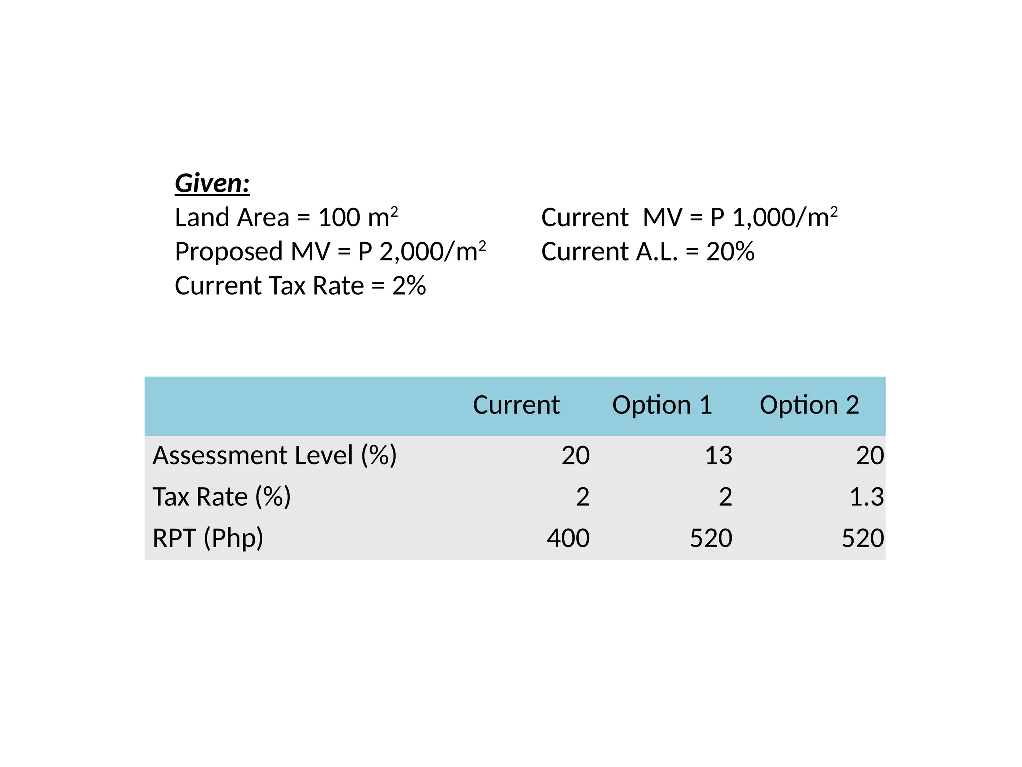
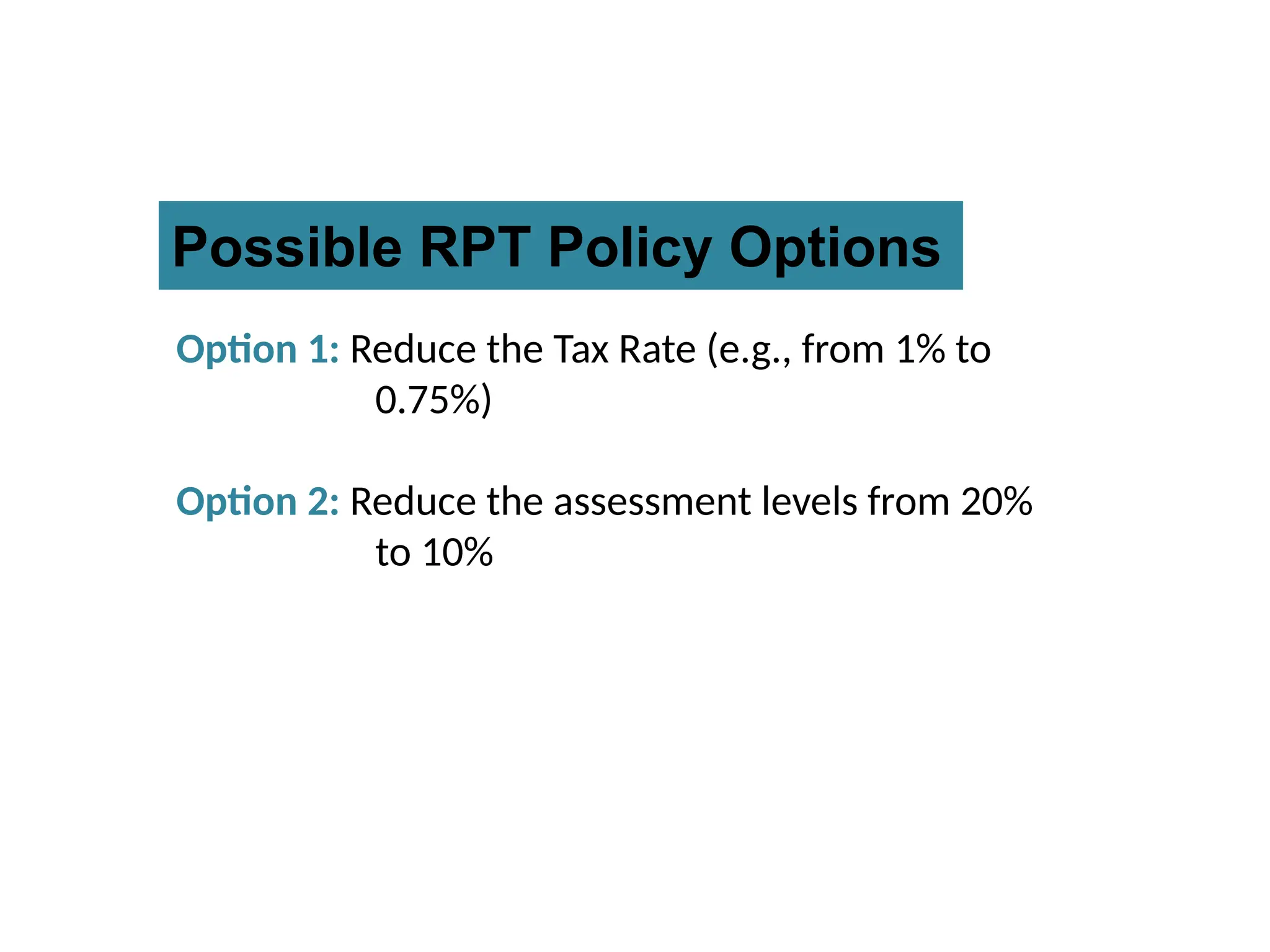
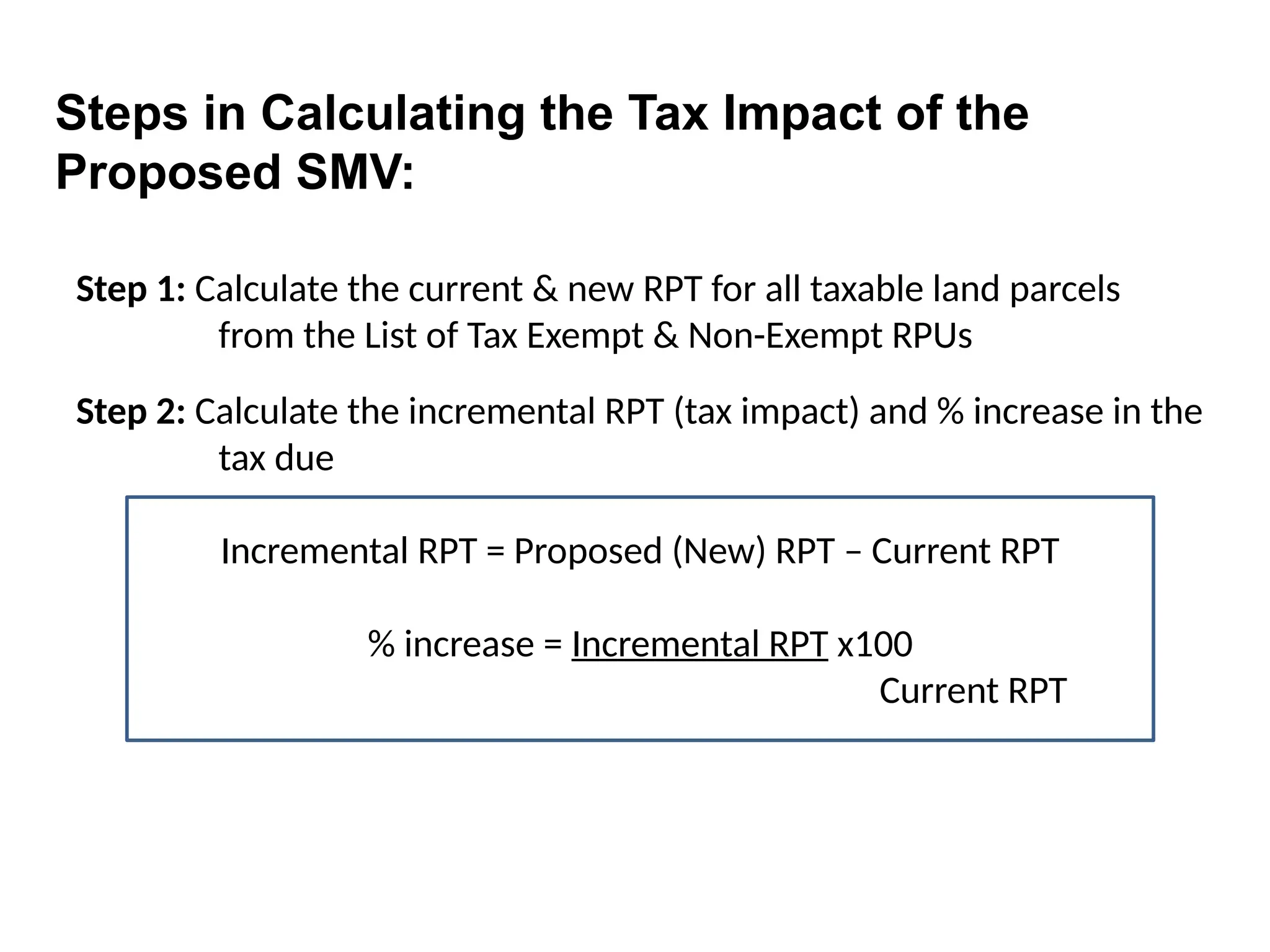
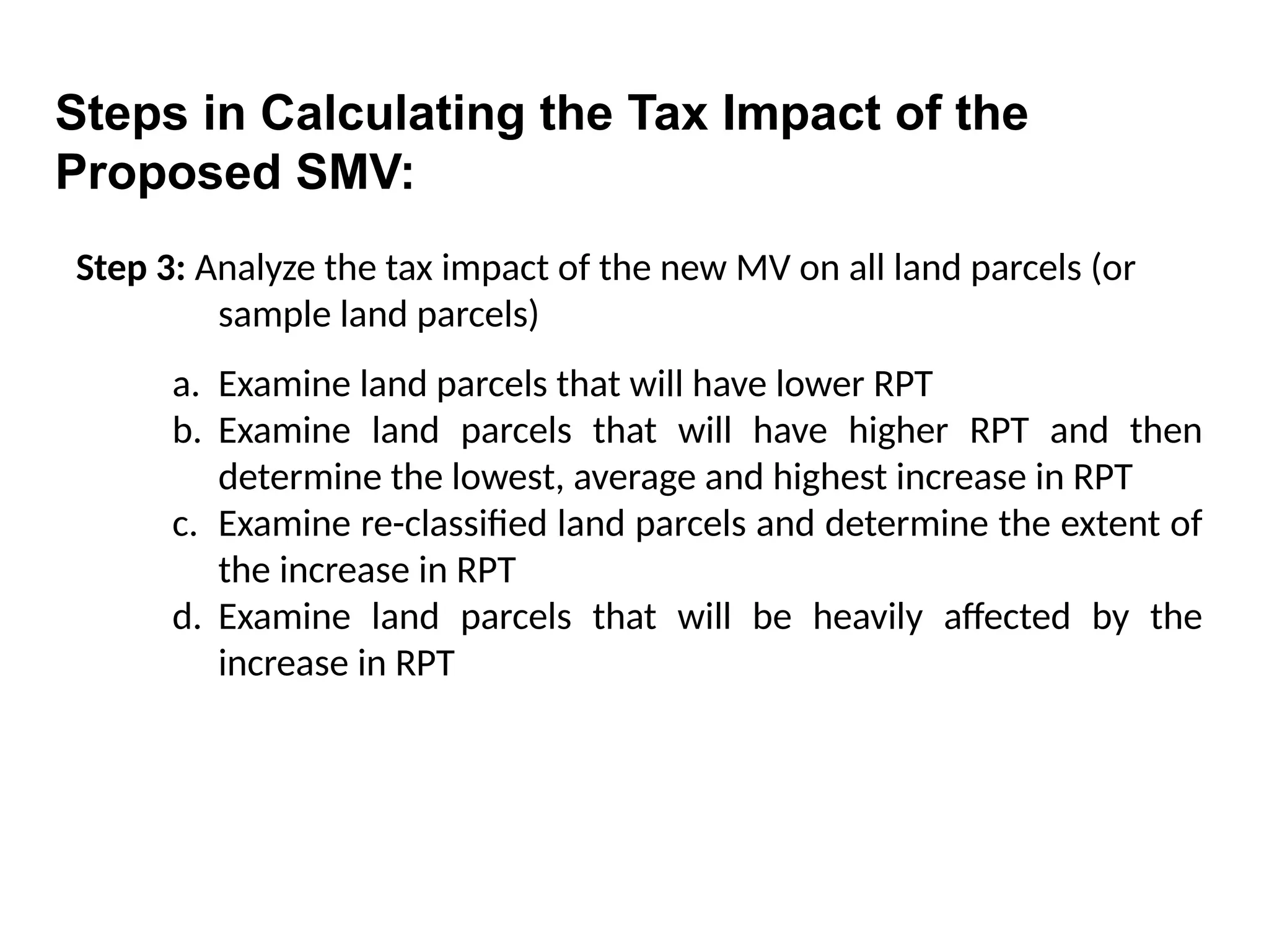
4.7 Tax Impact Study
72.
• SMVs arenot individual valuations
• Establish value ranges encompassing similar type/ value of
land and improvements.
• Value Ranges are set for the different types of real
property units encountered within an LGU. Value ranges
are usually rounded off to their nearest hundreds or
thousands depending upon their interval.
4. Testing of SMV Stage
4.1. Set Interval or Value Ranges
73.
• Several setsof value ranges for land can be found in any
LGU, which includes:
• Standard residential lots along the road
• Standard lots within first class subdivisions
• Standard lots in second class subdivisions
• Standard lots in a general residential area
• Standard second grade retail (commercial) lots
• For buildings, the ranges could include:
• Commercial/Industrial for each type of
construction
• Residential for each type of construction
4. Testing of SMV Stage
4.1. Set Interval or Value Ranges
74.
• Plot thegeographic distribution of the unit values in a
map.
• Allocate the range of values to all the street frontage,
sub-market, and properties within a particular market
area
4.2. Craft the Working Land Value Map
4. Testing of SMV Stage
75.
• Test thevalue of a particular property in the sub-market
area by using the SMV.
• The actual sale of the property may not necessarily align
with the SMV because of the adjustments on the
ranges.
• Check the SMV of adjoining LGUs against the proposed
SMV for consistency of values.
4. Testing of SMV Stage
4.3. Test the Developed SMV
4.4. Check the Values of Adjoining LGUs
76.
• Whenever adjustmentsare made, the adjusted
SMV should be re-tested.
4.6 Prepare Final Draft of SMV
• After testing and re-testing the SMV, prepare the
final draft following the required forms and
formats as prescribed by the DOF-BLGF.
• The SMV can be proposed and recorded on the
land value maps of each barangay.
4. Testing of SMV Stage
4.5. Adjust the Developed/Proposed SMV
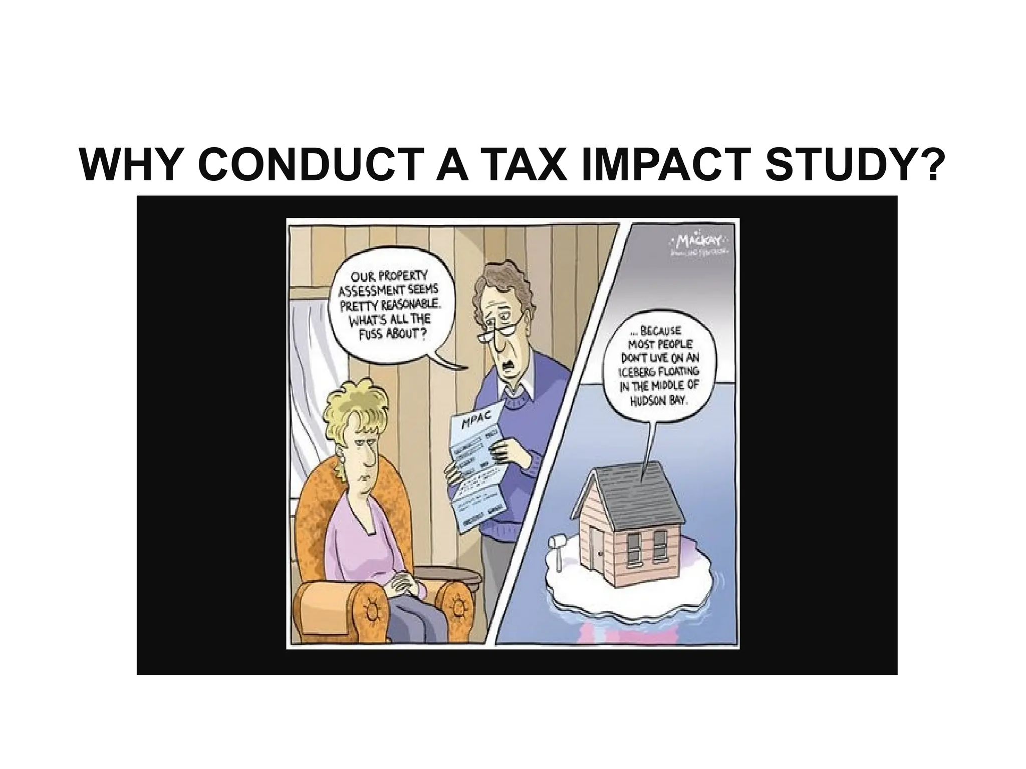
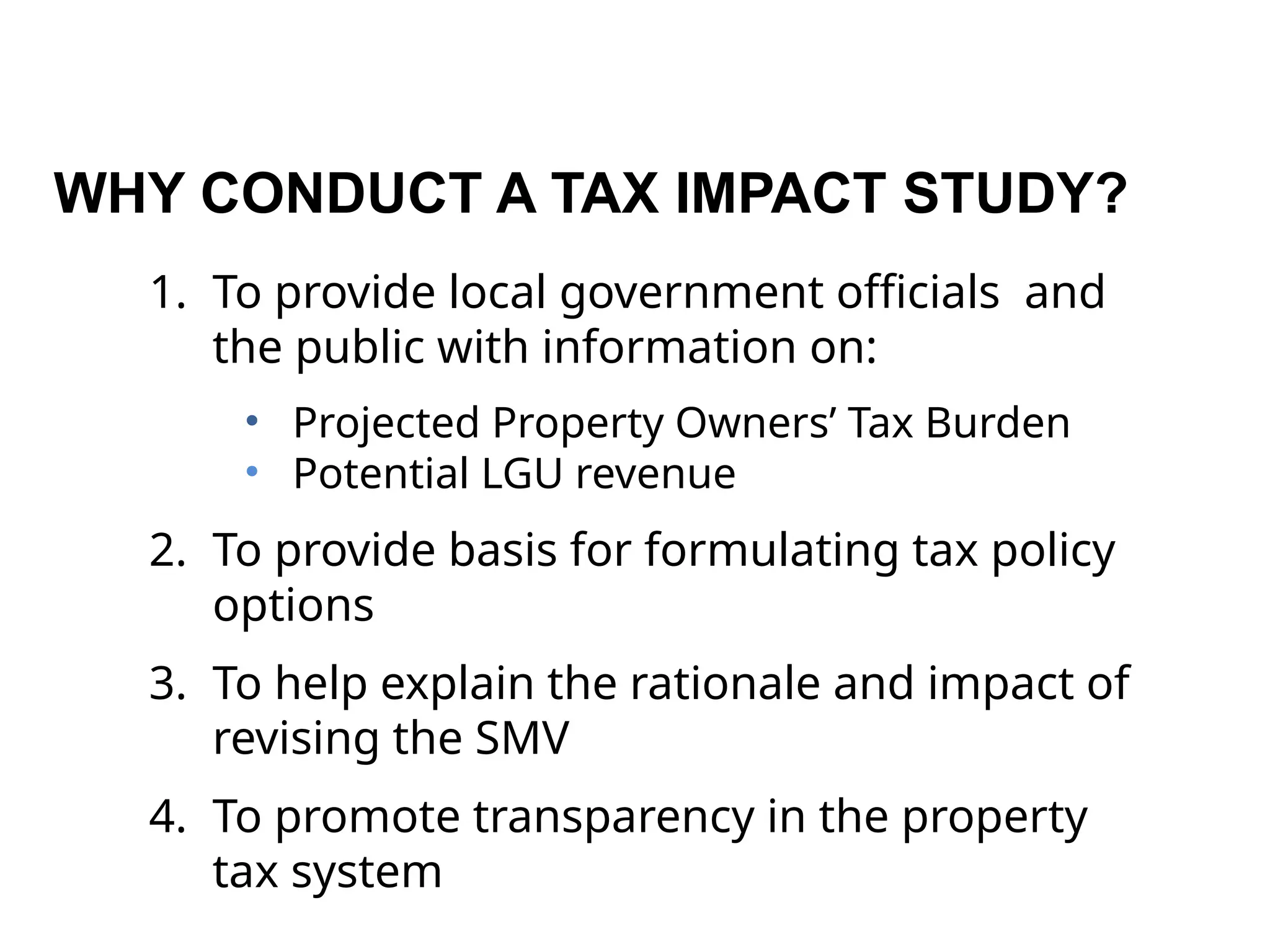
77.
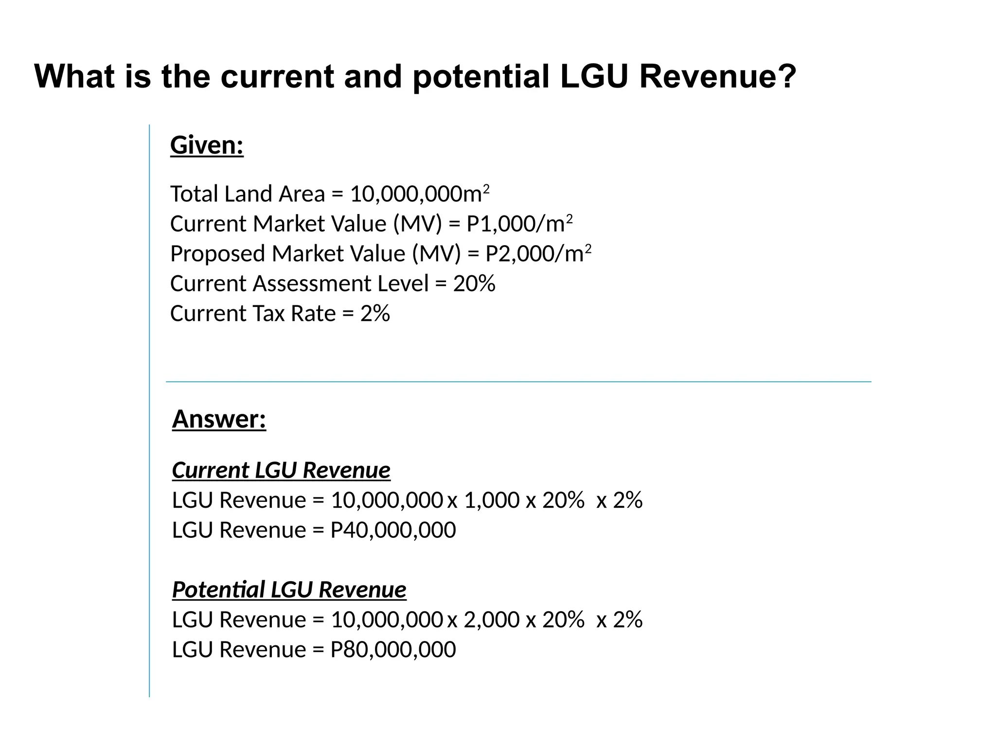
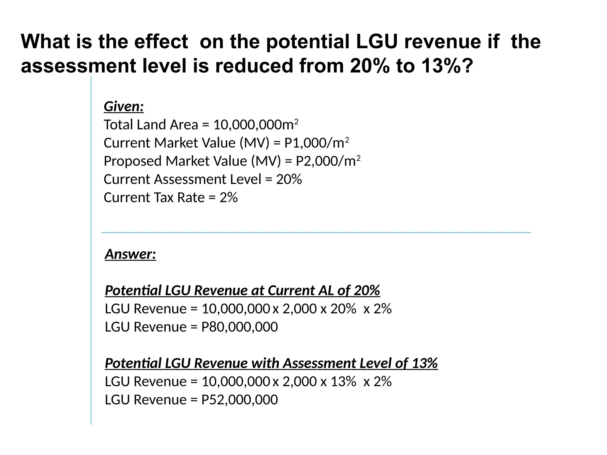
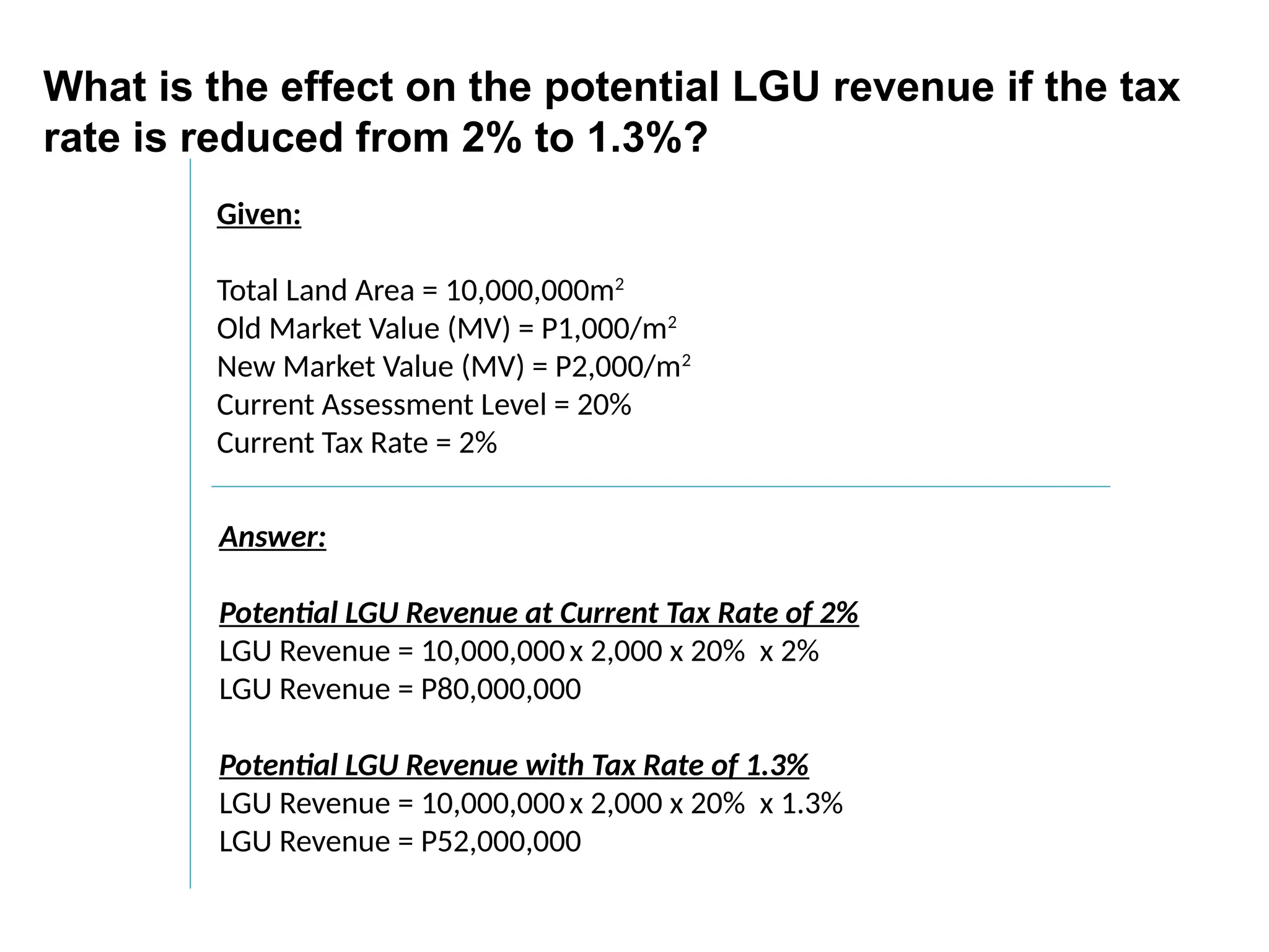
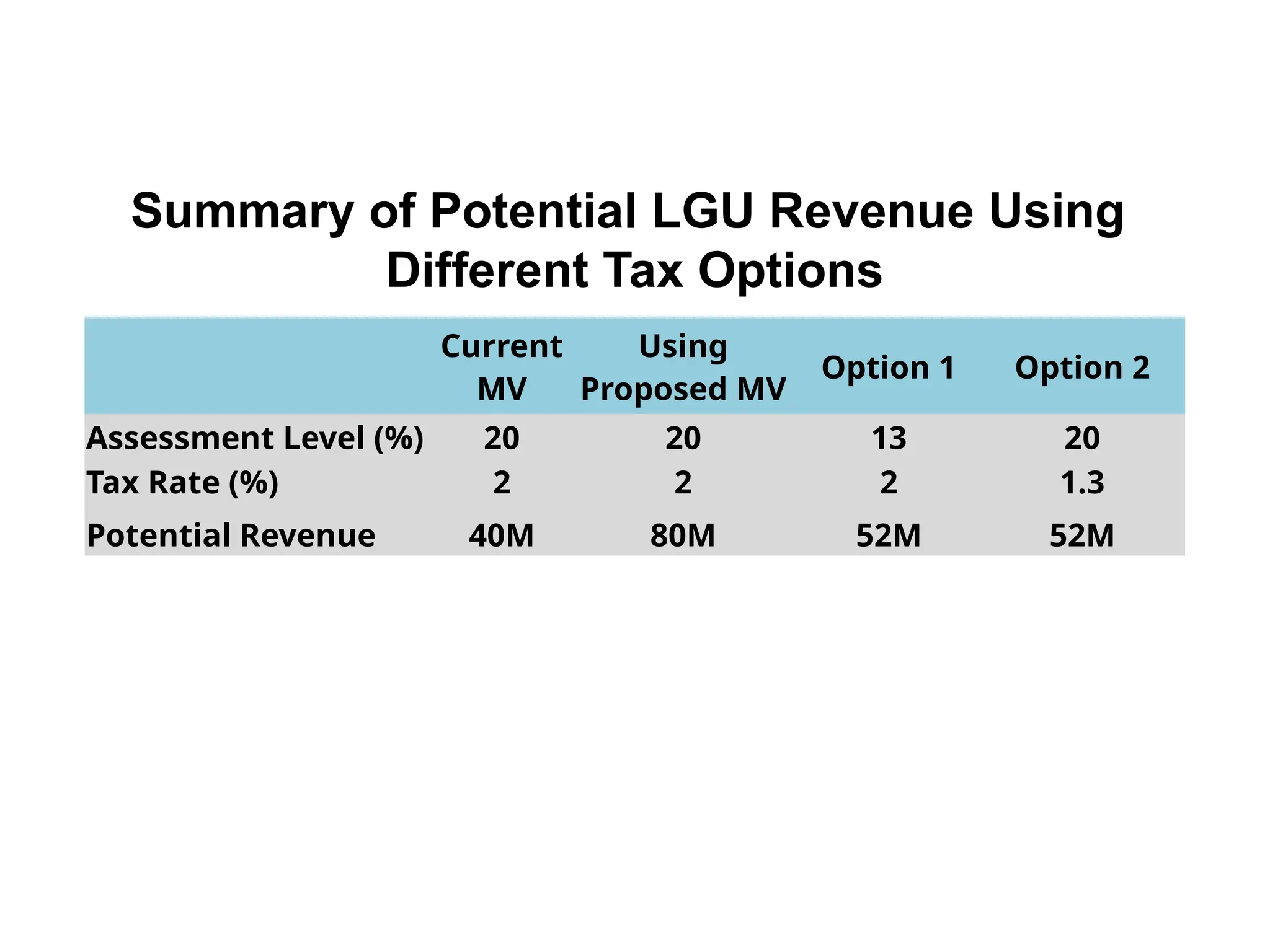
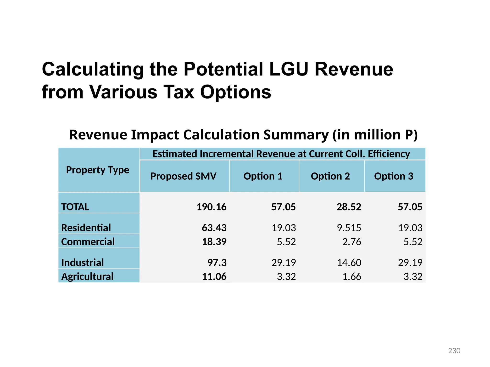
• After completingthe SMV, prepare a tax impact study to
provide an early guide on the effect of the revision.
• A tax impact study will provide the LGU with good
information on the potential revenue and outcomes of
the revision, as well as, being a source of information for
LGU’s Tax Policy.
4. Testing of SMV Stage
4.7. Prepare Tax Impact Study
Residential Land –land principally devoted to
habitation
Commercial Land – land devoted principally for profit
and is not classified as agricultural, industrial,
mineral, timber, or residential land
Industrial Land – land devoted principally to industrial
activity as capital investment and not classified as
agricultural, commercial, timber, mineral or
residential land
Classification of Urban
Lands
(Section 199, RA 7160)
80.
The Concept ofHighest And
Best Use (HABU):
The PVS defines highest and best use as “the
most probable use of a property” which is:
• Physically possible,
• Appropriately justified,
• Legally permissible,
• financially feasible, and
• results in the highest value of the
property being valued
Sales Comparison Approach
EconomicPrinciples Used in the Sales Comparison
Approach
• Competition
• Substitution
• Supply
• Demand
• Highest and Best Use
84.
Market Assumptions
• Sellerswill not take less than present
market value (PMV) of similar property
• Buyers will not pay more than PMV of
similar property.
85.
GIVEN:
Sub-Market Area 1= Residential
No. of Land RPUs = 850
Sample size = 5% = 42 sales
Valid data = 32 sales
Manner of selection = Systematic sampling
(i.e., every 20th
RPU was selected)
DETERMINE MARKET VALUE AND ADJUSTMENT
FACTORS.
Development of SMV Using Sales
Comparison Approach: Prepare an SMV for a
predominantly residential area
Determine the averageinterval.
Average interval = Intervals / number of intervals
∑
Average interval = 113% ÷ 31 = 3.65% say 5%
Determine the ranges using an interval of ±5% or ±0.05.
A B C D
Range
Low 5%
(Php)
Mid
(Php)
High 5%
(Php)
1 1,425 1,500 1,574
2 1,575 1,700 1,784
… … … …
12 4,305 4,500 4,724
13 4,725 5,000 5,249
Range #1:
Assume midpoint = 1500 (C1)
B1 = C1x(1-0.05) = Php1,425
D1 = C1x(1+0.05)-1 = Php1,574
Range #2:
B2 = D1+1 = 1,574+1 = Php1,575
C2 = B2x(1+0.05) = Php1,700 (rounded)
D2 = C2x(1-0.05)-1 = Php1,784
Continue computing until last row.
Count the number of sales with UVs that fall within the range (Freq).
90.
A B CD E
Range Low 5% Mid High 5% Frequency
1 1,425 1,500 1,574 1
2 1,575 1,700 1,784 0
3 1,785 1,900 1,994 1
4 1,995 2,100 2,204 1
5 2,205 2,300 2,414 1
6 2,415 2,500 2,624 2
7 2,625 2,800 2,939 6
8 2,940 3,100 3,254 8
9 3,255 3,400 3,569 6
10 3,570 3,700 3,884 3
11 3,885 4,100 4,304 2
12 4,305 4,500 4,724 0
13 4,725 5,000 5,249 1
Count the number of sales with UVs that fall within the range
and record under column E.
91.
Limit the numberof ranges by combining UVs with lower frequencies.
Plot the frequencies (column E) and the midpoints (column C) in a graph.
92.
Range Mid (Php)Freq
1 1,500 1
2 1,700 0
3 1,900 1
4 2,100 1
5 2,300 1
6 2,500 2
7 2,800 6
8 3,100 8
9 3,400 6
10 3,700 3
11 4,100 2
12 4,500 0
13 5,000 1
Combine ranges with very low frequencies.
Range Low Mid High
1 1,425 1,600 1,784
2 1,785 2,100 2,414
3 2,415 2,500 2,624
4 2,625 2,800 2,939
5 2,940 3,100 3,254
6 3,255 3,400 3,569
7 3,570 3,700 3,884
8 3,885 4,500 5,249
To combine ranges, compute the average
of the mid values then round-off.
When there are too many ranges, ranges may be combined. (e.g., ranges 1
& 2, 3 to 5 and 11 to 13)
Warning: Collapse ranges carefully. The
interval between a midpoint
increases, thus, can overvalue or
undervalue properties
inappropriately.
93.
Sort the midpointsfrom highest to lowest and assign sub-class labels.
Sub-class Unit Value
R1 4,500
R2 3,700
R3 3,400
R4 3,100
R5 2,800
R6 2,500
R7 2,101
R8 1,600
94.
% Adjustment lowland
= (UV sale 22-UV sale 9)/UV Sale 9 x 100%
= (2,500-3,000)/3,000 x 100% = -17%
% Corner Lot
= (UV sale 28-UV sale 9)/UV Sale 9
= (3,333-3,000)/3,000 x 100% = +11%
Base lots: Sales 9, 11 and 23
Rounded unit value of base lot = P3,000
(UV9 + UV11 + UV23) ÷ 3 = P3,051
Compute for Adjustment Factors:
95.
Sale Sale PriceLand Area Unit Value Description
9 600,000 200 3,000 Flat land, inside lot, no view or other factor
11 550,000 180 3,055 Flat land, inside lot, no view or other factor
22 500,000 200 2,500 Inside lot, land drops from road to 1.5 meters
23 620,000 200 3,100
Almost flat land, slightly slopes down from
road
28 600,000 180 3,333 Flat lot, no view, located on good corner.
21 725,000 200 3,625
On higher part of subdivision, slight slope
from road, has very good view
12 495,000 180 2,750
Flat corner lot but near to old railway line and
squatters
30 700,000 200 3,500 Good flat piece of land on main road
Analyze the given data and identify base lots.
Determine adjustment factors and criteria using selected items
from sales data.
96.
% Adjustment elevatedland
= (3,625-3,000)/3,000 x 100% = +20%
% Blighted lot (squatters) with corner influence
= (3,000x111%) = 3,333 (with Corner
Influence)
= (2,750-3,333)/3,333 x 100% = -17.5%
% Effect to Main Road
= (UV sale 30-UV sale 9)/UV Sale 9 x 100%
= (3,500-3000)/3,000 x 100% = +16%
Compute for Adjustment Factors: (cont.)
97.
• Base unitvalue = Php3,000/m2
(Sales 9, 11, 23)
• Sloping down = deduct 16% (Sale 22)
• Corner lots = add 11% (Sale 28)
• With a view = add 20% (Sale 21)
• Blighted Status (Squatters) = deduct 17% (Sale
12)
• Lots along main road = 16% higher (Sale 30)
Results of Analysis:
98.
Sale Sale Price
Land
Area
UnitValue Description Comment
9 600,000 200 3,000
Flat land, inside lot, no view or other
factor
May establish unit value
11 550,000 180 3,055
Flat land, inside lot, no view or other
factor
May establish unit value
(Sale 9)
22 500,000 200 2,500
Inside lot, land drops from road to 1.5
meters
17% drop in price
23 620,000 200 3,100
Almost flat land, slightly slopes down
from road
May establish unit value
(Sale 9)
28 600,000 180 3,333
Flat lot, no view, located on good
corner.
Corner lot achieved 11%
additional value
21 725,000 200 3,625
On higher part of subdivision, slight
slope from road, has very good view
Higher lot with view adds
20% to value
12 495,000 180 2,750
Flat corner lot but near to old railway
line and squatters
Shows reduction in price
17.5% from standard corner
price.
30 700,000 200 3,500 Good flat piece of land on main road
Main road location indicates
16% increase over base
price.
SUMMARY
99.
Criteria for Sub-Classificationof Residential Lands (from the
sample data):
R1 R2 R3
Along main road
Along interior
road with view
Relatively flat
Along interior roads
No View
Relatively flat
…
100.
Adjustment Factors forResidential Lands:
• Corner Influence = +11%
• Sunken Lots less than 1.5m = 0% (No
adjustment)
• Sunken lots at 1.5 m or more = -16%
• Blighted Status (presence of squatters) = -17%
101.
Example of amore comprehensive criteria for a sub-
class:
I. FIRST CLASS RESIDENTIAL LANDS
1. Located along concrete road
2. Area where top grade apartment or residential buildings
are predominantly situated
3. Public utility, transportation facilities are exceptionally
regular toward major trading centers
4. Located next to commercially classified lands
5. Water, electric and telephone facilities are available
6. Commands the highest residential land value in the city
7. Free from squatters
• Analyzing standardlots in a general area may
result in a Time Adjustment Table.
• Every adjustment builds up potential errors,
therefore, the best sales to use are arm’s length
sale of an almost identical property.
• Time adjustment studies should be conducted as
close to the valuation date as possible.
Characteristics:
Referred to as Indexing
Analysis of the change in value over the period from
which sales are collected
Property sales used as evidence for general revision
may be adjusted to prices at valuation date
Adjustments for Time
NOTE the July2005 increase, no movement in October
2005 and the downward trend in April 2006.
Abnormal sales may be discarded.
Land Sales Record – Various Purok Barangay Poblacion
Quarter/Year Analyzed U. Value Total % Increase Q % Increase
Jul-05 2,650 117.7 12.3
Oct-05 2,650 117.7 0.0
Jan-06 2,750 121.4 3.6
Apr-06 2,700 119.5 -1.9
Check abnormalities in the pattern
106.
Determine the expectedunit values as of May 2007.
Sub-Market Area Date of Sale Unit Value
1 May 05 2,450
2 July 05 3,000
3 Feb 06 4,000
4 Oct 04 2,750
Application:
Given 1. Sale per sub-market area (some puroks) in the
same Poblacion:
107.
• Current date
incrementfrom base
date = 29.9%
• Benchmark = May
2007 select closest =
April 2007
Available Sales
Sub-Market
Area
Date of
Sale
Unit
Value
1 May 05 2,450
2 July 05 3,000
3 Feb 06 4,000
4 Oct 04 2,750
Land Sales Record – Purok 1, Barangay Poblacion
Quarter/
Year
Analyzed U.
Value
Q %
Increase
Total %
Increase
Apr-04 2,200 100.0
Jul-04 2,250 2.2 102.2
Oct-04 2,275 1.1 103.3
Jan-05 2,300 1.1 104.4
Apr-05 2,325 1.1 105.5
Jul-05 2,650 12.3 117.7
Oct-05 2,650 0.0 117.7
Jan-06 2,750 3.6 121.4
Apr-06 2,700 -1.9 119.5
Jul-06 2,800 3.6 123.1
Oct-06 2,900 3.4 126.6
Jan-07 2,925 0.9 127.4
Apr-07 3,000 2.5 129.9
Sample Time Adjustment Table
108.
Available
Date of Sale
%Increment from Available Date of Sale to May 2007
Sub-Market
Area 1
Sub-Market
Area 2
Sub-Market
Area 3
Sub-Market
Area 4
May 05
129.9-105.5 =
24.4%
n/a n/a n/a
July 05 n/a
129.9-117.7 =
12.2%
n/a n/a
Feb 06 n/a n/a
129.9-121.4 =
8.5%
n/a
Oct 04 n/a n/a n/a
129.9-103.3
= 26.6%
% Increment from Available Date of Sale:
= Total Increment Benchmark Date – Total Increment Date of Sale
Sample % Increment from Base Value vis-a-vis Available Date of Sale within
Similarly Situated Sub-Market Areas
109.
Available
Date of Sale
ExpectedUnit Value as of May, 2007 (Current Date)
Sub-Market
Area 1
Sub-Market
Area 2
Sub-Market
Area 3
Sub-Market
Area 4
May 05
2,450x1.244 =
3,047 or 3,000
n/a n/a n/a
July 05 n/a
3,000x1.122 =
3,366 or 3,300
n/a n/a
Feb 06 n/a n/a
4,000x1.085 =
4,340 or 4,300
n/a
Oct 04 n/a n/a n/a
2,750x1.1266=
3,481 or 3,400
Expected Unit Value at Current Date
Expected Unit Value = Unit Value x (1 + % increment from base value)
110.
Sub-Market
Area
Date of Sale
UnitValue at
Date of Sale
Expected Unit Value
in May 2007
1 May 05 2,450 3,000
2 July 05 3,000 3,300
3 Feb 06 4,000 4,300
4 Oct 04 2,750 3,400
As of May 2007, the lots were valued as:
A method usedto determine the value of one component of a
property by deducting the value of other components from
the full value or sale price.
Land Residual Technique
113.
Given:
Parcel 1
Land Area= 200m2
Total Building Area (2S)= 180m2
Building Age = New
Selling Price = Php 1.85 million
With Block fences = 60lm
Paving = 83m2
Parcel 2
Land Area = 180m2
(9m x 20m)
Unit Value = Php 3,000/m2
Building Age = 5 years old
Annual Depreciation Rate = 5.5%
Total Building Area (2S)= 140 m2
Selling Price = Php 1.45 million
With Block fences = Php1,200/lm
Conditions:
Lands are similarly situated. Buildings are similarly constructed.
Paving = Php800/m2
Determine the land unit value of Parcel 1.
Application:
114.
Determine land valueand building value of Parcel 2.
Land Value = 180m2
x Php 3,000/m2
= Php 540,000
Block Fences = Perimeter x Php1,200/lm
= 58 lm x Php1,200/lm
= Php 69,600
Depreciated Building Value = 1,450,000 – 540,000 – 69,600
= Php 840,400
Building Value New = Php 840,400 ÷ (1.0-0.055)
= Php 888,312
Building Unit Value = Php 888,312 ÷ 140m2
= Php 6,352/m2
= Php 6,500/m2
115.
Apply the unitvalue of building to parcel 1:
Value of Building = 180m2
x Php 6,500/m2
= Php 1,170,000
Value of Fence = 60 lm x Php1,200/lm = 72,000
Value of Pavement = 83 m2
x Php800/m2
= Php 66,400
Value of Land (Parcel 1) = 1,850,000 – 1,170,000 – 72,000
– 66,400
= Php 541,600
Unit Value of Land = Php 541,600 ÷ 200m2
= Php 2,708/m2
= say Php 3,000/ m2
116.
NOTES:
By using thesame residual technique in extracting the
value of other lands, a schedule of market value can be
developed.
The criteria are determined by the conditions of the land.
Adjustment factors are determined by the physical
characteristics of the land.
Triangular and IrregularLots
Appraise using highest and best use or most probable use.
Reduction in value due to shape will also be influenced by
size of the parcel.
i.e., small, awkwardly shaped parcels may suffer large drops in
value due to having very little use while large, irregular parcels
may be valued as other regular lots.
It has yet to be proven that size affects value based on local
conditions.
119.
Common Approach toValue:
Base on the street - 2/3 x Market
Value of rectangular lot
Apex on the street - 1/3 x Market
Value of rectangular lot
Trapezoidal/Irregular Lots =
Rectangle + Triangle
Accurate approach: Use Technical
Description
Triangular and Irregular Lots
120.
Stripping Method
Land atvarious distances from the front of the site is
allocated with a different value as a percentage of the value
of land at the front.
Usually used for large lots.
121.
There are mixedviews whether this method reflects market
dynamics.
It can be considered as a valid method in adjusting valuation IF
pattern exists and proven that it applies to many transactions.
“The stripping method shall not be applied on commercial
and industrial properties”
(Assessor’s Manual, p. 111)
Appropriate adjustment for commercial and industrial properties
may be done using other criteria or adjustment factors.
Stripping Method
122.
Establishing a standarddepth:
• Analyze a set of homogeneous properties
grouped by frontage and depth.
• Compare sales values.
• If property values fall as the depth gets longer,
then value is affected by depth.
• Standard depth varies between market areas.
Stripping Method
123.
To illustrate:
Basic Assumptions:
(1)Standard depth = 35m
(2) Base price for a 35m deep lot is Php15,000.00/m2
(Established by Sale 2 and 3)
(3) All Lots were sold recently
(4) Frontage = 15 meters (except for lots 7 & 8)
Analyze each sale and determine if there is a pattern
evolving from these transactions.
Stripping Method
124.
Sale
Front x
Depth
Area
(m2
)
Lot Price
Unit
Value/
m2
ComputationsAnalysis
1 15 x 25 375 6,000,000 16,000 16,000/15,000 = 1.07
Lot is smaller than typical and
reflects slightly higher than
typical unit value
2 15 x 35 525 7,875,000 15,000 15,000/15,000 = 1
The typical depth for this
locality is 35m. There is no
need for stripping in this lot.
3 15 x 35 525 7,875,000 15,000 15,000/15,000 = 1
The typical depth for this
locality is 35m. There is no
need for stripping in this lot.
4 15 x 42 630 9,135,000 12,000
Base lot size, 525m2
x P15,000 = P7.875M
Sale of P9.135M –
P7.875M = P1.26M
Therefore, rear strip
= P1.26M/(7mx15m)
= P12,000/m2
12,000/15,000 = 0.8
Shows 20% lesser in value
than front strip
Stripping Method
Analysis for Stripping Method
125.
Sale
Front x
Depth
Area
(sqm)
Lot Price
Unit
Value/
m2
ComputationsAnalysis
5 15 x 50 750 10,350,000 11,000
Base lot of 525m2
x P15,000
= P7.875M
Sale of P10.35M – P7.875M
= P2.475M
Rear strip has a value of
P2.475M/(15m x 15m) =
P11,000/m2
UV for rear strip =
P11,000/m2
11,000/15,000 = 0.733
There was a drop in value by
26.7%
6*
(15x30)+
(30.1x2)
480 8,280,000 17,250
480m2
x P15,000 = P7.2M
P8.28M/P7.2M = 1.15
Corner lot shows additional 15%
value from basic lot
7**
30.1x
(17(N), 20
(S), 30(W))
292.5 4,095,000 14,000 14,000/15,000 = 0.93
This lot will not be considered
for stripping since it has a
different frontage and side
street
* Irregular corner Lot ** Slightly irregular corner lot
Stripping Method
Analysis for Stripping Method (cont.)
126.
*** Slightly irregularcorner lot
Sale
Front x
Depth
Area
(m2
)
Lot Price
Unit
Value/
m2
Computations Analysis
8***
N(19x30),
W (30.1m),
S (17m)
540 9,072,000 16,800
540m2
x P15,000 = P8.1M
P9.072M – P8.1M =
P972,000
Additional value of a
corner lot: P972,000
(P972,000/540m2
= 1,800
additional unit value)
18,000/15,000 = 1.12
An additional 12% value from a
basic lot
Stripping Method
Analysis for Stripping Method (cont.)
127.
From the previoustable, the following conclusions
can be made:
• Unit value in the area is Php15,000/m2
• Lots exceeding the 35m standard depth
showed a lower unit value, thus, was affected
by depth.
• Corner lots are not affected by stripping.
Stripping Method
128.
Physical Factors asBasis for the
Development of Adjustment Factors
• Adjustments needed to allow for physical differences
when valuing properties
i.e., size, view, location, shape, elevation, topography,
access
• A common method is the use of matched pairs
Requires that sales are similar in all, except 1,
characteristics
Validate adjustment by comparing a succession of other
matched pairs
Create Table of Adjustments after several adjustments
were made
129.
Property Conditions asBasis for the
Criteria in the Classification and Sub-
Classification of Lands
• Basis for classification are the limitations of
land use and value of sales in a particular
area, given all conditions are equal
• Physical effects of properties (i.e.,
applicable to a number of properties) may
also be used as criteria
130.
Establishing Land ValueMaps
• Visible and effective tool for displaying values
deduced from actual land and improved sales.
• Can be any form of LGU base map but should include
details on location and, if possible, show actual
streets/roads.
• Tool for appraisers with index on benchmarks and
market data.
131.
Preparation of LandValue Maps
Working Land Value Maps
• Shows range of values within a sub-market area detailed
along streets and particular locations
• Information on maps include the benchmarks, all sales,
recent asking prices, offers, zoning, road information,
statistical building class, depreciation and other
appraisal data.
• Factors affecting value are usually color-coded
Final Land ValueMaps
• Final values are plotted along the streets or peculiar
locations on the map
• Land value maps work efficiently on urban areas where
there are road and street networks
• Also useful for agricultural lands
Preparation of Land Value Maps
134.
Schedule of MarketValues (Barangay Poblacion)
Land Value Maps
Final Land Value Map:
Valuation is focusedon the utility of the property/site,
i.e., the intended use of the property for a typical buyer
from a typical seller.
Considerations in valuing commercial land:
• Location
• Optimal size
• Flow and Volume of Traffic
• Corner Influence
• Public facilities and amenities
Developing SMV for Commercial and
Industrial Lands
137.
Considerations in valuingindustrial land:
• Zoning
• Large Area
• Availability of private and public utilities
Developing SMV for Commercial and
Industrial Lands
138.
Specific Valuation Approaches
•The correct valuation approach is that which
will be used by buyers and sellers in the
property market
• Nature of improvements makes valuation more
complex
• Valuation with emphasis on permitted use and
geographic factors
Developing SMV for Commercial and
Industrial Lands
139.
Ground rent isrent for vacant land.
Process of valuation is straightforward, not complicated by
operating expenses
Difficulty with capitalizing ground rent is in determining
capitalization rate
To determine a reliable rate, locate a comparable site that
was sold which can be valued by sales comparison, and is
also leased.
Income Capitalization Approach: Capitalization of Ground Rent
140.
Ground rents oftenshow a lower capitalization rate than
developed properties due to the durable nature of the
land.
Caution!
Long-term or short-term rent do not often reflect the value of the
land.
Short-term rent – rent for convenience, for purposes of short-term
storage, from owners who do not require the land in the
immediate future
Income Capitalization Approach: Capitalization of Ground Rent
141.
Lot Dimensions
Land
Area
Net RentDescription
1 10m x 20m 200 42,000
Flat land, inside lot, no view or other
factor
2 8.5m x 20m 170 35,000
Flat land, inside lot, no view or other
factor
3 8m x 20m 160 26,000
Inside lot, land drops from road by
1.5 m (i.e., slopes down)
4 7.5m x 20m 150 31,000
Almost flat land, slight fall from road
(slope down)
5 10m x 20m 200 46,000
Flat lot, no view, located on good
corner
Income Capitalization Approach: Capitalization of Ground Rent -
Application
Given:
List of Ground Rent
142.
Formula:
V = I/ CR
Where:
V = Market Value
I = Net Income/Rent
CR = Capitalization Rate
CR = I / V x 100
Income Capitalization Approach: Capitalization of Ground Rent -
Application
143.
Estimate the CRfrom known valid sales and rentals
Sale Area
Market
Value
Net Annual
Rent Capitalization Rate
A 150 2,000,000 240,000 12.0
B 180 2,000,000 180,000 9.0
C 100 1,100,000 120,000 10.91
D 200 3,800,000 360,000 9.47
Average Capitalization Rate 10.35% or 10%
Income Capitalization Approach: Capitalization of Ground Rent -
Application
144.
Lot
(a)
Land
Area
(b)
Net Mo.
Rent
(c)
CR
%
(d)
Market
Value
(e)
UV
w/
Inf
(f)
Influences
(g)
Adj.
to UV
(Inf)
(h)
UnitValue
without
Influence
(i)
Rnded
Unit
Value
(j)
1 200 42,000 10 5,040,000 25,200
Flat, inside lot, no other
factor
0% 25,200 25,000
2 170 35,000 10 4,200,000 24,705
Flat, inside lot, no other
factor
0% 24,705 25,000
3 160 26,000 10 3,120,000 19,500 Inside lot, drops to 1.5m -20% 15,600 16,000
4 150 31,000 10 3,720,000 24,800 Almost flat, slight slope 0% 24,800 25,000
5 200 46,000 10 5,520,000 27,600 Flat, no view, good corner +12% 30,912 31,000
(e) = [(c)x 12)]/(d) (f) = (e)/(b) i = (f) x [(100%-(h)]/100
Income Capitalization Approach: Capitalization of Ground Rent -
Application
Determine unit values
145.
Schedule of MarketValues for Commercial Lands
Sub Classification Unit Value
C1 25,000
C2 20,000
C3 15,000
C4 12,500
C5 10,000
C6 7,500
C7 5,000
Income Capitalization Approach: Capitalization of Ground Rent
146.
Sample Criteria forSub-Classification of Commercial Lands:
1st
class
commercial
lands
i. Located along concrete road
ii. Areas where the highest trading activities of the city takes place
iii. Areas where vehicular and pedestrian traffic flow are exceptionally busy
iv. Apparently commands the highest commercial land value in the city
2nd
class
commercial
lands
i. Located along concrete road
ii. Areas where the highest trading, social or educational activities are
considerably high
iii. Areas where all concrete commercial or business buildings are situated
iv. Areas where vehicular and pedestrian traffic flow are considerable busy, but
fall short than that of the 1st
class commercial lands
Etc. . . .
Income Capitalization Approach: Capitalization of Ground Rent
147.
Adjustment Factors:
Corner Influence= +12%
Sunken Lots less than 1.5m = 0%
(No adjustment)
Sunken lots at 1.5m or more = -20%
Income Capitalization Approach: Capitalization of Ground Rent
Other adjustment factors can be determined using
the same method.
148.
NOTE:
Where there areno rental data specific only to the
land, identify similar lands with improvements which
rental adheres more to the land rather than its
improvement.
Example:
• Car Wash
• Parking lots
• Display areas
Income Capitalization Approach: Capitalization of Ground Rent
149.
Pty
Unit
Value
Area
m2
Market
Value
Date
Feature &analyzed effect(UV)
Comments
Corner View Traffic Other
1 6,700 200 1,340,000 Feb-08 Typical Lot
2 7,250 200 1,450,000 Mar-09 +550 High side of Road
3 7,350 210 1,543,500 Apr-09 +650 Good view
4 6,500 280 1,820,000 Apr-09 Typical Lot
5 7,900 200 1,580,000 May-09 +1200 Abuts 1st
Class Subdn.
6 6,750 250 1,687,500 Jun-09 Typical Lot
7 5,750 200 1,150,000 Jun-09 -950 Near busy Intersection
8 7,500 200 1,500,000 Jun-09 +800 Adjoins Main Street
9 8,050 200 1,610,000 Aug-09 +750 +600 Good Corner and view
10 6,550 300 1,965,000 Aug-09 Typical Lot
Sales within the 18-month period unaffected by time (lots 1, 4, 6, 10).
Factors Influencing values of Commercial and Industrial Lands
Unaffected by Time
Sample list of property values unaffected by time with features and
analyzed effects
150.
*Adjustments = averageof feature and analyzed effect per item
Factors Influencing values of Commercial and Industrial Lands
Unaffected by Time
Adjustment factors unaffected by time
Pty
Base Land
Value at
Base Date
(Php/m2
)
Base Land
Area of
Typical lot
(m2
)
Base
Date
Adjustments (Php)*
Corner View Traffic Size Features
775 600 -950 0 1,200
% Adjustments (Average/Base Land Value x 100)
1 6,700 200 8-Feb 12 9 -14 0 18
2 7,250 200 9-Mar 11 8 -13 0 17
3 7,350 210 9-Apr 11 8 -13 0 16
4 6,500 280 9-Apr 12 9 -15 0 18
5 7,900 200 9-May 10 8 -12 0 15
6 6,750 250 9-Jun 11 9 -14 0 18
7 5,750 200 9-Jun 13 10 -17 0 21
8 7,500 200 9-Jun 10 8 -13 0 16
9 8,050 200 9-Aug 10 7 -12 0 15
10 6,550 300 9-Aug 12 9 -15 0 18
151.
Base Land Areafor Locality using typical lot 200
Base land Value at Base Date 6,700
Base Date Feb 08
Adjustments*
%
Adjustment*
*
Corner 775 12%
Views 600 9%
Traffic -950 -14%
Size 0 0%
Features 1,200 18%
* Derived average on feature and analyzed effect per column
** %Adjustment = Average/(Base Land Value) x 100%
(Example: 775/6700 x 100 = 11.6% or 12%)
Effect to a property unaffected by time: Average adjustments
Factors Influencing values of Commercial and Industrial Lands
Unaffected by Time
152.
* Derived averageon feature and analyzed effect per column
** %Adjustment = Average Adjustment/Base Land Value x 100%
Base Land Area for
Locality using typical lot
(1)
200
(4)
280
(6)
250
(10)
300
Ave
Base land Value at Base
Date
6,700 6,500 6,750 6,550
Base Date Feb 08 Apr 09 Jun 09 Aug 09
Adjustments* % Adjustment**
Corner 775 12% 12% 11% 12% 12%
Views 600 9% 9% 9% 9% 9%
Traffic -950 -14% -15% -14% -15% -15%
Size 0 0% 0% 0% 0% 0%
Features 1,200 18% 18% 18% 18% 18%
Resulting Average to unaffected properties 1,4, 6 &10:
Factors Influencing values of Commercial and Industrial Lands
Unaffected by Time
153.
Drafting the SMVfor Residential, Commercial and Industrial Lands:
Sample SMV
Street/ Subdivision Vicinity
2003 2009
Base Value
(Php)
Sub-Class
Base Value
(Php)
Sub-Class
Barangay 1
Street A Road 1 - Road 2
3,500.00 R-4 5,000.00 R-3
2,800.00 I-3 7,200.00 I-2
Street B Street XX - Street YY 5,000.00 R-1 6,000.00 R-2
Interior Lots 2,500.00 R-8
Avenue A Street XY - Street YZ 12,800.00 C-1 20,000.00 C-1
Gen Luna - Street XY 10,300.00 C-3 12,000.00 C-4
Street XY - 1st 300m 8,500.00 C-5 15,000.00 C-3
Street YZ to Port Area 4,000.00 I-1 8,000.00 I-1
Others 4,800.00 R-2 6,000.00 R-2
Subdivision A 6,000.00 R-2
Subdivision B 5,500.00 R-2 7,000.00 R-1
All Blighted Areas
Note: R = Residential, C = Commercial, I = Industrial
At the endof Module 5, the participants will be able to:
1. Identify plant, machinery and equipment that are
included in valuation
2. Learn the valuation methods applicable to plant,
machinery and equipment
3. Apply the appropriate techniques of valuation of
plant, machinery and equipment
OBJECTIVES:
156.
Machinery
“Machinery embraces machines,equipment, mechanical
contrivances, instruments, appliances or apparatus, which may
not be attached, permanently or temporarily to the real
property. It includes the physical facilities for production, the
installations and appurtenant service facilities, those which are
mobile, self-powered or self-propelled, and those not
permanently attached to the real property which are actually,
directly, and exclusively used to meet the needs of the particular
industry, business or activity and which by their very nature and
purpose are designed for, or necessary to its manufacturing,
mining, logging, commercial, industrial or agricultural
purposes.”
[Local Government Code, Section 199]
157.
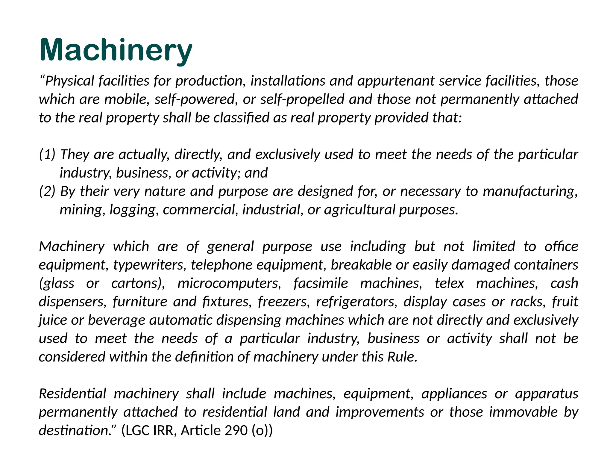
“Physical facilities forproduction, installations and appurtenant service facilities, those
which are mobile, self-powered, or self-propelled and those not permanently attached
to the real property shall be classified as real property provided that:
(1) They are actually, directly, and exclusively used to meet the needs of the particular
industry, business, or activity; and
(2) By their very nature and purpose are designed for, or necessary to manufacturing,
mining, logging, commercial, industrial, or agricultural purposes.
Machinery which are of general purpose use including but not limited to office
equipment, typewriters, telephone equipment, breakable or easily damaged containers
(glass or cartons), microcomputers, facsimile machines, telex machines, cash
dispensers, furniture and fixtures, freezers, refrigerators, display cases or racks, fruit
juice or beverage automatic dispensing machines which are not directly and exclusively
used to meet the needs of a particular industry, business or activity shall not be
considered within the definition of machinery under this Rule.
Residential machinery shall include machines, equipment, appliances or apparatus
permanently attached to residential land and improvements or those immovable by
destination.” (LGC IRR, Article 290 (o))
Machinery
158.
Valuation Approach for
Machineryand Equipment for
RPT Purposes
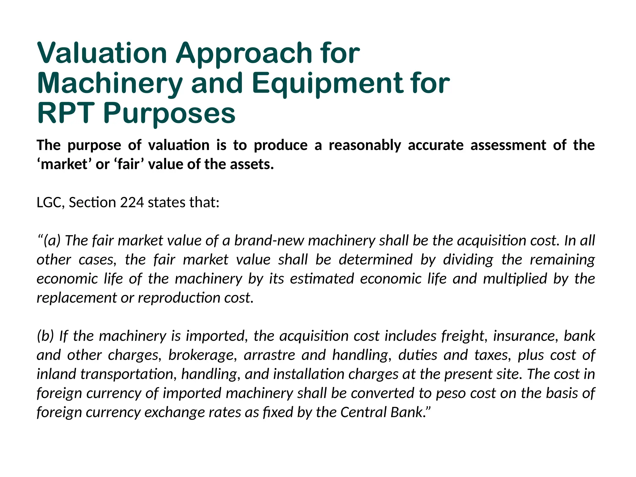
The purpose of valuation is to produce a reasonably accurate assessment of the
‘market’ or ‘fair’ value of the assets.
LGC, Section 224 states that:
“(a) The fair market value of a brand-new machinery shall be the acquisition cost. In all
other cases, the fair market value shall be determined by dividing the remaining
economic life of the machinery by its estimated economic life and multiplied by the
replacement or reproduction cost.
(b) If the machinery is imported, the acquisition cost includes freight, insurance, bank
and other charges, brokerage, arrastre and handling, duties and taxes, plus cost of
inland transportation, handling, and installation charges at the present site. The cost in
foreign currency of imported machinery shall be converted to peso cost on the basis of
foreign currency exchange rates as fixed by the Central Bank.”
159.
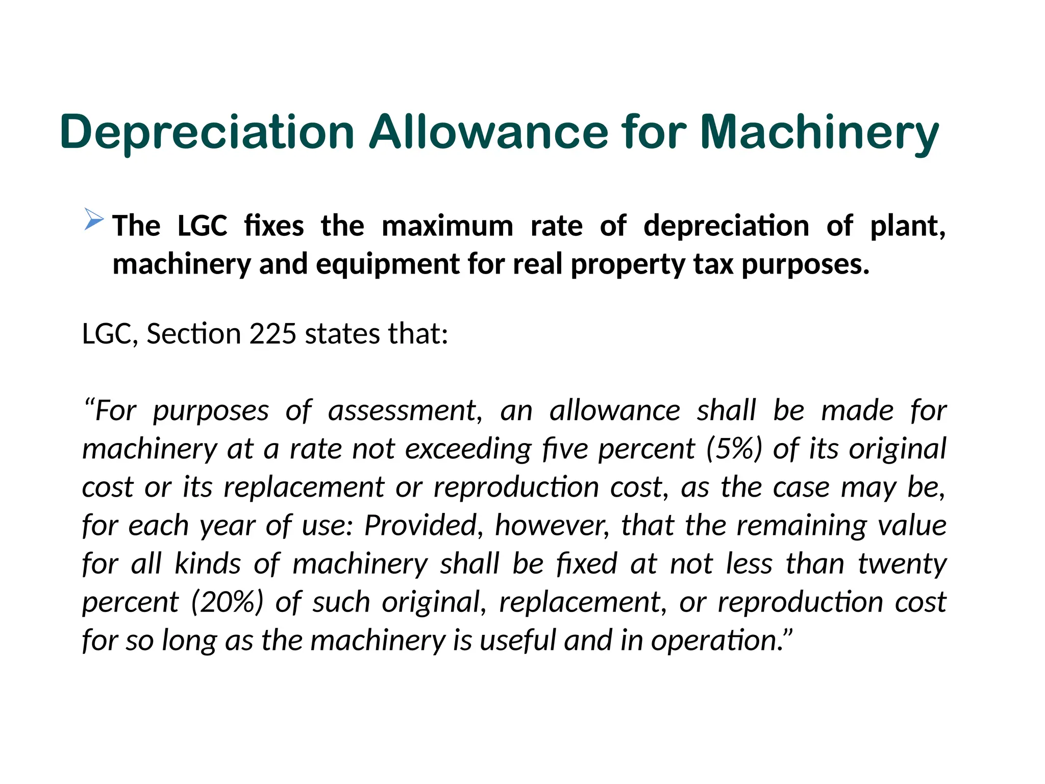
Depreciation Allowance forMachinery
The LGC fixes the maximum rate of depreciation of plant,
machinery and equipment for real property tax purposes.
LGC, Section 225 states that:
“For purposes of assessment, an allowance shall be made for
machinery at a rate not exceeding five percent (5%) of its original
cost or its replacement or reproduction cost, as the case may be,
for each year of use: Provided, however, that the remaining value
for all kinds of machinery shall be fixed at not less than twenty
percent (20%) of such original, replacement, or reproduction cost
for so long as the machinery is useful and in operation.”
160.
Basic Procedure inValuation of Plant,
Machinery and Equipment
1. Conduct thorough inspection of machinery and equipment
2. Determine the basis of valuation/methodology
3. Estimate the replacement cost new if the cost approach is
used
4. Gather and analyze the market data if the market approach is
used
5. Determine the loss in value (depreciation) resulting from
physical deterioration, functional and economic obsolescence
161.
Valuation Methods forMachinery and
Equipment
1. Cost Approach or Depreciated Replacement Cost (DRC)
– cost estimate to replace the asset or group of assets
appraised in accordance with current market prices for
similar assets
2. Sales Comparison or Market Approach – considers
recent prices for similar items, with adjustments on
indicated market prices to reflect the condition and
utility of the appraised items relative to comparable
items in the market
162.
The Cost Approach
Stepsin Using the Cost Approach to Valuation:
1. Estimate the Replacement Cost New (RCN) of the
property as of the date of valuation
2. Deduct the loss in value brought about by depreciation
from all causes to derive the market value of the plant,
machinery and equipment
163.
The LGC requiresthe appraisal of machinery for annual
RPT purposes to be based on its acquisition cost to the
owner, if brand new.
For second-hand or used machinery,
Value = RCN x Remaining economic life
Total economic life
and account for actual condition at reference date.
The Cost Approach
164.
Stage 1: EstimatingReplacement Cost New (RCN)
Two (2) major elements of cost involved in estimating RCN:
1. Direct Costs – costs directly related to the acquisition and
installation of the unit such as basic cost, freight charges,
insurance, bank charges and commission, duties and taxes,
other landing charges and handling and cost of
transportation to site.
2. Indirect Costs – costs not directly related to the acquisition
of a property but relates to the installation and acquisition of
the entire property such as design and engineering, technical
know-how and pre-operating expenses.
The Cost Approach
165.
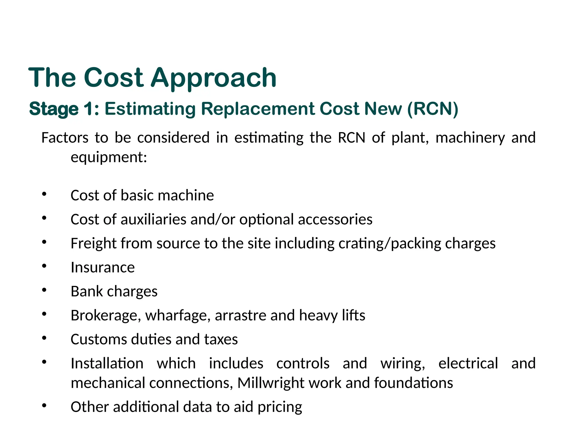
Factors to beconsidered in estimating the RCN of plant, machinery and
equipment:
• Cost of basic machine
• Cost of auxiliaries and/or optional accessories
• Freight from source to the site including crating/packing charges
• Insurance
• Bank charges
• Brokerage, wharfage, arrastre and heavy lifts
• Customs duties and taxes
• Installation which includes controls and wiring, electrical and
mechanical connections, Millwright work and foundations
• Other additional data to aid pricing
The Cost Approach
Stage 1: Estimating Replacement Cost New (RCN)
166.
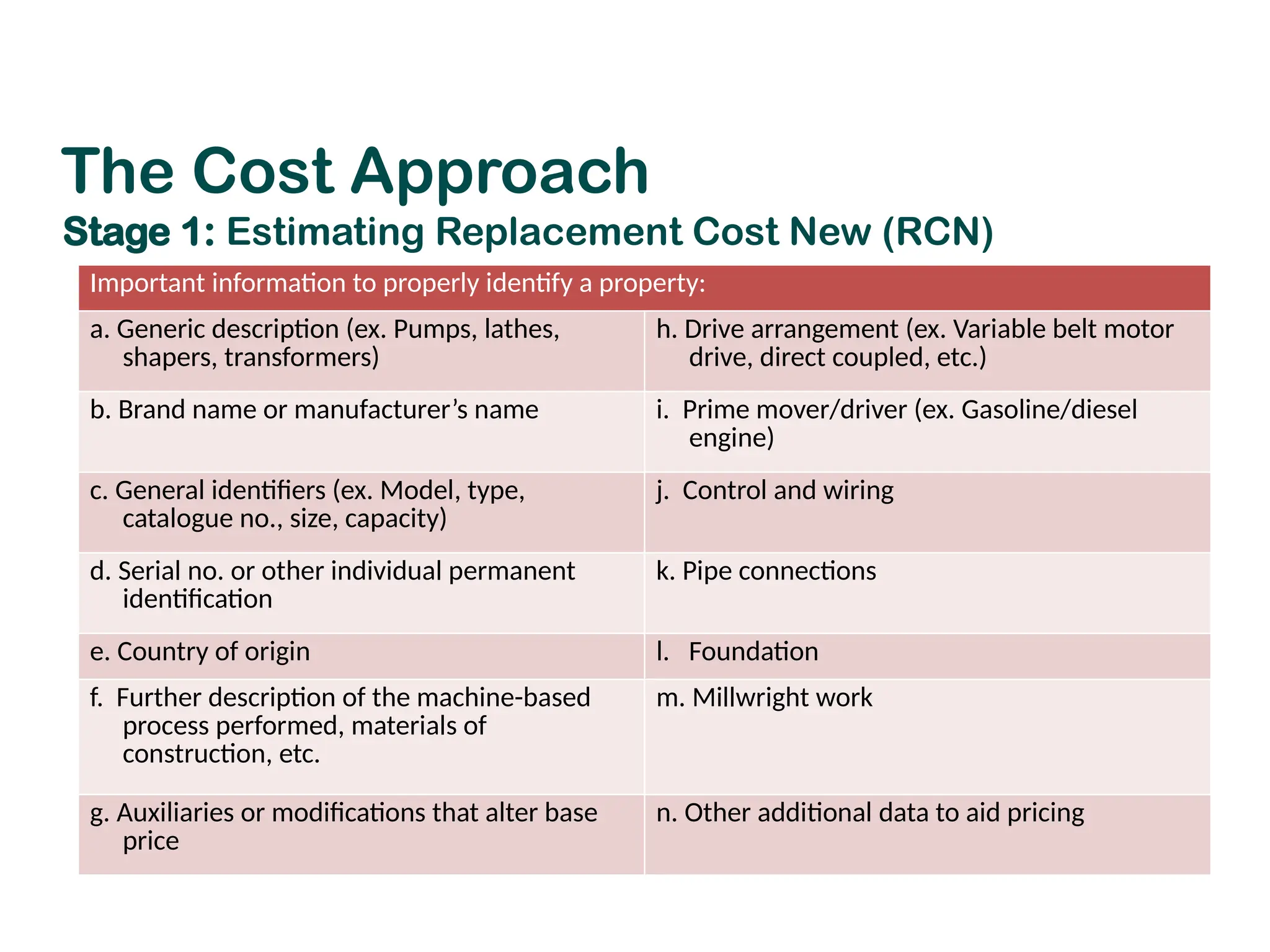
Important information toproperly identify a property:
a. Generic description (ex. Pumps, lathes,
shapers, transformers)
h. Drive arrangement (ex. Variable belt motor
drive, direct coupled, etc.)
b. Brand name or manufacturer’s name i. Prime mover/driver (ex. Gasoline/diesel
engine)
c. General identifiers (ex. Model, type,
catalogue no., size, capacity)
j. Control and wiring
d. Serial no. or other individual permanent
identification
k. Pipe connections
e. Country of origin l. Foundation
f. Further description of the machine-based
process performed, materials of
construction, etc.
m. Millwright work
g. Auxiliaries or modifications that alter base
price
n. Other additional data to aid pricing
The Cost Approach
Stage 1: Estimating Replacement Cost New (RCN)
167.
Techniques in Estimatingthe RCN
1. Re-pricing Technique
requires the valuer/appraiser to properly identify the items
being considered
establish the replacement cost new (RCN) of all items and
attachments
The Cost Approach
Stage 1: Estimating Replacement Cost New (RCN)
168.
Steps in usingthe Re-pricing Technique:
1. Establish an inventory of the property as of appraisal date
2. Gather adequate technical specifications of property items to be
re-priced for complete identification
3. Compile the basic price information or unit prices for each
property item from manufacturers, suppliers or dealers
4. Develop unit prices covering all elements of cost
5. Apply the unit prices to items that make up the machinery to
arrive at an indication of RCN
The Cost Approach
Stage 1: Estimating Replacement Cost New (RCN)
169.
NOTE: Valuation ofa multi-component production line
Requires many inputs
Involves considerable process and time in establishing
replacement and installation costs, especially if the machinery has
been customized, and the suppliers have difficulty in providing
current information
Repricing technique requires a specialized skill, considerable
patience, and may be considered impractical for SMV and rating
purposes, given the current level of LGU resources.
The Cost Approach
Stage 1: Estimating Replacement Cost New (RCN)
170.
2. Indexing Technique
Assumes that a new item of a particular type would now
cost the same as the original but multiplied by a factor to
account for inflation, changes in cost of materials and
labor, etc.
Can be used if original cost and date of acquisition of
property are known.
The Cost Approach
Stage 1: Estimating Replacement Cost New (RCN)
171.
2. Indexing Technique
Complication arises when a machine is superseded by a
more efficient machine that costs less than the particular
machine.
• The cost of the replacement machine is considered
for depreciation
For imported machinery, the RCN has to be adjusted for
currency fluctuations by dividing the exchange rate at
date of valuation by the exchange rate at date of
acquisition
The Cost Approach
Stage 1: Estimating Replacement Cost New (RCN)
172.
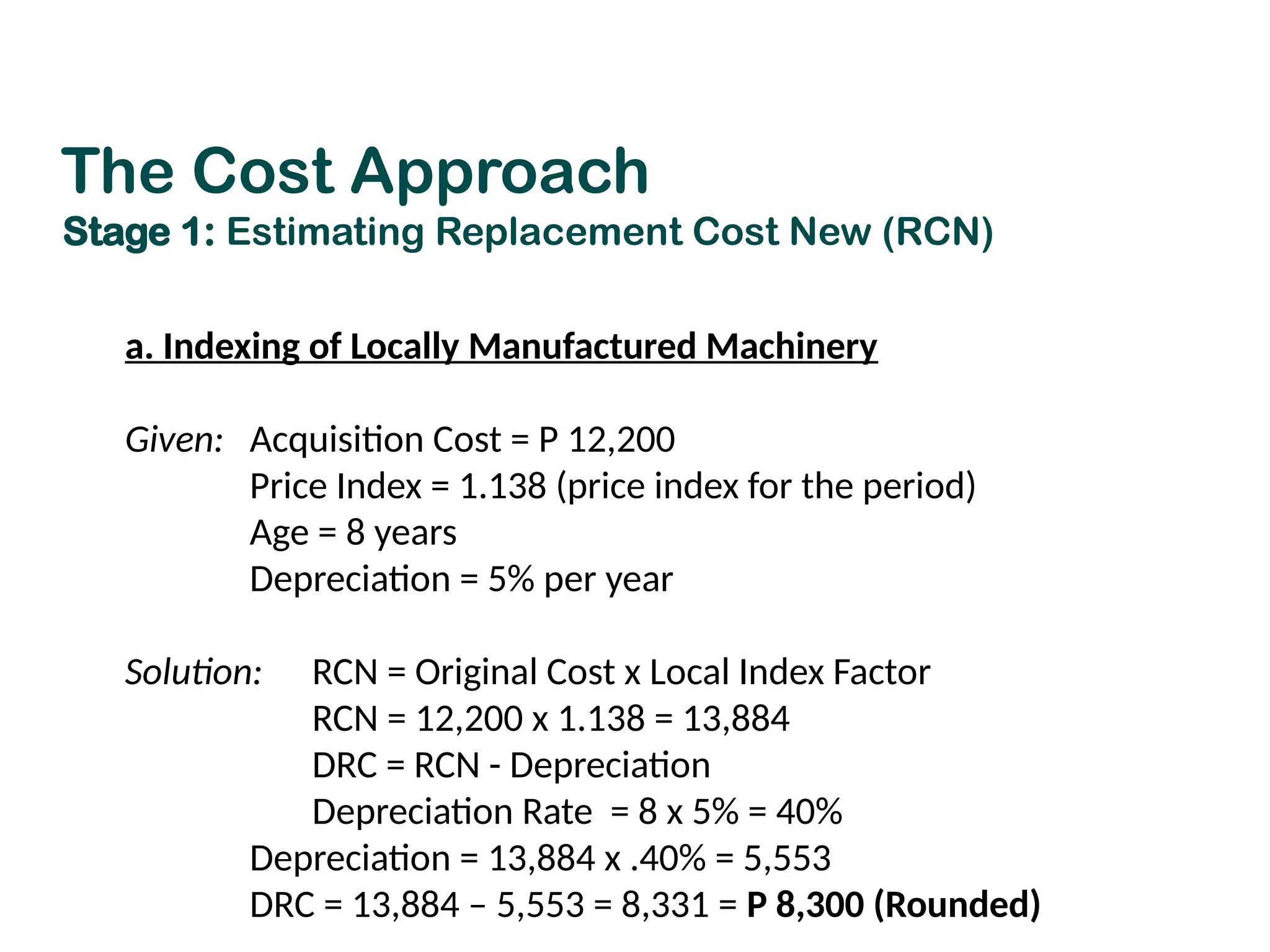
a. Indexing ofLocally Manufactured Machinery
Given: Acquisition Cost = P 12,200
Price Index = 1.138 (price index for the period)
Age = 8 years
Depreciation = 5% per year
Solution: RCN = Original Cost x Local Index Factor
RCN = 12,200 x 1.138 = 13,884
DRC = RCN - Depreciation
Depreciation Rate = 8 x 5% = 40%
Depreciation = 13,884 x .40% = 5,553
DRC = 13,884 – 5,553 = 8,331 = P 8,300 (Rounded)
The Cost Approach
Stage 1: Estimating Replacement Cost New (RCN)
173.
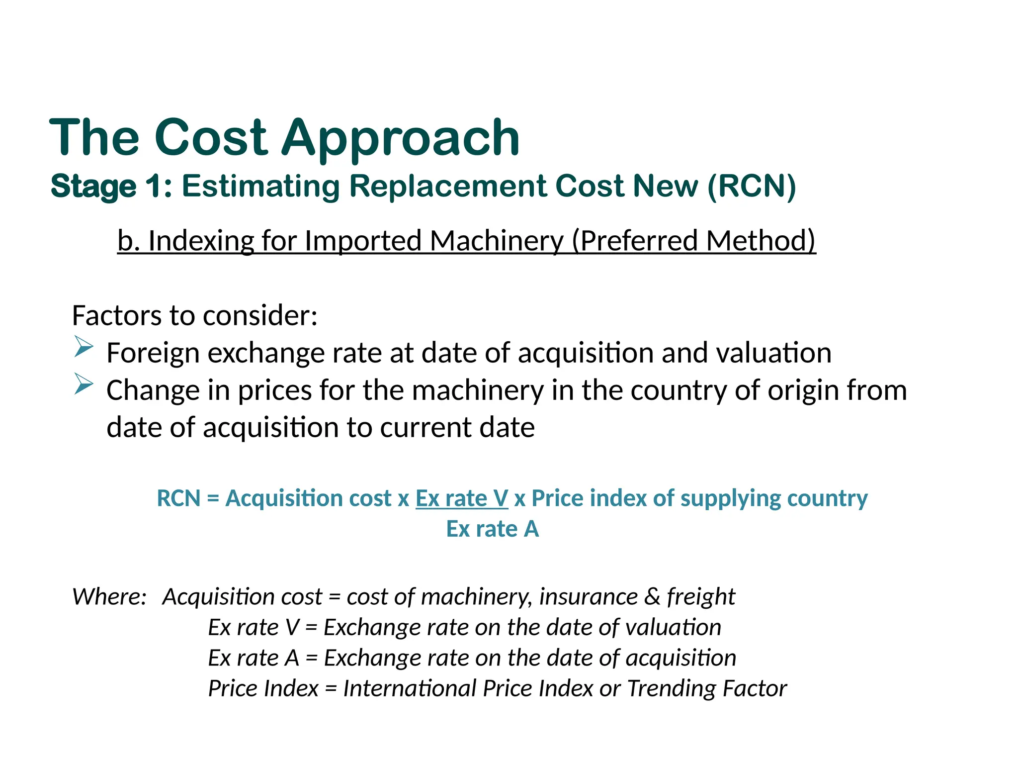
b. Indexing forImported Machinery (Preferred Method)
Factors to consider:
Foreign exchange rate at date of acquisition and valuation
Change in prices for the machinery in the country of origin from
date of acquisition to current date
RCN = Acquisition cost x Ex rate V x Price index of supplying country
Ex rate A
Where: Acquisition cost = cost of machinery, insurance & freight
Ex rate V = Exchange rate on the date of valuation
Ex rate A = Exchange rate on the date of acquisition
Price Index = International Price Index or Trending Factor
The Cost Approach
Stage 1: Estimating Replacement Cost New (RCN)
174.
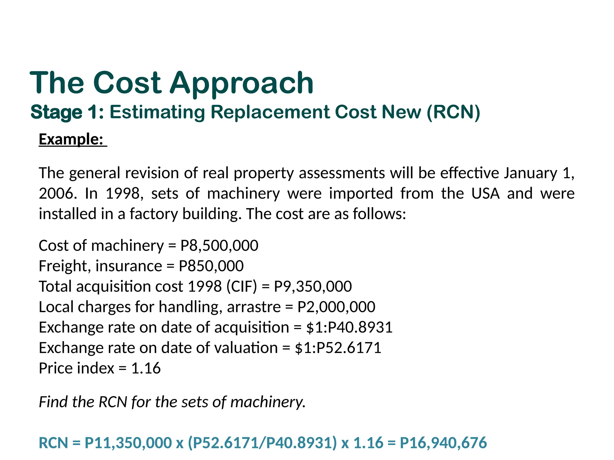
Example:
The general revisionof real property assessments will be effective January 1,
2006. In 1998, sets of machinery were imported from the USA and were
installed in a factory building. The cost are as follows:
Cost of machinery = P8,500,000
Freight, insurance = P850,000
Total acquisition cost 1998 (CIF) = P9,350,000
Local charges for handling, arrastre = P2,000,000
Exchange rate on date of acquisition = $1:P40.8931
Exchange rate on date of valuation = $1:P52.6171
Price index = 1.16
Find the RCN for the sets of machinery.
RCN = P11,350,000 x (P52.6171/P40.8931) x 1.16 = P16,940,676
The Cost Approach
Stage 1: Estimating Replacement Cost New (RCN)
175.
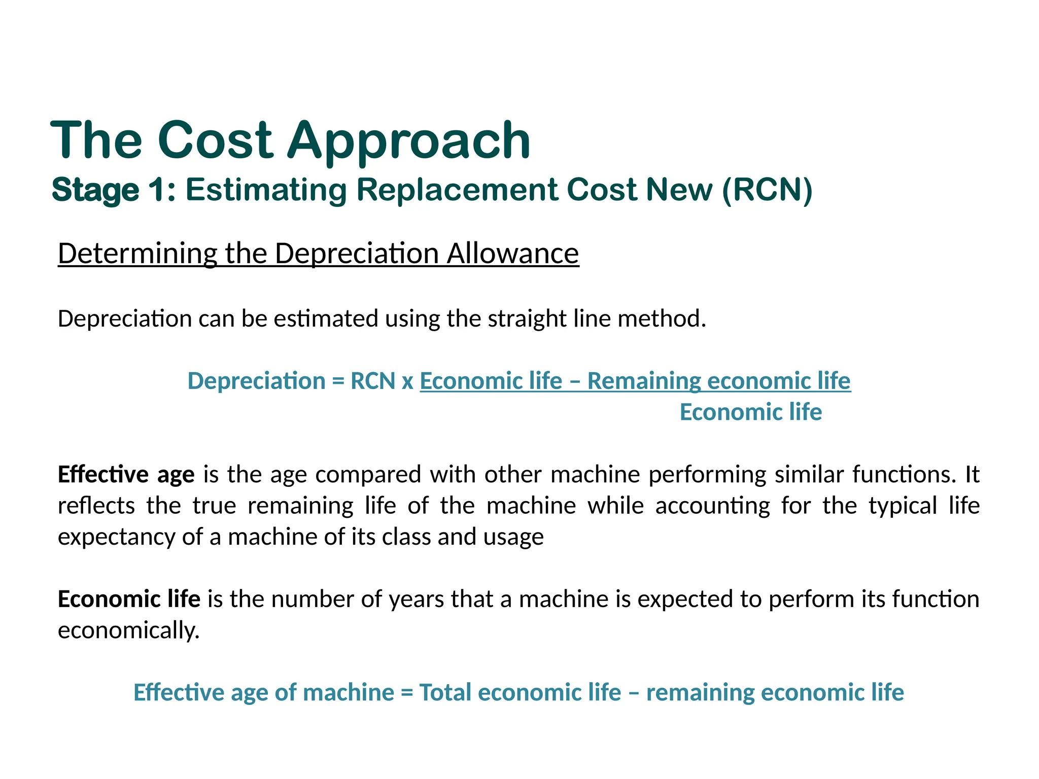
Determining the DepreciationAllowance
Depreciation can be estimated using the straight line method.
Depreciation = RCN x Economic life – Remaining economic life
Economic life
Effective age is the age compared with other machine performing similar functions. It
reflects the true remaining life of the machine while accounting for the typical life
expectancy of a machine of its class and usage
Economic life is the number of years that a machine is expected to perform its function
economically.
Effective age of machine = Total economic life – remaining economic life
The Cost Approach
Stage 1: Estimating Replacement Cost New (RCN)
176.
It is necessaryto verify whether the physical condition of the
machine coincides with the Sworn Statement.
Particularly for larger-scale enterprises with high-value
machinery
Verification aims to check the completeness of the
information on the Sworn Statement and check whether the
economic and remaining economic lives are realistic.
The Cost Approach
Stage 2: Verification
177.
If the declaredmarket value is still questionable, the value
may be checked with the manufacturer, supplier, dealer,
banks or other government agencies such as BIR, BOC,
SEC, etc.
Estimate the direct and indirect costs if data are not
available.
An ocular inspection should be conducted prior to
valuation.
The Cost Approach
Stage 2: Verification
178.
General Procedure inConducting an Ocular Inspection:
Discuss the Sworn Statement entries with management and
accountant or financial manager and verify the original
acquisition cost, including all direct and indirect costs, and
the condition of the machine when purchased.
Inspect the machinery to verify physical existence of the
property and identify entries, and confirm specifications and
other accessories.
Interview the plant and maintenance engineer and machine
operators to ascertain the service/maintenance history,
general condition and degree of obsolescence and expected
remaining economic life.
The Cost Approach
Stage 2: Verification
179.
Valuation of OtherInfrastructure
Rail tracks, wharves, piers, pipelines, etc., and electric
poles, cell sites and any related building or machine
rooms are treated as structures
Transmission machinery, equipment, satellite dishes,
etc. and associated cables are treated as machinery.
• These structures and machinery are valued using
Depreciated Replacement Cost.
• Valuation methodology to be used is the cost or sales
approach.
180.
Issues that willaffect the quality of the valuation
conclusions:
1. The reliability of data supplied by owners in the Sworn
Statement
2. The lack of power to compel owners to supply full and reliable
data
3. Machinery acquired as second-hand may be shown as ‘new’
acquisition
4. Difficulty in reconciling multiple entries listed over numerous
years, particularly the treatment of maintenance and repair
costs, with physical assets on the ground
5. The need for physical inspections to verify data supplied by
owners
General Valuation Issues
181.
6. Availability offinancial resources and the technical ability of
individuals undertaking verification
7. Reliance on a central valuation unit to supply annually
approved data schedules to all assessors
8. The primary depreciation factor being established by age only,
with no reference to condition.
9. The provision of Section 225 of the LGC which requires a
maximum depreciation of 5% which may produce unrealistic
results for assets with short economic lives and is in conflict
with the principle of establishing market values.
General Valuation Issues
182.
11. The interpretation/definitionof taxable machinery.
12. Machinery no longer being subjected to RPT in many western
economies unlike the Philippines where machinery generates
significant revenues.
13. There is a general lack of suitable resources to undertake
physical inspections, record data and carry out Observed
Condition Method (as provided in the Machinery and
Equipment Code (RA 8495).
General Valuation Issues
WHY CONDUCT ATAX IMPACT STUDY?
1. To provide local government officials and
the public with information on:
• Projected Property Owners’ Tax Burden
• Potential LGU revenue
2. To provide basis for formulating tax policy
options
3. To help explain the rationale and impact of
revising the SMV
4. To promote transparency in the property
tax system
186.
TRUE or FALSE?
•Real Property Tax is strictly value driven
• An increase in the SMV automatically leads to
a proportionate increase in the RPT
187.
Misconceptions about SMVRevision and
Increase in RPT
The increase in real
property tax is strictly
value driven
The increase in the
SMV automatically
leads to a
proportionate
increase in the RPT
Real Property Tax
Atax imposed by provinces and cities on real
property such as land, buildings, machinery and
other improvements.
Annual ad valorem tax (basic RPT);
Additional levy for the Special Education Fund
(SEF); and
Others (idle land tax, special levy on lands
benefitted by public works projects, socialized
housing tax)
190.
Calculating the RealProperty Tax
Market
Value
Assessment
Level
Tax
Rate
Real Property
Tax
X
X =
Assessed Value
191.
Prescribed Assessment Levelsfor Land and RPT Rates
(Local Government Code)
ASSESSMENT LEVELS TAX RATES
Maximum of
Residential - 20% Basic RPT: Maximum of
Commercial - 50% For cities - 2%
Industrial - 50% For provinces - 1%
Agricultural - 40% SEF: Fixed rate of 1%
Mineral - 50% Idle land: 5%
Timberland - 20% Socialized housing 0.05%
The LGC prescribes the maximum levels and tax rate ceilings; LGUs
are authorized to lower the assessment levels and tax rates
through the enactment of an ordinance.
192.
Calculating the RPTUnder the Current and
New Market Value
Exercise 1:
Consider a 100 m2
residential land with a current market
value of P1,000/m2
(based on current SMV) and proposed
market value of P2,000/m2
. The LGU imposes the maximum
assessment level of 20% and tax rate of 2% (1% basic RPT and
1% SEF).
Calculate the current and proposed RPT; and the percent
RPT increase.
193.
What is theincrease in Real Property Tax (RPT) given
the increase in unit base market value at constant
assessment level and tax rate?
Given:
Lot Area = 100m2
Current Market Value (MV) = P1,000/m2
Proposed Market Value (MV) = P 2,000/m2
Current Assessment Level = 20%
Current Tax Rate = 2%
Solution:
Current RPT = 100m2
x P1,000/m2
x 20% x 2%
Current RPT = P 400
Proposed RPT = 100m2
x P2,000/m2
x 20% x 2%
Proposed RPT = P 800
% RPT Increase = 100%
194.
What are thepossible RPT Policy
Options?
Given the 100% increase in unit base market value at
the same assessment level and tax rate,
Identify possible real property tax options.
195.
Possible Tax Options
Option1: Reduce the assessment level to a
specified percentage
Option 2: Reduce the tax rate to a specified
percentage
Option 3: Combination of Options 1 and 2
196.
What is theAssessment Level (AL)?
Given:
% increase in RPT = 30%
Land Area = 100 m2
Current MV = P1,000/m2
Current A.L. = 20%
Proposed MV = P 2,000/m2
Current Tax Rate = 2%
Solution:
Current RPT = 100 x 1,000 x 20% x 2%
Current RPT = P 400
Proposed RPT @ 30% increase = P 400 x 1.3
Proposed RPT @ 30% increase = P 520
AL = 520/(100 x 2,000 x 2%)
AL = 0.13 or 13%
Option 1: Reduce the assessment level to a specified
percentage
197.
What is theTax Rate (TR)?
Given:
% increase in RPT = 30%
Land Area = 100 m2
Current MV = P 1,000/m2
Current A.L. = 20%
Proposed MV = P 2,000/m2
Current Tax Rate = 2%
Answer:
Current RPT = 100 x 1,000 x 20% x 2%
Current RPT = P 400
Proposed RPT @ 30% increase = P 400 x 1.3
Proposed RPT @ 30% increase = P 520
TR = 520/(100 x 2,000 x .2)
TR = 0.013 or 1.3%
Option 2: Reduce the tax rate to a specified percentage
198.
Given:
Land Area =100 m2
Current MV = P 1,000/m2
Proposed MV = P 2,000/m2
Current A.L. = 20%
Current Tax Rate = 2%
Current Option 1 Option 2
Assessment Level (%) 20 13 20
Tax Rate (%) 2 2 1.3
RPT (Php) 400 520 520
Possible RPT PolicyOptions
Option 1: Reduce the Tax Rate (e.g., from 1% to
0.75%)
Option 2: Reduce the assessment levels from 20%
to 10%
201.
Given:
Total Land Area= 10,000,000m2
Current Market Value (MV) = P1,000/m2
Proposed Market Value (MV) = P2,000/m2
Current Assessment Level = 20%
Current Tax Rate = 2%
Answer:
Current LGU Revenue
LGU Revenue = 10,000,000x 1,000 x 20% x 2%
LGU Revenue = P40,000,000
Potential LGU Revenue
LGU Revenue = 10,000,000x 2,000 x 20% x 2%
LGU Revenue = P80,000,000
What is the current and potential LGU Revenue?
202.
Given:
Total Land Area= 10,000,000m2
Current Market Value (MV) = P1,000/m2
Proposed Market Value (MV) = P2,000/m2
Current Assessment Level = 20%
Current Tax Rate = 2%
Answer:
Potential LGU Revenue at Current AL of 20%
LGU Revenue = 10,000,000x 2,000 x 20% x 2%
LGU Revenue = P80,000,000
Potential LGU Revenue with Assessment Level of 13%
LGU Revenue = 10,000,000x 2,000 x 13% x 2%
LGU Revenue = P52,000,000
What is the effect on the potential LGU revenue if the
assessment level is reduced from 20% to 13%?
203.
Given:
Total Land Area= 10,000,000m2
Old Market Value (MV) = P1,000/m2
New Market Value (MV) = P2,000/m2
Current Assessment Level = 20%
Current Tax Rate = 2%
Answer:
Potential LGU Revenue at Current Tax Rate of 2%
LGU Revenue = 10,000,000x 2,000 x 20% x 2%
LGU Revenue = P80,000,000
Potential LGU Revenue with Tax Rate of 1.3%
LGU Revenue = 10,000,000x 2,000 x 20% x 1.3%
LGU Revenue = P52,000,000
What is the effect on the potential LGU revenue if the tax
rate is reduced from 2% to 1.3%?
204.
Current
MV
Using
Proposed MV
Option 1Option 2
Assessment Level (%) 20 20 13 20
Tax Rate (%) 2 2 2 1.3
Potential Revenue 40M 80M 52M 52M
Summary of Potential LGU Revenue Using
Different Tax Options
• Assigns variousvalues for different
locations and property classifications
• Have varying rates of increase in values
from the previous SMV
• Re-classified land parcels will have a range
of value increases
Proposed Schedule of Market Values
208.
1. List ofTax Exempt and Non-Exempt RPUs
a. Property identifiers – PIN, TDN, name and address of
owner, etc.
b. Property details – land area, floor area, property
classification, taxability, actual use, building type,
building condition, etc.
c. Assessment levels – generally vary by actual use
d. Tax rate – only 1 tax rate is adopted by LGUs but others
use differentiated tax rates for land, buildings and
machinery
e. RPT collectible – amount to be paid by taxpayers
Data Requirements in Formulating Tax Options:
209.
SN
# Tax Dec# Barangay
Property
Owner
Property
Type
Taxa-
bility
Property
Sub-
Class Area
Unit
Value
(SMV)
Market
Value
Adjust-
ments
Adjusted
MV AL
Assessed
Value Tax Rate
RPT
Collectible
1 2001-11-
0473-1
Abella Santos,
Ramona
Land T R1 250 200 50,000 - 50,000 20% 10,000 2% 200
2 2001-11-
0123-3
Abella Sese,
Pura
Land T R1 100 200 20,000 - 20,000 20% 4,000 2% 80
3 2001-11-
0473-1
Abella Torres,
Abad
Land T R1 230 200 46,000 (4,600) 41,400 20% 8.280 2% 166
4 2001-11-
14473-1
Abella Villanuev
a, oniaT
Land T R1 140 200 28,000 - 28,000 20% 5,600 2% 112
5 2001-11-
0473-1
Abella Santos,
Perla
Land T R1 120 200 24,000 2,400 26,400 20% 5,280 2% 106
6 2001-
1110473-1
Abella Senseng,
wilfredo
Land T R2 120 150 18,000 - 18,000 20% 3,600 2% 72
7 2001-12-
21473-1
Abella Rosales,
Juan
Land T R2 120 150 18,000 - 18,000 20% 3,600 2% 72
8 2001-12-
0473-1
Abella Rosales,
john
Land T R2 100 150 15,000 - 15,000 20% 3,000 2% 60
9 2001-12-
0473-1
Abella Bautista,
Feliciano
Land T R2 300 150 45,000 - 45,000 20% 9,000 2% 180
10 2001-122-
0473-1
Abella Reyes,
Nick
Land T R2 120 150 18,000 - 18,000 20% 3,600 2% 72
11 2001-31-
0473-1
Abella Nicolas,
Pedro
Land T R2 150 150 22,500 - 22,500 20% 4,500 2% 90
12 2001-
1110473-1
Abella Nicolas,
Mario
Land T R2 60 150 9,000 - 9,000 20% 1,800 2% 36
List of Tax Exempt and Non-Exempt RPUs
210.
2. Current andProposed SMV
Provides information on the current and
proposed property sub-classification, and
current and proposed unit values along different
streets/barangay in a city or municipality within
a province
Data Requirements in Formulating Tax Options:
211.
STREET/
SUBDIVISION
VICINITY
CURRENT SMV PROPOSEDSMV
CURRENT
BASE VALUE
SUB CLASS
PROPOSED
BASE VALUE
SUB CLASS
ABELLA 001
Abella Street
Gen. Luna St. J. Hernandez
Ave.
300 C-1 2,500 C-2
J. Hernandez Ave. - 1st
100m.
250 C-2 2,000 C-3
after 100m - Cnr Felix Plazo
St.
150 C-5 1,500 C-4
Cnr F. Plazo St.-Naga 200 R-1 2,000 R-1
Bayawas Street Abella Street-Looban 8 200 R-1 2,000 R-1
Felix Plazo Street
Abella St.- Igualdad
Boundary
200 R-1 2,000 R-1
All inner lots 150 R-3 1,000 R-5
J. Hernandez Ave. Prieto St.-P. Burgos St. 300 C-1 2,500 C-2
General Luna St Prieto St.-P. Burgos St. 300 C-1 3,000 C-1
P. Burgos Street Gen. Luna St.-J. Hernandez 300 C-1 3,000 C-1
Prieto Street
J. Hernandez St.-Gen. Luna
St.
250 I-1 1,500 I-1
BISALA 250 I-1 1,500 I-1
All Blighted Areas 100 R-5 500 R-8
Sample of Current & Proposed SMV
212.
Step 1: Calculatethe current & new RPT for all taxable land parcels
from the List of Tax Exempt & Non-Exempt RPUs
Step 2: Calculate the incremental RPT (tax impact) and % increase in the
tax due
Incremental RPT = Proposed (New) RPT – Current RPT
% increase = Incremental RPT x100
Current RPT
Steps in Calculating the Tax Impact of the
Proposed SMV:
213.
Step 3: Analyzethe tax impact of the new MV on all land parcels (or
sample land parcels)
a. Examine land parcels that will have lower RPT
b. Examine land parcels that will have higher RPT and then
determine the lowest, average and highest increase in RPT
c. Examine re-classified land parcels and determine the extent of
the increase in RPT
d. Examine land parcels that will be heavily affected by the
increase in RPT
Steps in Calculating the Tax Impact of the
Proposed SMV:
214.
Tax Impact Calculationof Sample Land Parcels in the Assessment Roll
Data from the List of Tax
Exempt & Non-Tax Exempt
RPUs
Data from Current &
Proposed SMV Computed Data
215.
Example: Consider thefollowing 4 sample land parcels
from the Assessment Roll:
Lot #1 – a 100 m2
R1 land with current market value of
P200/m2
and proposed market value of P2,000/m2
Lot #2 – a 100 m2
C1 land with current market value of
P300/m2
and proposed market value of P3,000/m2
Lot #3 – a 500 m2
I1 land with current market value of P250/m2
and proposed market value of P1,500/m2
Lot #4 – a 1 hectare RL1 land with current market value of
P40,300/ha and proposed market value of P200,000/ha
Calculating the Tax Impact of the Proposed SMV:
216.
Solution: Increase inRPT (Basic & SEF) Under the
Proposed SMV
Analysis:
• The increase in RPT ranges from 396% to 900%.
• The additional RPT to be paid by the taxpayers vary from P800 to P7,500.
• Increasing the current RPT by four to nine times will be too excessive for the
taxpayers.
• It is in this regard that certain tax policy adjustments should be considered.
Property
Class
Land
Area
Current
MV New MV
Total MV
based on
Current
MV
Total MV
based on
New MV AL (%)
Total AV
based on
Current
MV
Total AV
based on
New MV
TR
(%)
Current
RPT
New
RPT
Tax
Impact % Inc.
(a) (b) (c) (d) (e=bxc) (f=bxd) (g) (h=exg) (i=fxg) (j) (k=hxj) (l=ixj) (m=l-k) (n=m/
kx100)
R1 100m2
200 2,000 20,000 200,000 20 4,000 40,000 2 80 800 720 900
C1 100m2
300 3,000 30,000 300,000 50 15,000 150,000 2 300 3,000 2,700 900
I1 500m2
250 1,500 125,000 750,000 50 62,500 375,000 2 1,250 7,500 6,250 500
RL-1st 1ha. 40,300 200,000 40,300 200,000 40 16,120 80,000 2 322 1,600 1,278 396
Guidelines in FormulatingTax Options
1. Avoid reducing (or minimize the reduction)
the RPT. Target some % increase in the tax
over the previous individual tax bill.
2. Avoid (or minimize the impact of the increase)
significant increases in the initial RPT.
3. Ensure that the RPT increases in absolute
amounts are acceptable and affordable to all
taxpayers.
219.
Step 1: Identifypossible tax options.
Step 2: Calculate the current and proposed RPT for all
taxable land parcels from the Assessment Roll
under each tax option.
Step 3: Calculate the incremental RPT and percent
increase in tax under each tax option.
Step 4: Analyze and compare the tax impact of various
tax options and initially choose the best option.
Steps in Calculating the Tax Impact of Tax
Options:
220.
Example: Increase inRPT (Basic and SEF) Under Option 1
Analysis: Option 1 (reduce assessment level by 70%)
• The increase in RPT ranges from 49% to 200% or P158 to P1,000.
• Riceland has the least amount of increase whereas industrial land has the highest.
• Percentage-wise, residential and commercial lands, have the highest rate increase.
Property
Class
Land
Area SMV
New
MV
Total MV
Based on
SMV
Total MV
Based on
New MV
Cur-
rent
AL
(%)
Opti
on 1
AL
(%)
Total AV
Based
on SMV
Total AV
Based on
Option 1
TR
(%)
Current
RPT
RPT
Under
Option
1
Tax
Impact % Inc.
(a) (b) (c ) (d)
e
= b x c (f=b x d) (g) (h)
i
= e x g (j=f x h) (k)
l
=i x k
m
=j x k
n
=m - l
o=n/l
x100
R1
100
m2 200 2,000 20,000 200,000 20 6 4,000 12,000 2 80 240 160 200
C1
100
m2 300 3,000 30,000 300,000 50 15 15,000 45,000 2 300 900 600 200
I1
500
m2 250 1,500 125,000 750,000 50 15 62,500 112,500 2 1,250 2,250 1000 80
RL-1st 1 ha. 40300 200,000 40,300 200,000 40 12 16,120 24,000 2 322 480 158 49
221.
Example: Increase inRPT (Basic & SEF) Under Option 2
Analysis: Under Option 2 (reduce tax rate from 2% to 1%)
• The increase in RPT ranges from 148% to 400% or P400 to P3,750.
• Although the basic RPT rate can be reduced, the SEF rate is fixed at 1%.
• Reducing the tax rate from 2% to 1% means that any proceeds from RPT will go to the SEF.
Property
Sub-
Class
Land
Area SMV
New
MV
Total
MV
Based
on SMV
Total MV
Based on
New MV
AL
(%)
Total AV
Based
on SMV
Total AV
Based on
New MV
Current
Tax Rate
(%)
Option
2
TR (%)
Current
RPT
RPT
Under
Option
2
Tax
Impact % Inc.
(a) (b) (c ) (d)
e
= b x c
(f=b x d) (g)
(h=e x
g)
(i=f x g) (j) (k)
l
= h x j
m
= i x k
(n=m - l)
o
=n/l
x100
R1
100
m2 200 2,000 20,000 200,000 20 4,000 40,000 2 1% 80 400 320 400
C1
100
m2 300 3,000 30,000 300,000 50 15,000 150,000 2 1% 300 1,500 1,200 400
I1
500
m2 250 1,500 125,000 750,000 50 62,500 375,000 2 1% 1,250 3,750 2,500 200
RL-1st 1 ha. 40,300 200,000 40,300 200,000 40 16,120 80,000 2 1% 322 800 478 148
222.
Example: Increase inRPT (Basic & SEF) Under Option 3
Analysis: Under Option 3 (reduce AL by 60% & TR from 2% to 1.5%)
• Reduction of the tax rate from 2% to 1.5% means that the SEF tax rate is maintained at 1% while
the basic RPT rate is reduced from 1% to 0.5%.
• Although this is feasible, consider that about two-thirds of the increase in the RPT will go to the
SEF whereas a third will go to the General Fund.
Proper
ty
Class
Land
Area SMV
New
MV
Total MV
Based
on SMV
Total MV
Based
on New
MV
Cur-
rent
AL
(%)
Op-
tion
3 AL
(%)
Total
AV
Based
on SMV
Total AV
Based
on
Option 3
Curr
entT
R
(%)
Op-
tion
3 TR
(%)
Cur-
rent
RPT
RPT
Under
Op-
tion 3
Tax
Imp-
act % Inc.
(a) (b) (c ) (d)
e
= b x c
(f=b x d) (g) (h)
i
= e x g
(j=f x h) (k)
l
=i x k
(m)
n
=j x l
o
=n-m
p
=o/m
x100
R1
100
m2 200 2,000 20,000 200,000 20 8 4,000 16,000 2 1.5 80 240 160 200
C1
100
m2 300 3,000 30,000 300,000 50 20 15,000 60,000 2 1.5 300 900 600 200
I1
500
m2 250 1,500 125,000 750,000 50 20 62,500 150,000 2 1.5 1,250 2,250 1,000 80
RL -
1st
1 ha. 40,300 200k 40,300 200,000 40 16 16,120 32,000 2 1.5 322 480 158 49
223
223.
SUMMARY: Increase inRPT (Basic and SEF) Under Various
Tax Options
Property
Class
Land
Area
SMV
Proposed
MV
Assess -
ment
Level
(%)
Tax
Rate
(%)
Current
RPT
RPT
Under
Proposed
MV
Option
1
Option
2
Option
3
R1
100
m2 200 2,000 20 2 80 800 240 400 240
C1
100
m2 300 3,000 50 2 300 3,000 900 1,500 900
I1
500
m2 250 1,500 50 2 1,250 7,500 2,250 3,750 2,250
RL -1st 1 ha. 40,300 200,000 40 2 322 1,600 480 800 480
224
Computing the PotentialLGU Revenue from
the Proposed SMV:
Step 1: Summarize the potential RPT under the current SMV and
under the proposed SMV for all taxable land parcels by
property classification or by barangay.
Step 2: Calculate the incremental LGU revenue by subtracting the
current LGU revenue from the potential LGU revenue.
Step 3: Adjust the revenue impact considering the following:
a. Compliance Ratio/Collection Efficiency
b. Discounts
c. Fines and penalties
d. Tax incentives, if any
Estimated Total RevenueImpact of the
Proposed SMV
Property
Type
RPT Collectible
Coll.
Eff.
(%)
RPT Revenue @ Current Collection
Efficiency Current
RPT
Revenue
Projected
Total
Revenue
Impact
Less:
Dis-
count
Plus:
Fines &
Penal-
ties
Net
Incre-
mental
Rev
Current
SMV
Proposed
SMV
Current
SMV
Proposed
SMV
Revenue
Impact
%
Increase
TOTAL 105 285 53 56 154 98 75 112 196 20 14 190
Res’l 53 129 45 24 58 34 42 48 68 7 5 64
Comm’l 8 23 60 5 14 9 80 10 18 2 1 18
Ind’l 38 115 65 25 75 50 100 50 100 10 7 97
Agric’l 5 17.5 40 2 7 5 150 4 10 1 1 11
228.
Calculating the PotentialLGU Revenue from
Various Tax Options
Step 1: Calculate the revenue impact for each tax option.
Step 2: Summarize the revenue impact of the various tax
options by property classification or by barangay.
Step 3: Choose the best tax option considering the budgetary
requirements of the LGU and the tax impact on
individual taxpayers.
229.
Calculating the PotentialLGU Revenue
from Various Tax Options
Property Type
Estimated Incremental Revenue at Current Coll. Efficiency
Proposed SMV Option 1 Option 2 Option 3
TOTAL 190.16 57.05 28.52 57.05
Residential 63.43 19.03 9.515 19.03
Commercial 18.39 5.52 2.76 5.52
Industrial 97.3 29.19 14.60 29.19
Agricultural 11.06 3.32 1.66 3.32
Revenue Impact Calculation Summary (in million P)
230
230.
REFERENCE
National Tax ResearchCenter. A Guidebook on the Conduct of a Tax
Impact Study of Proposed Schedule of Market Values in Local
Governments.

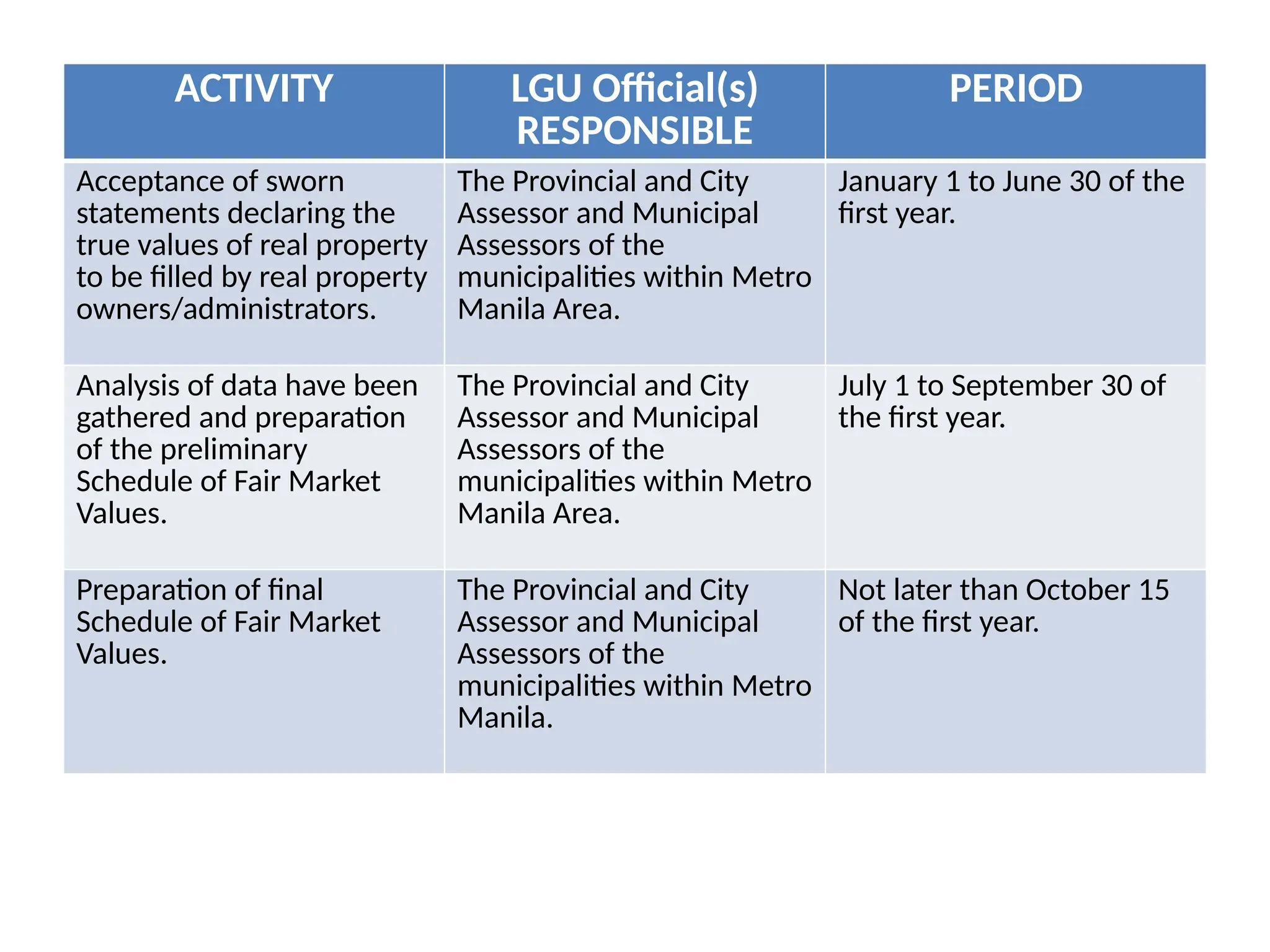
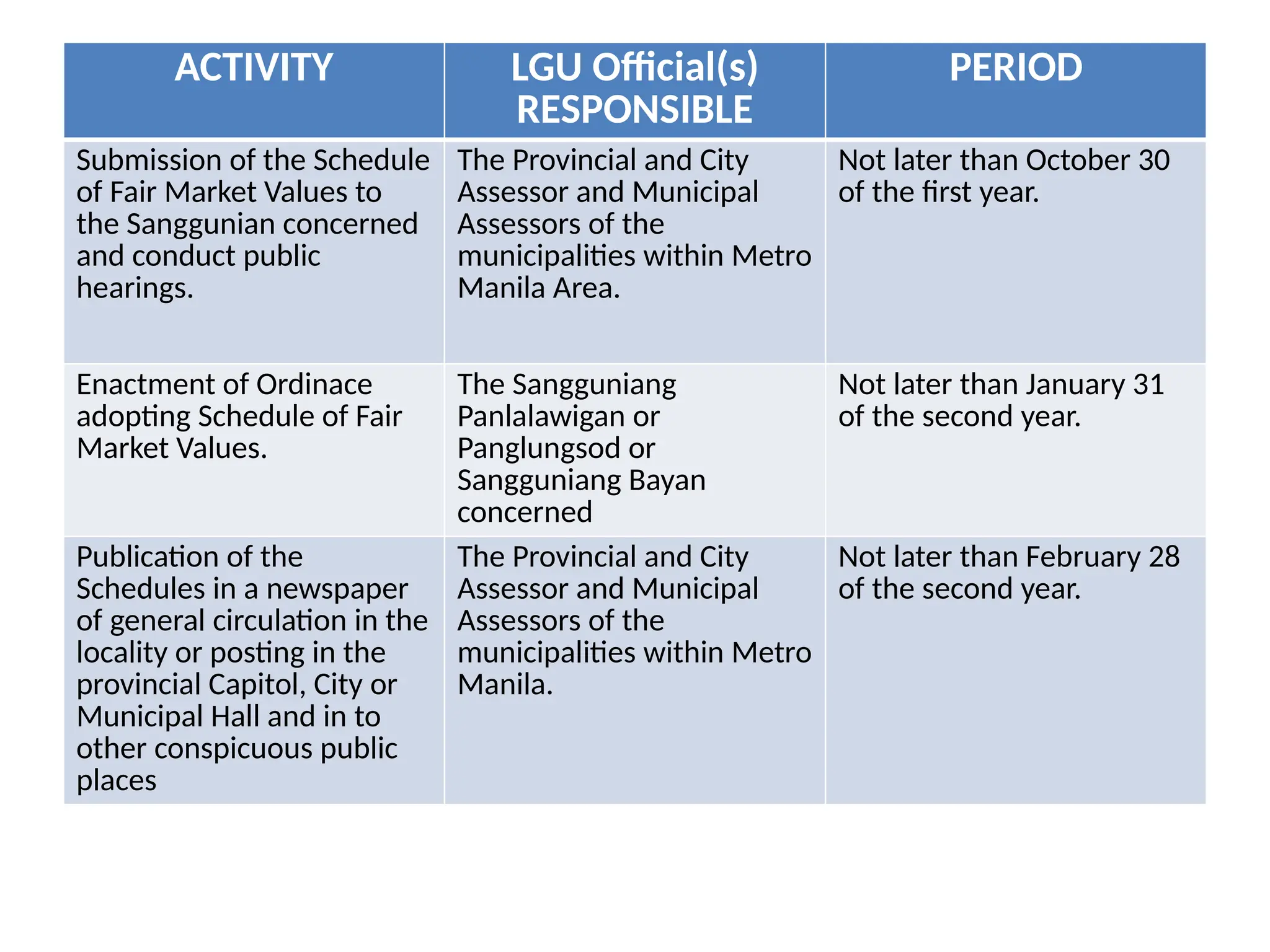
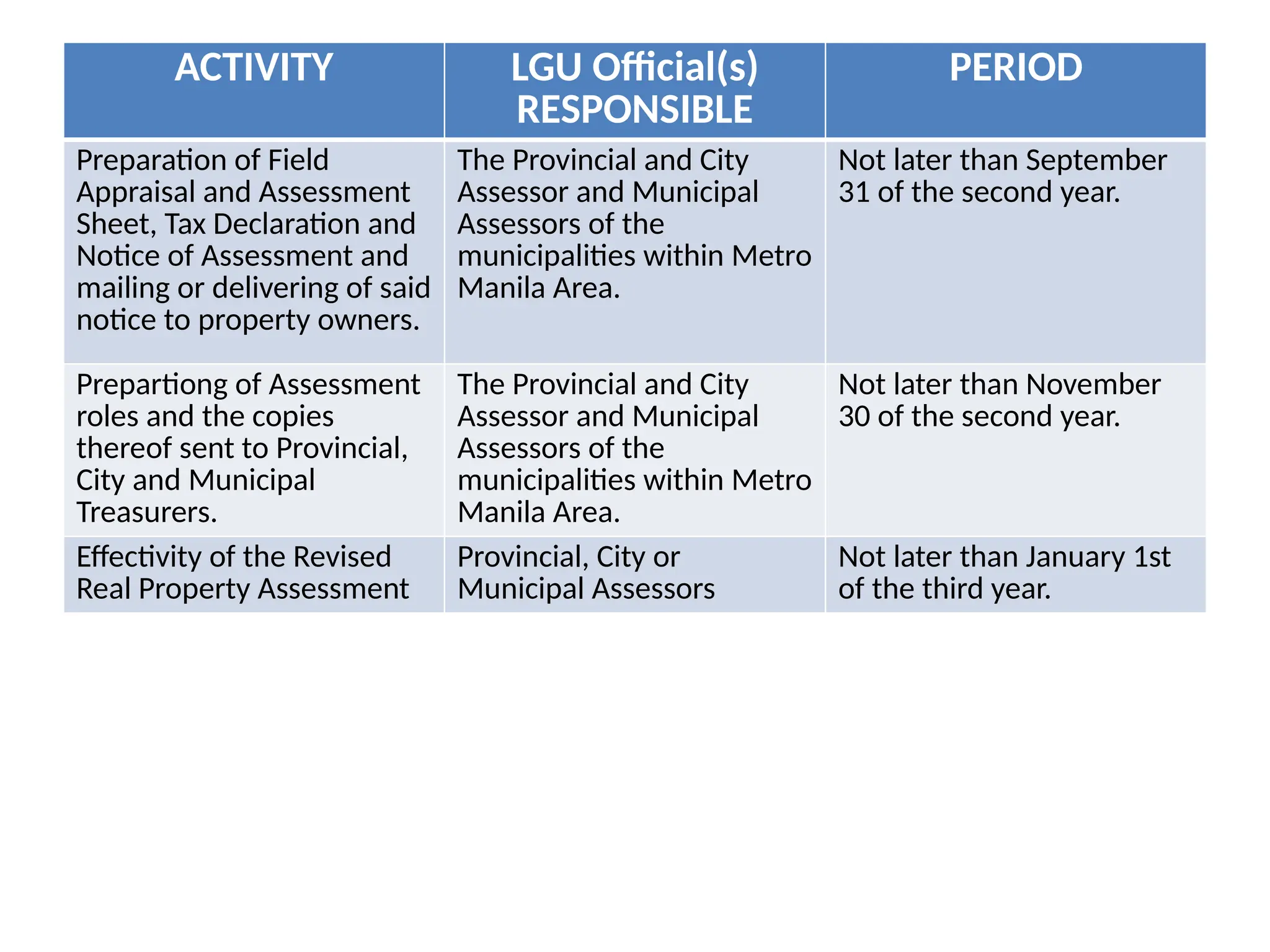

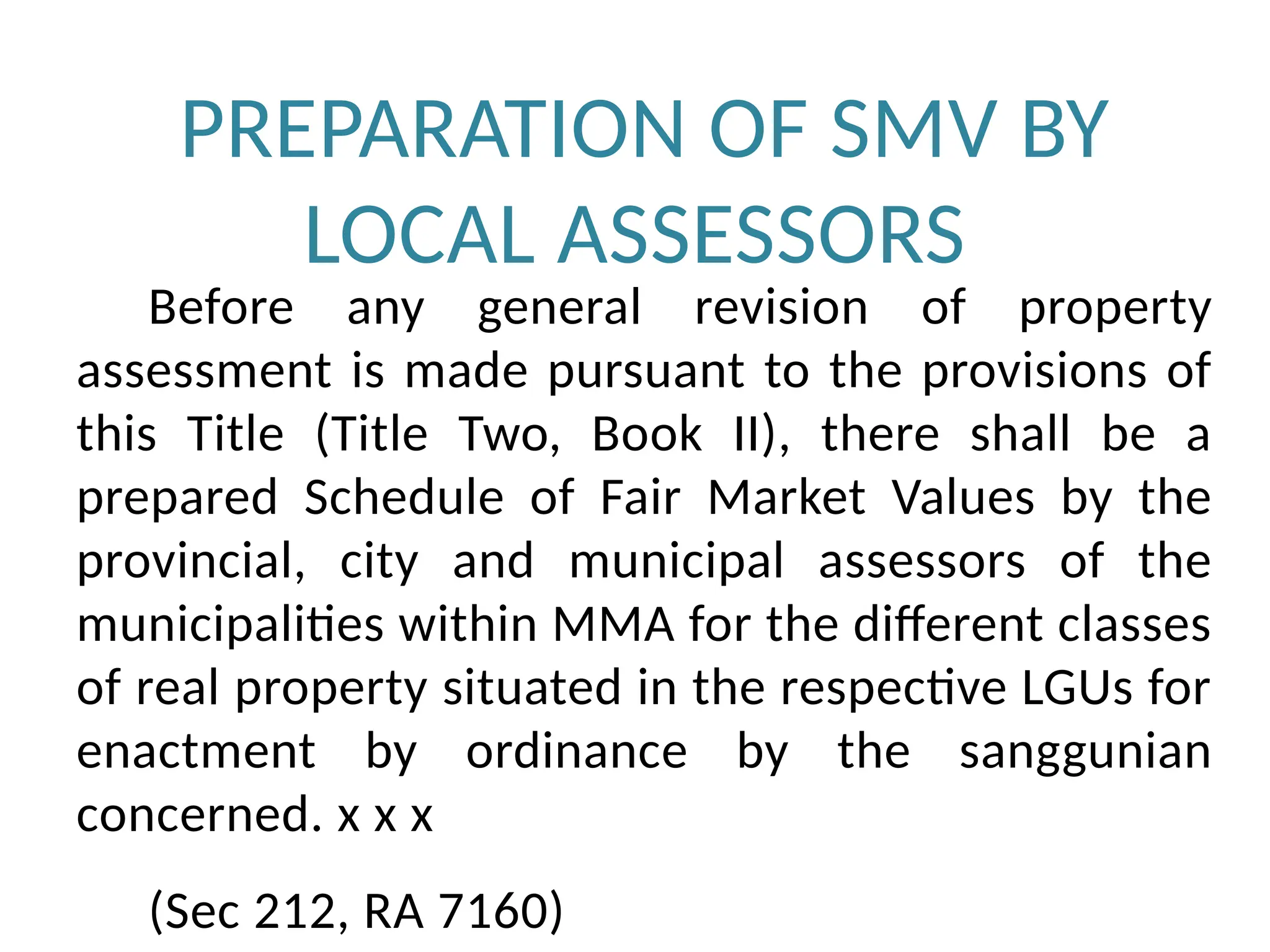

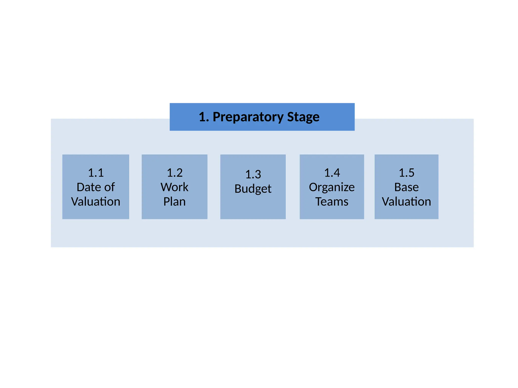
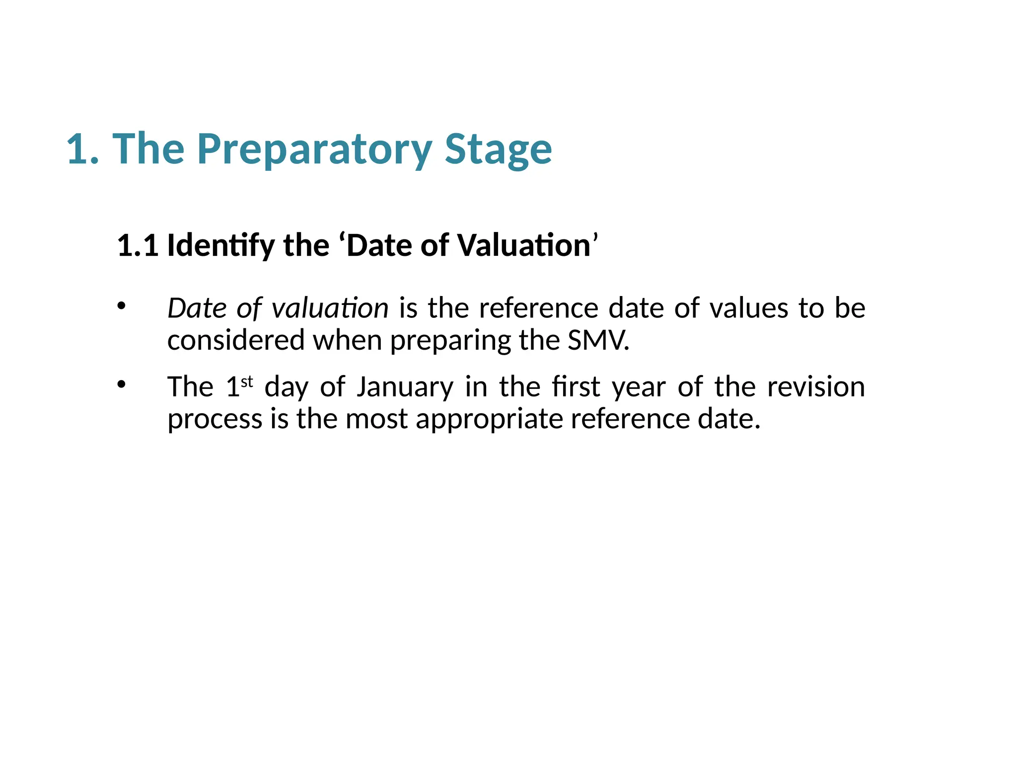


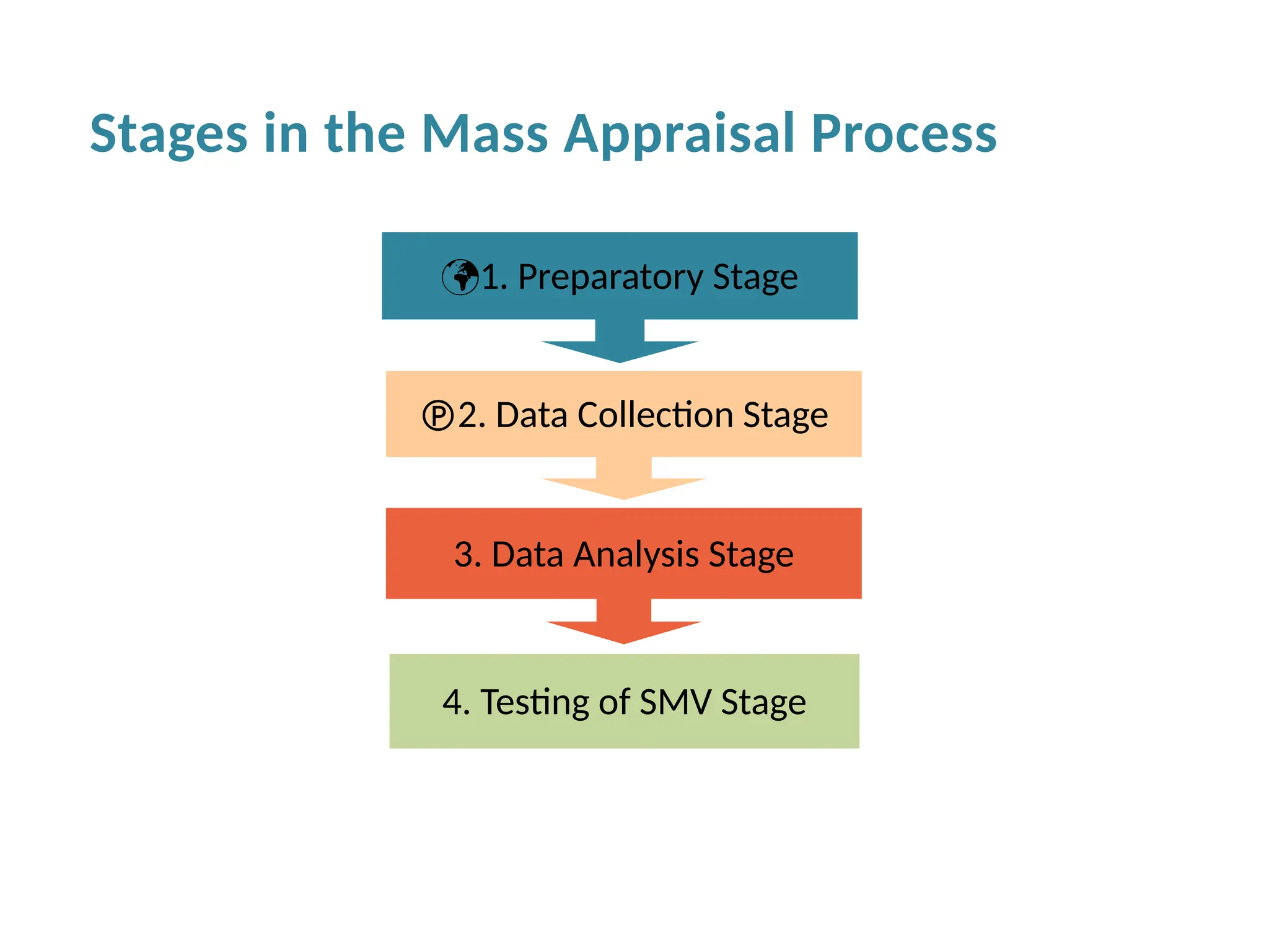
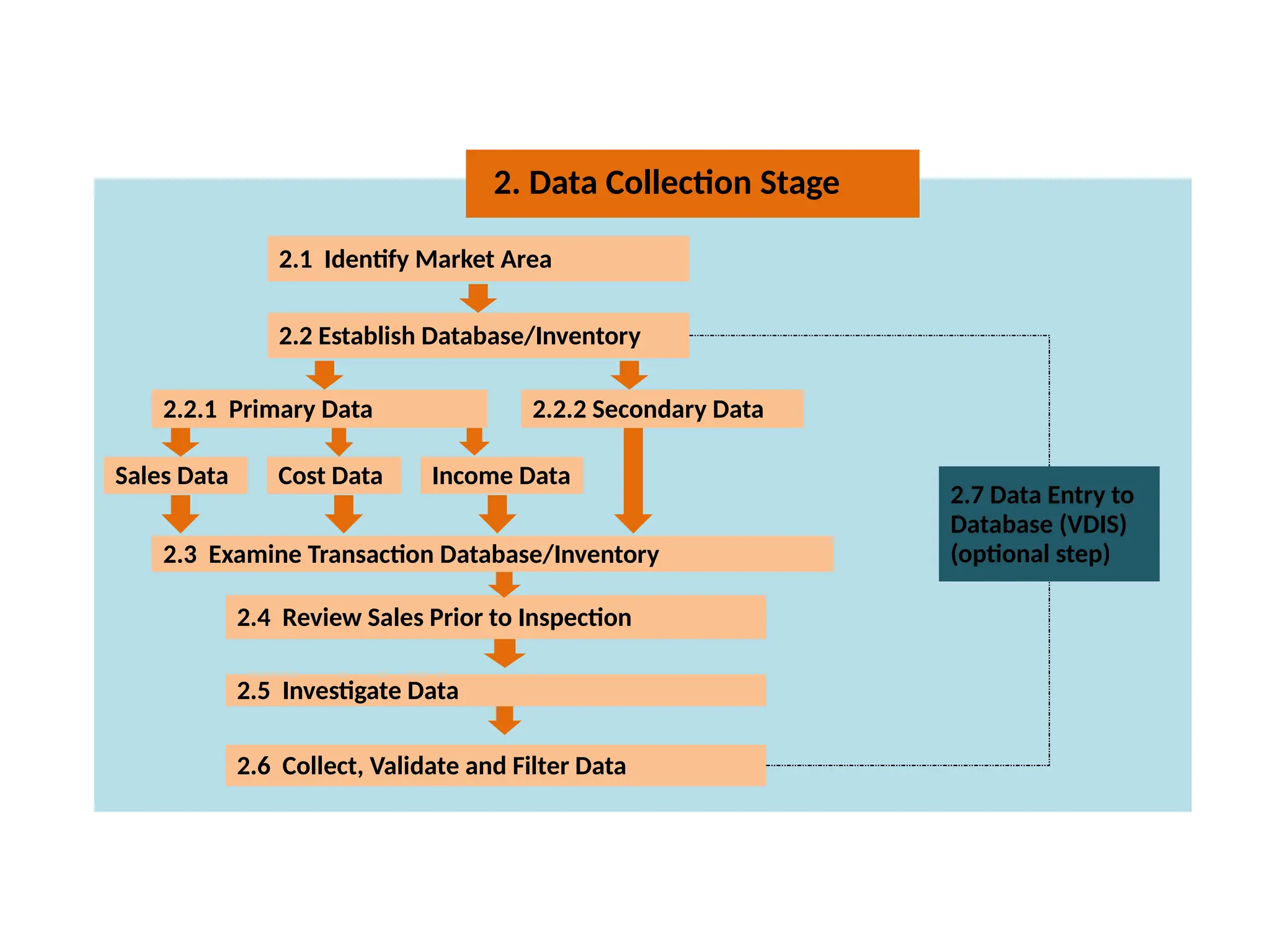
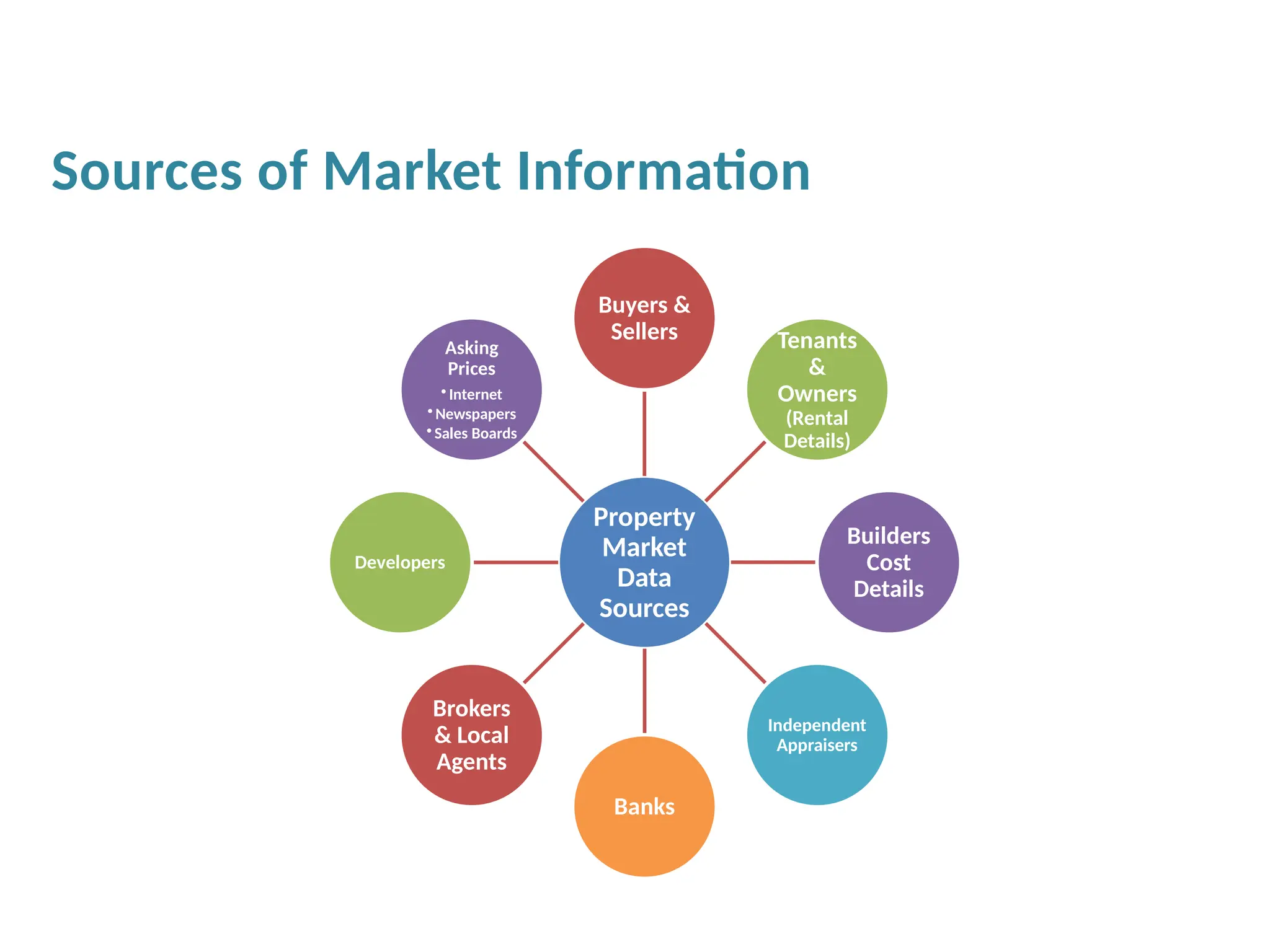
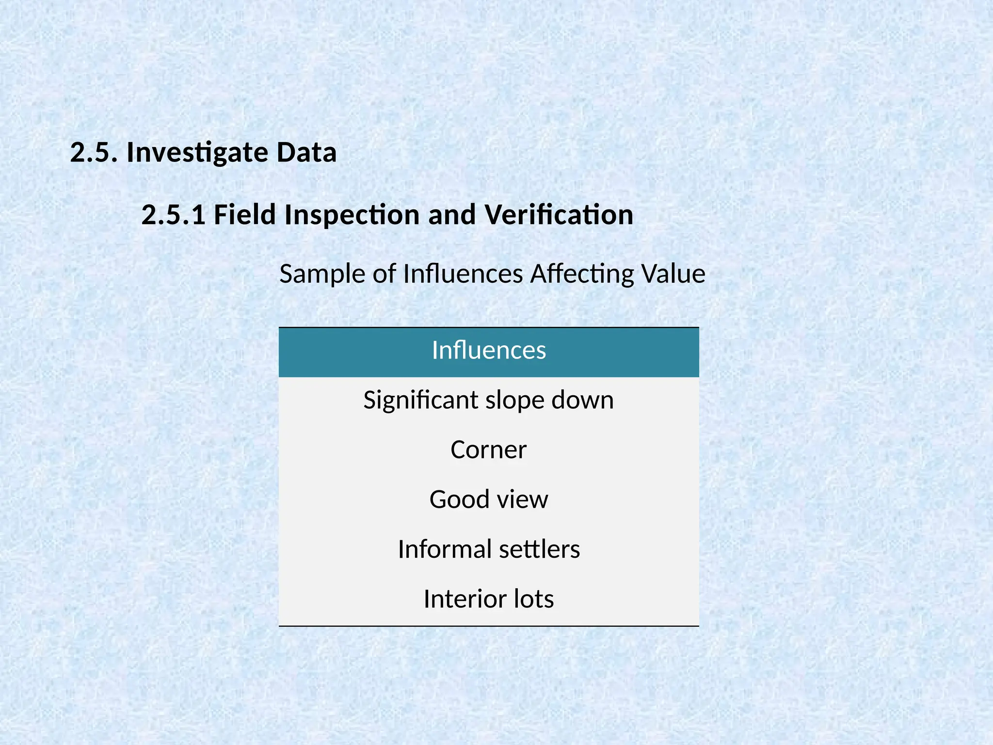
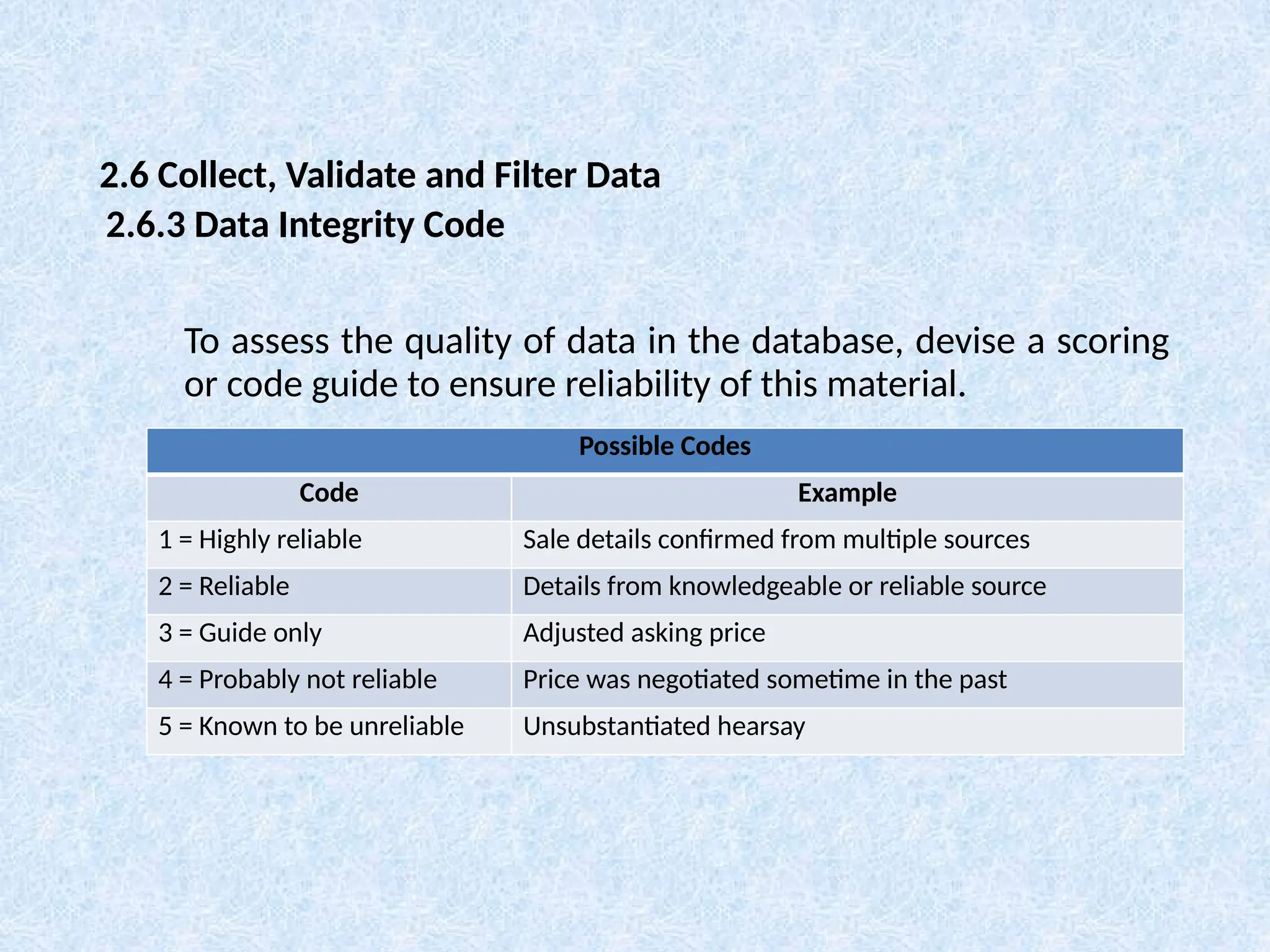
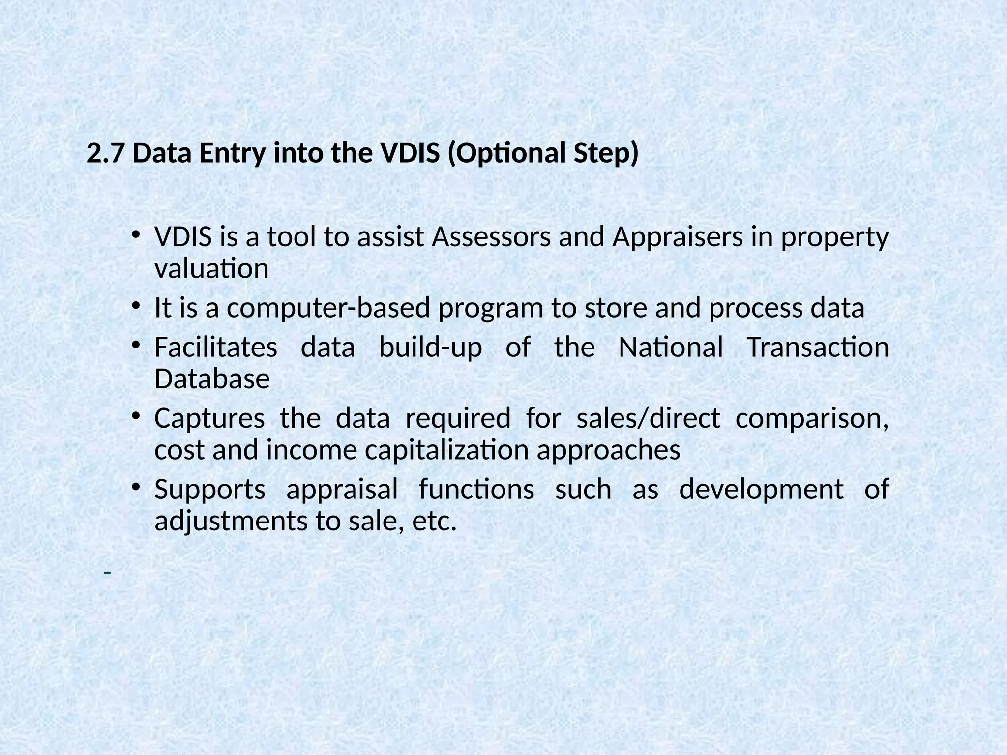
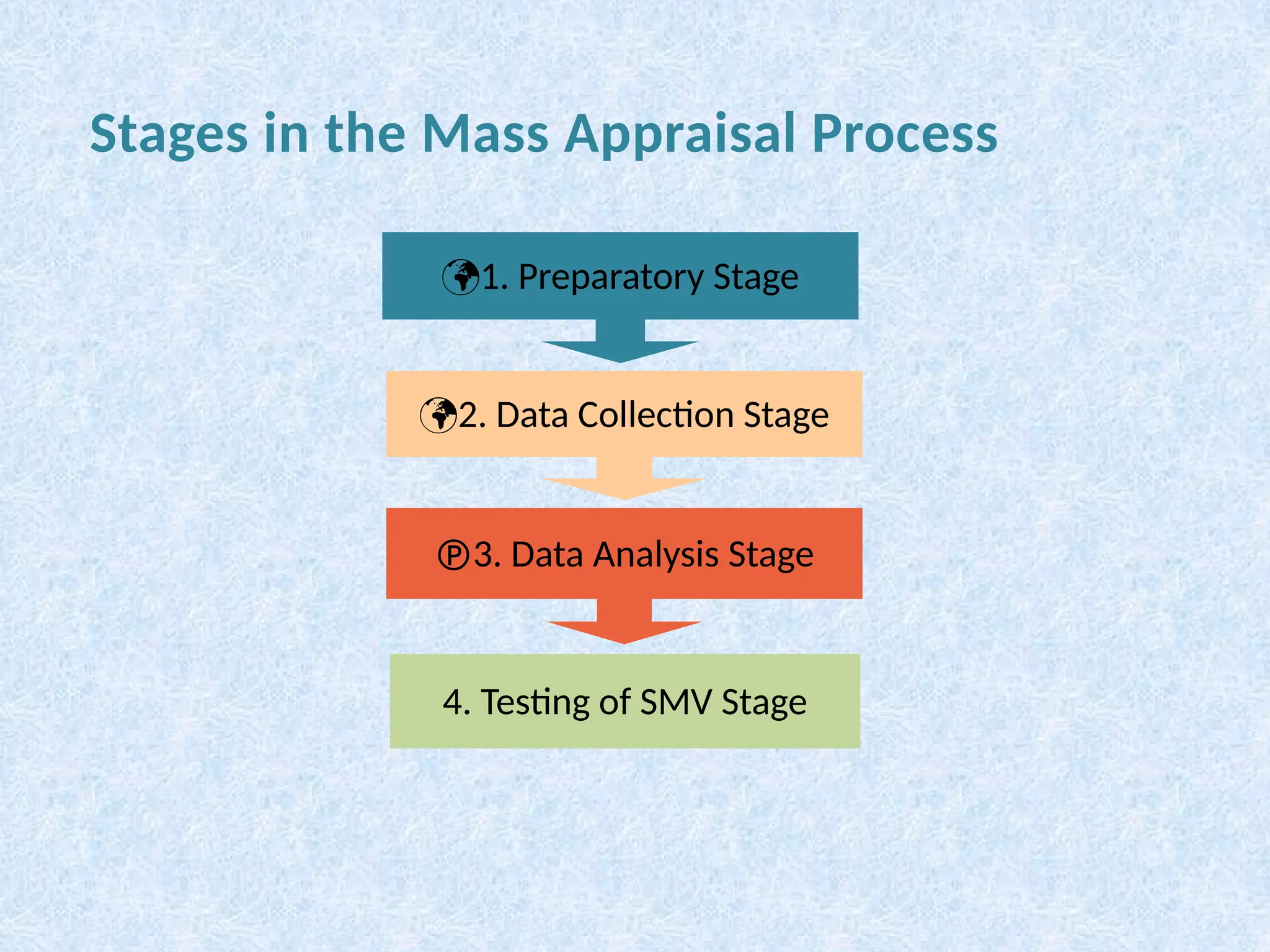
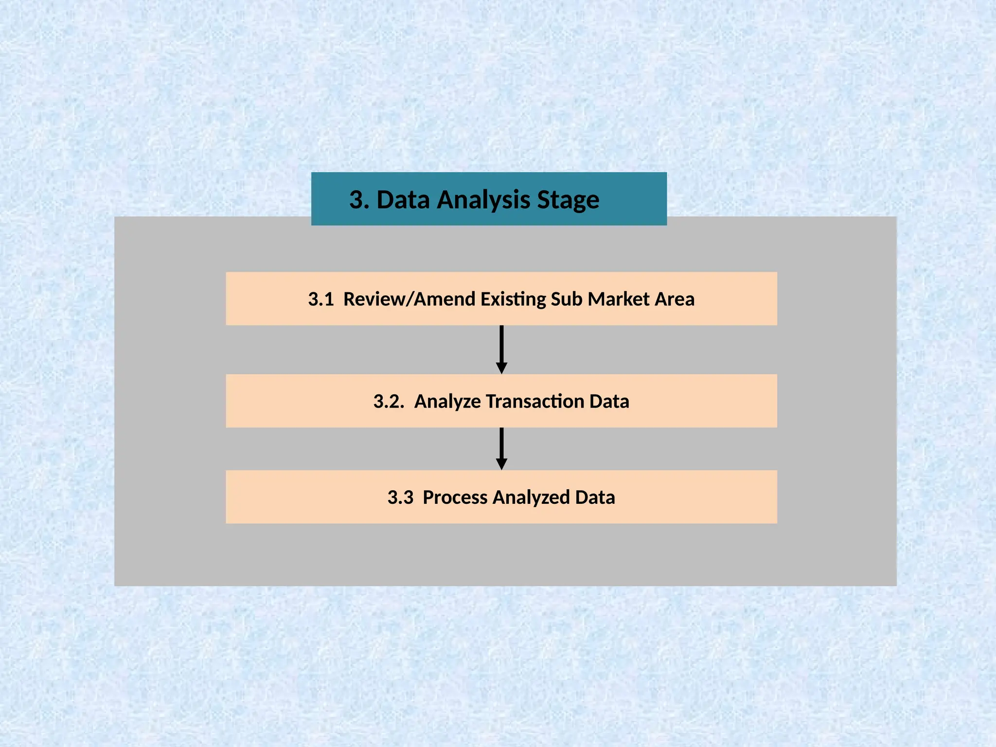

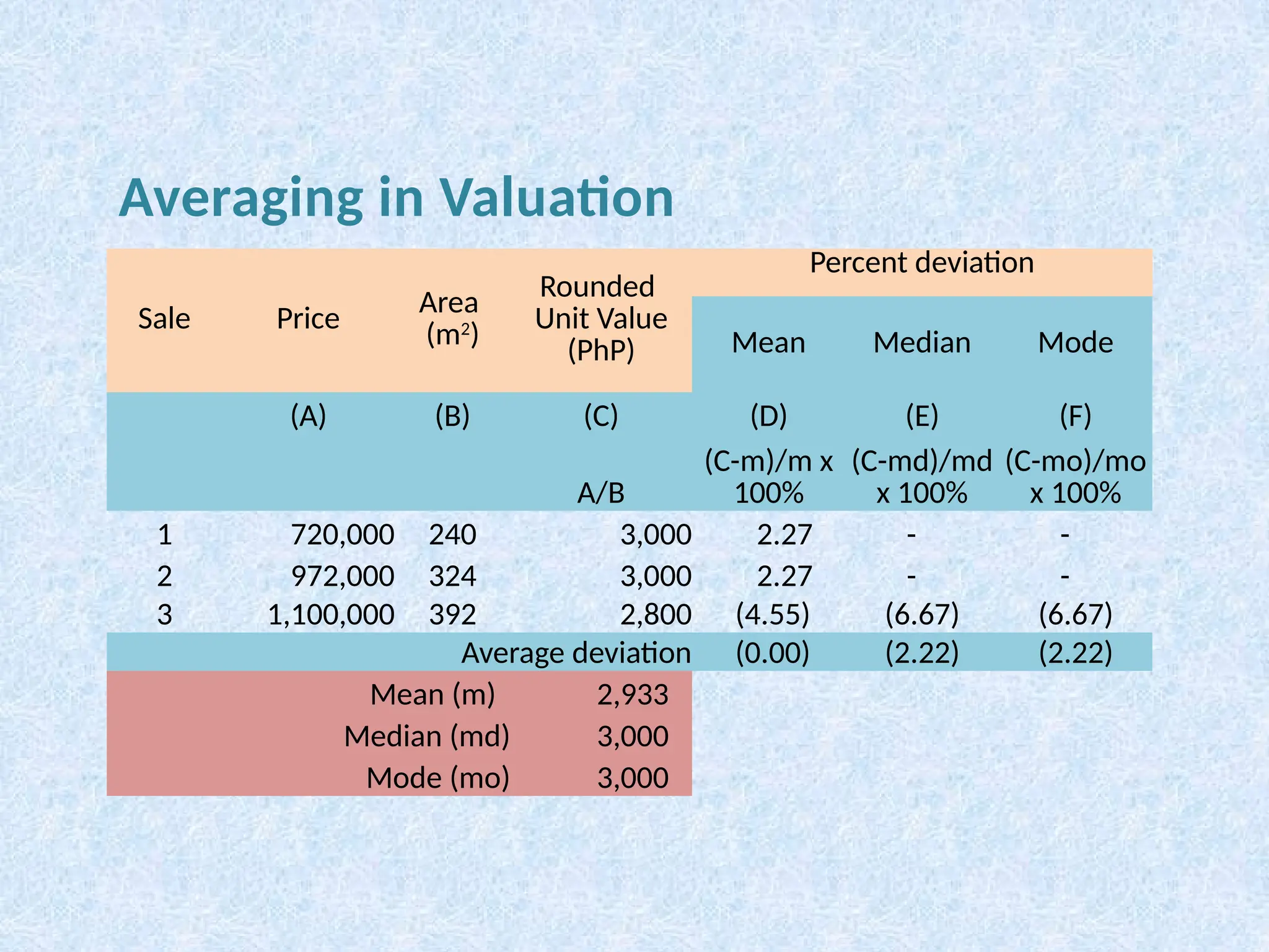
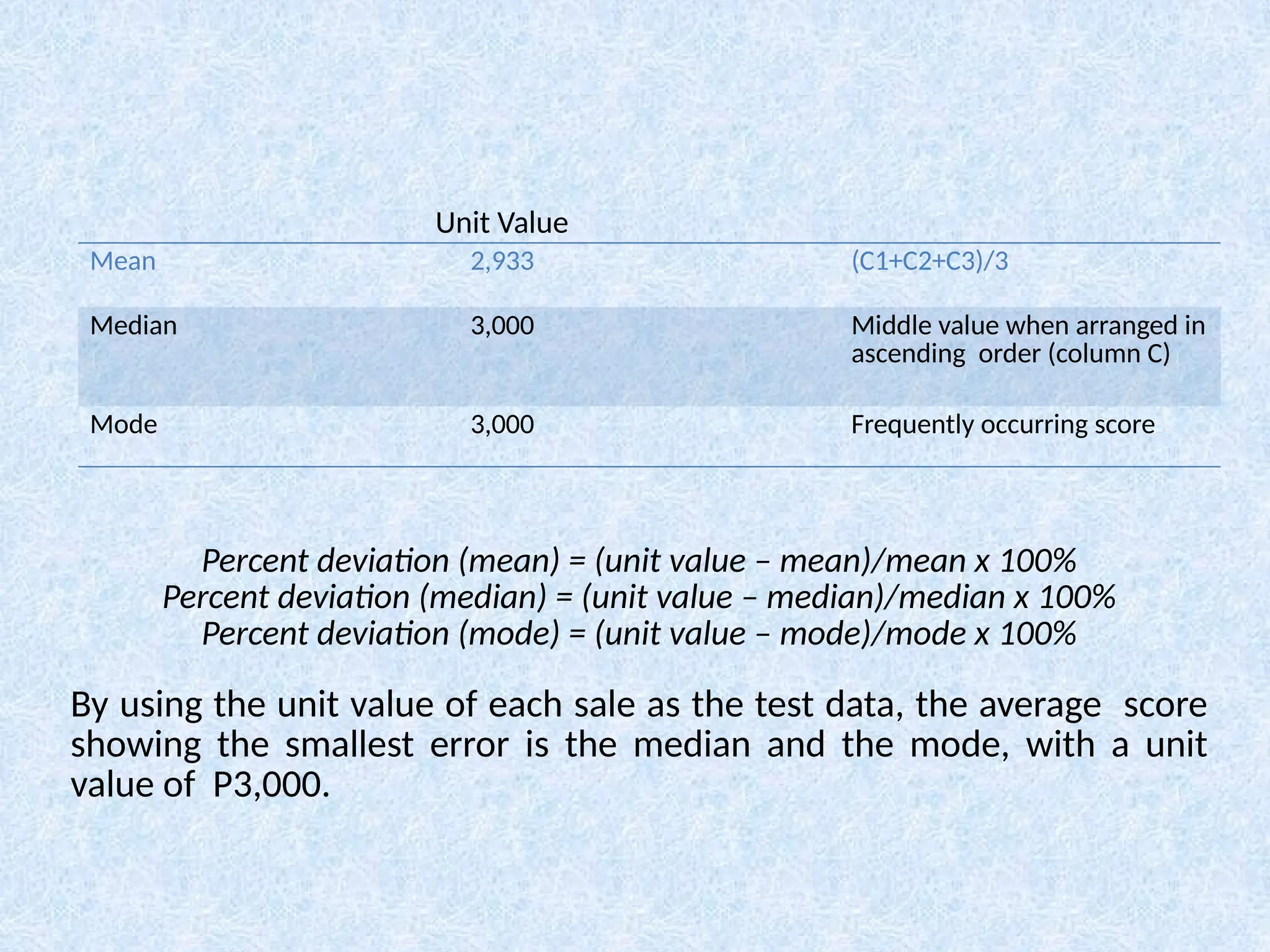
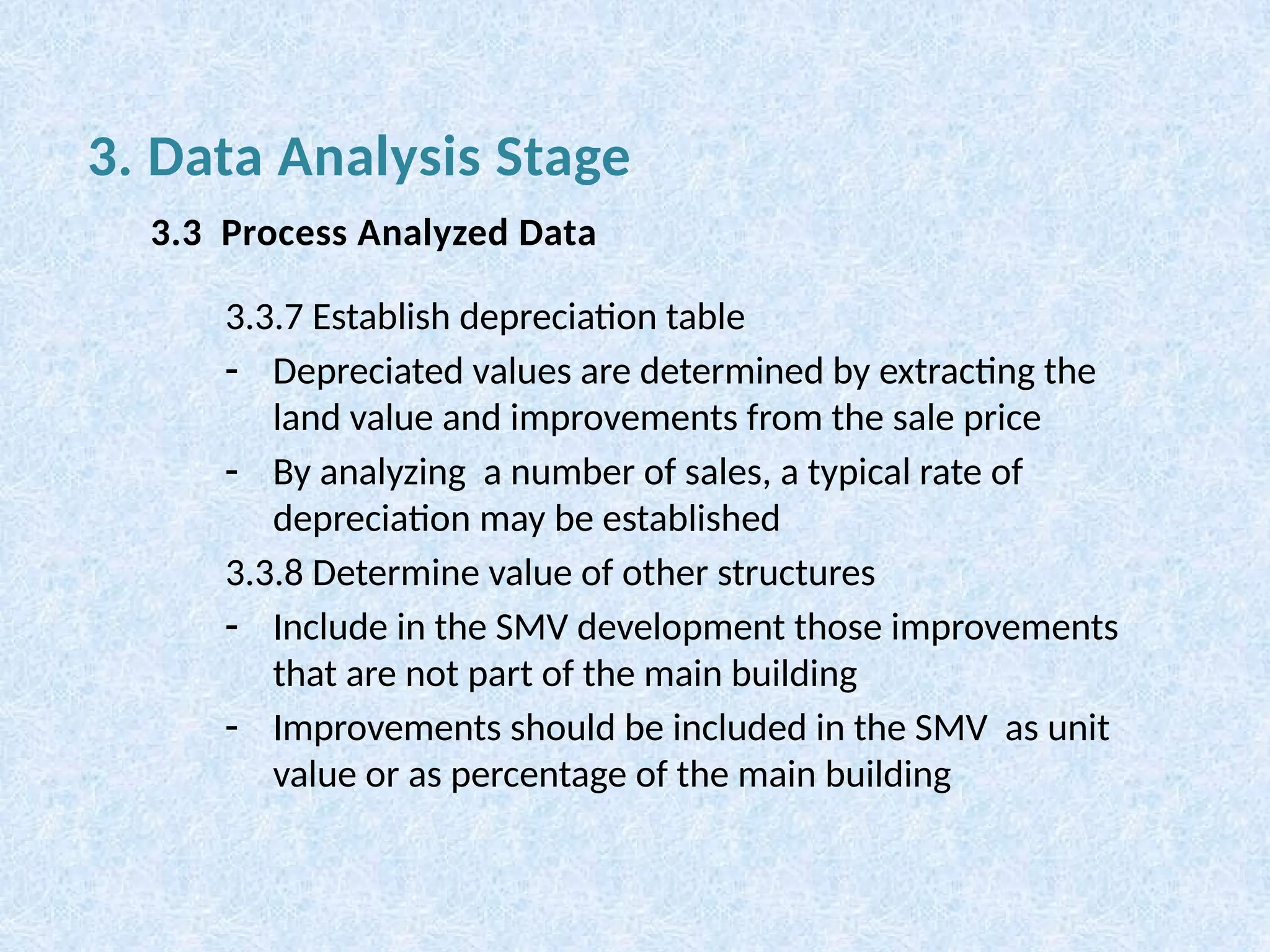

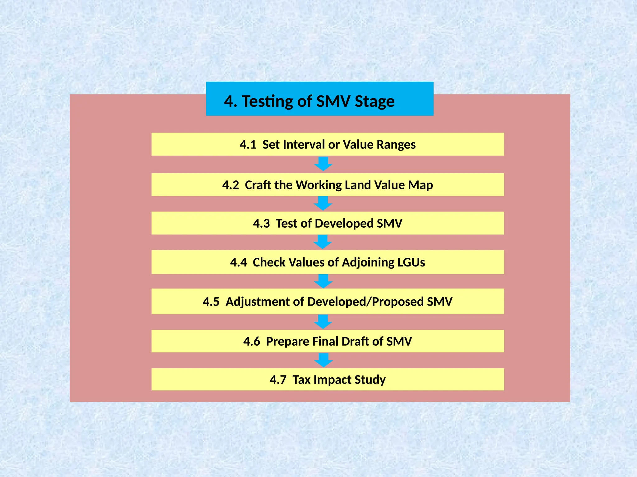
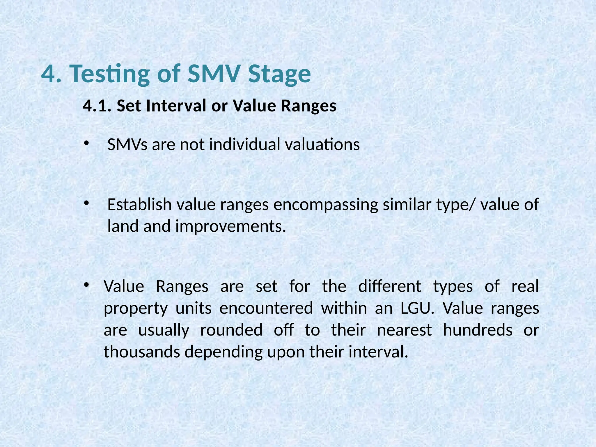
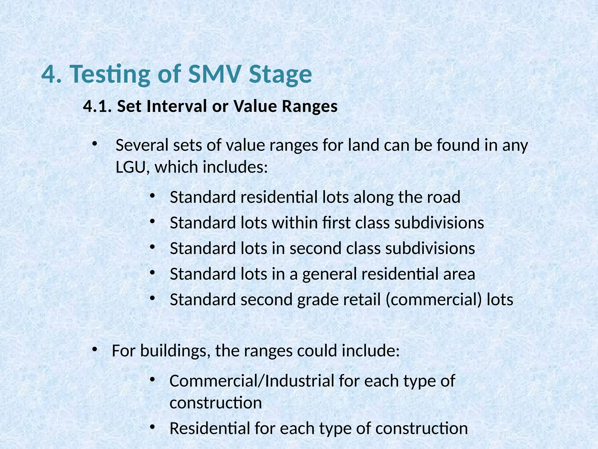

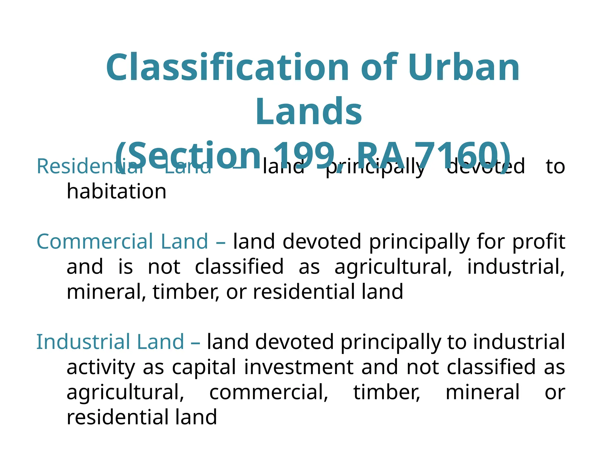
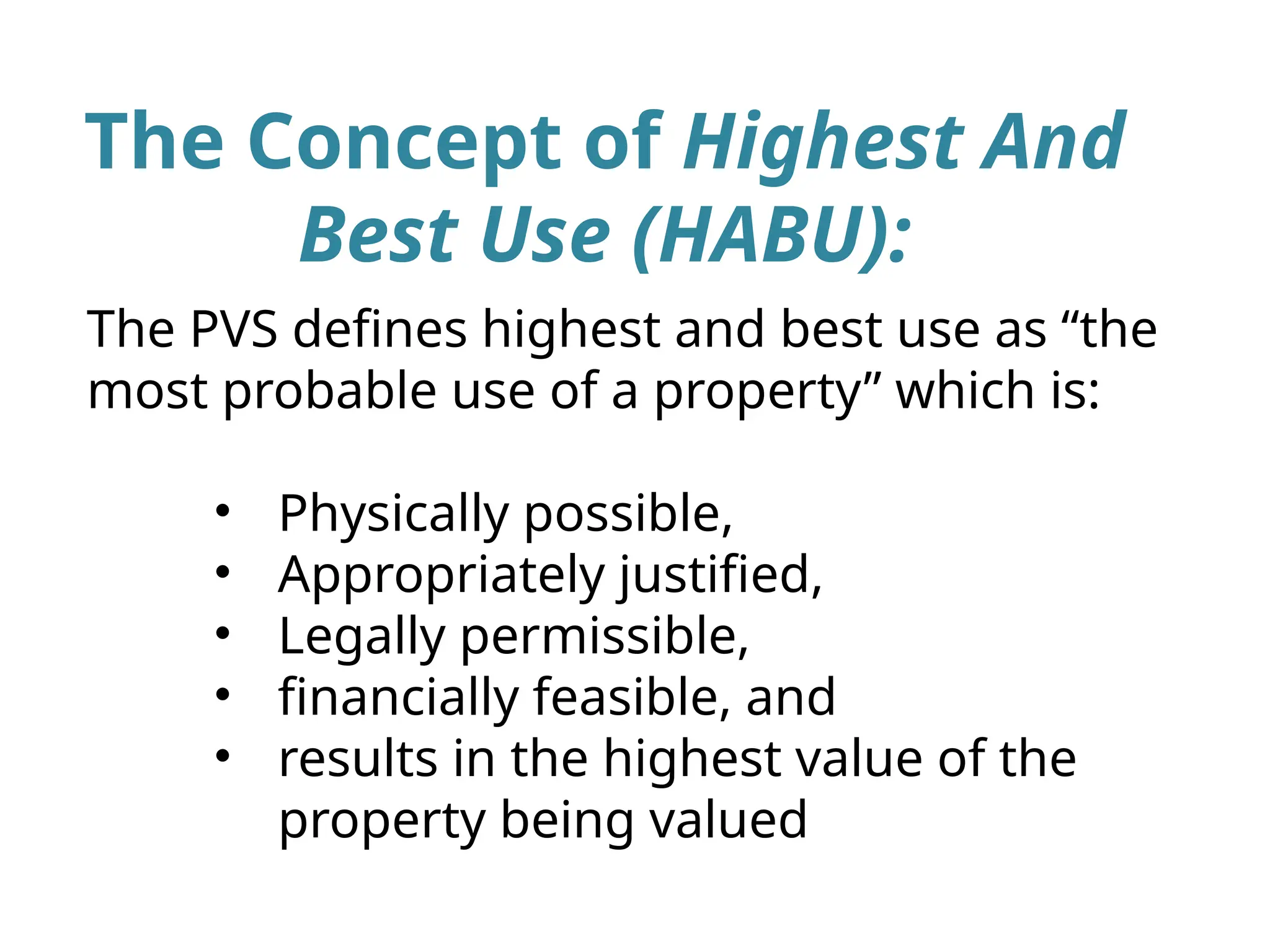


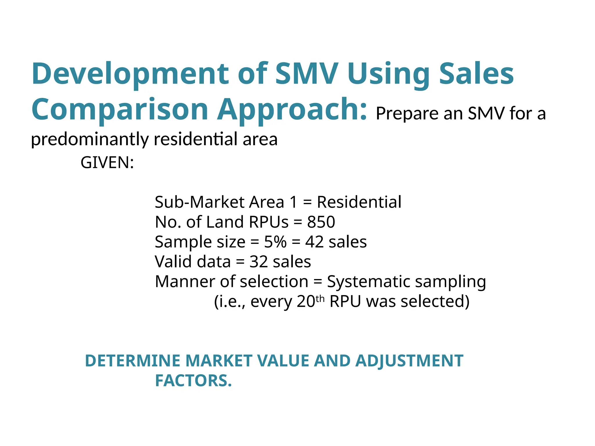
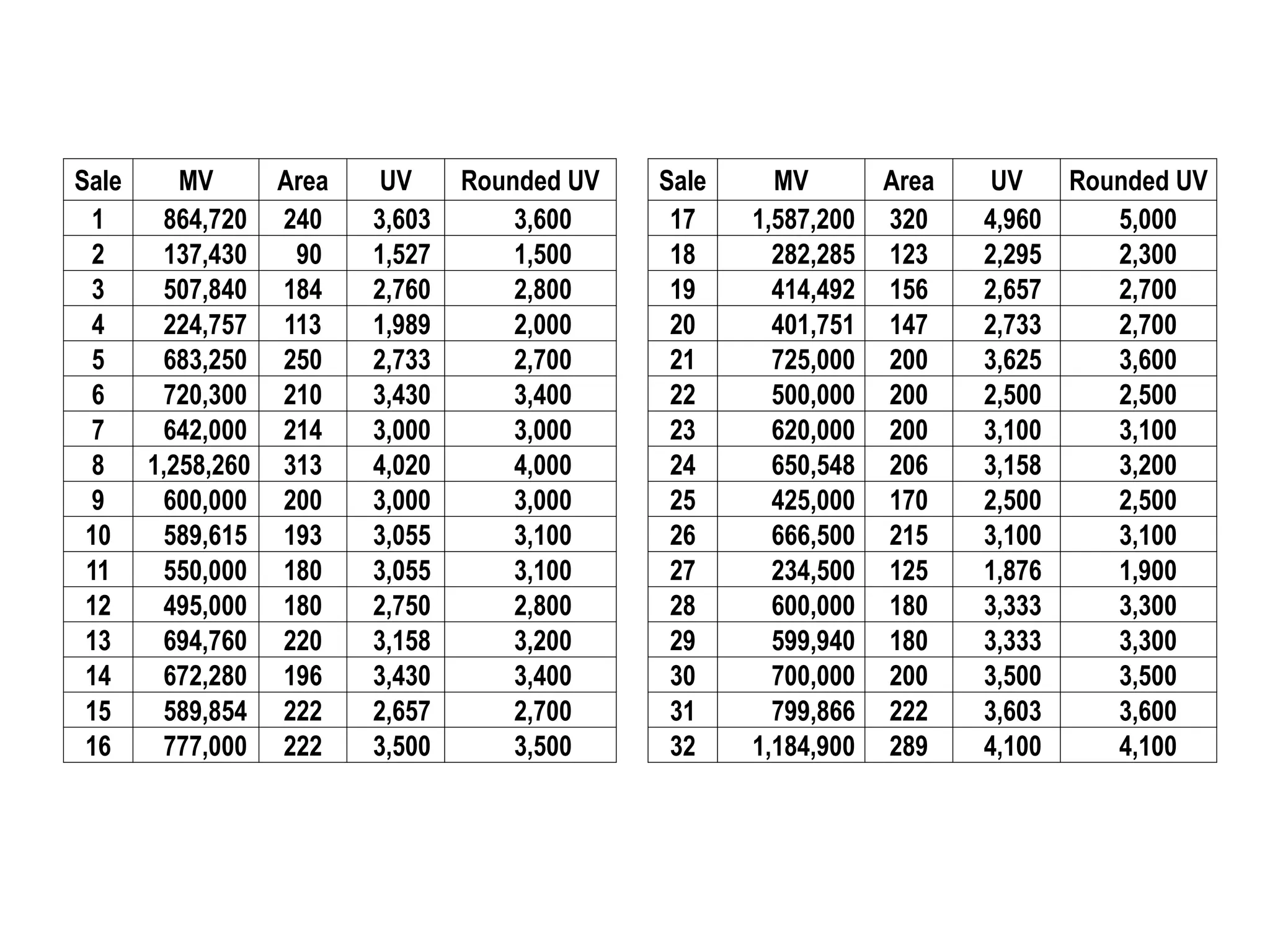

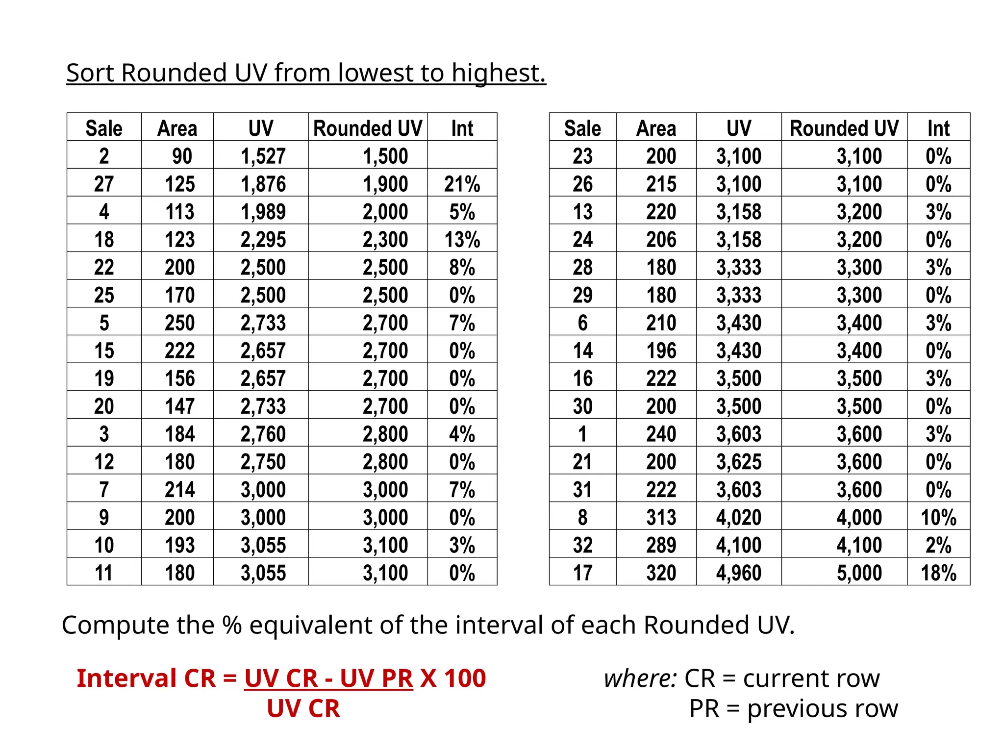
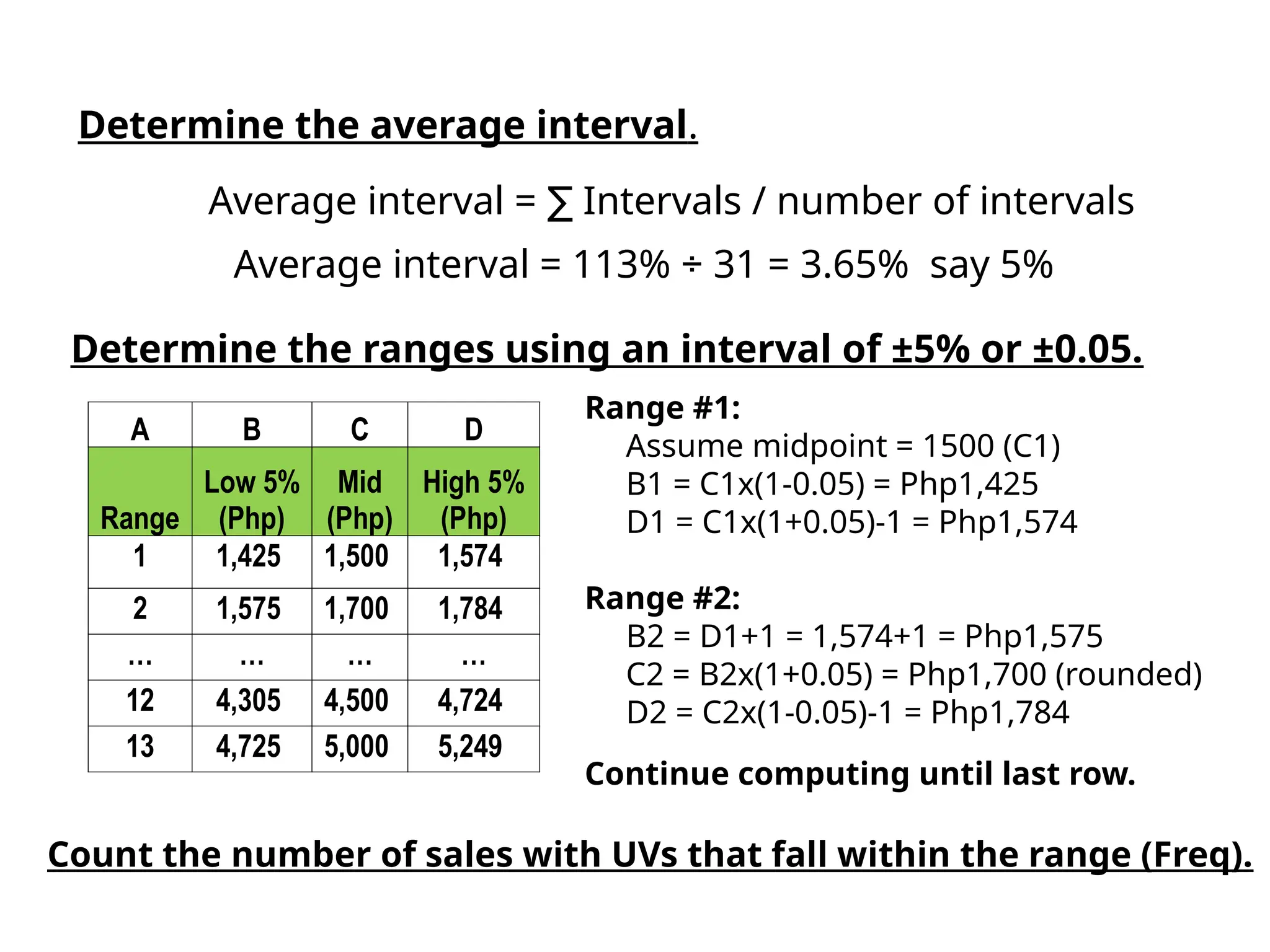
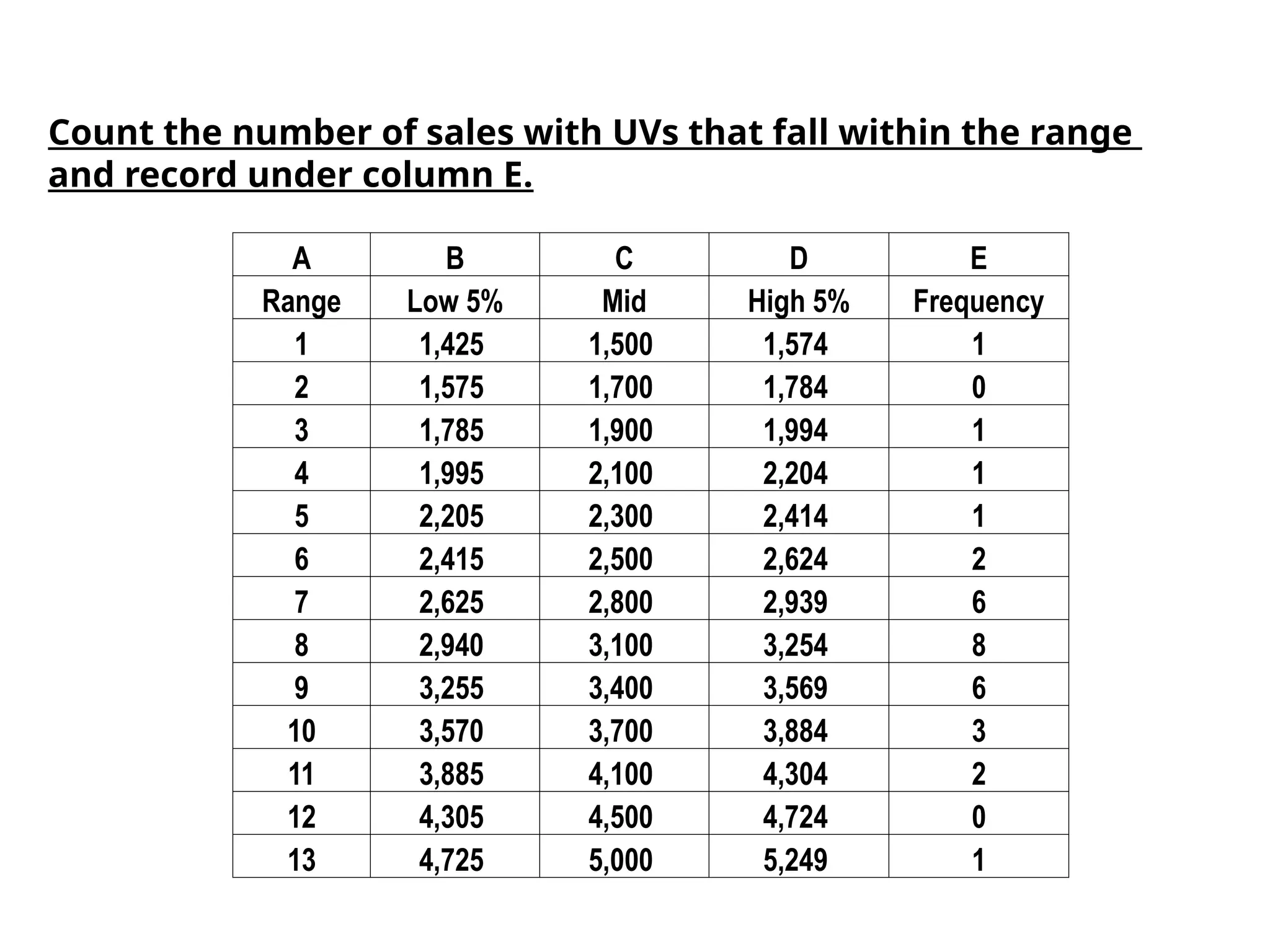
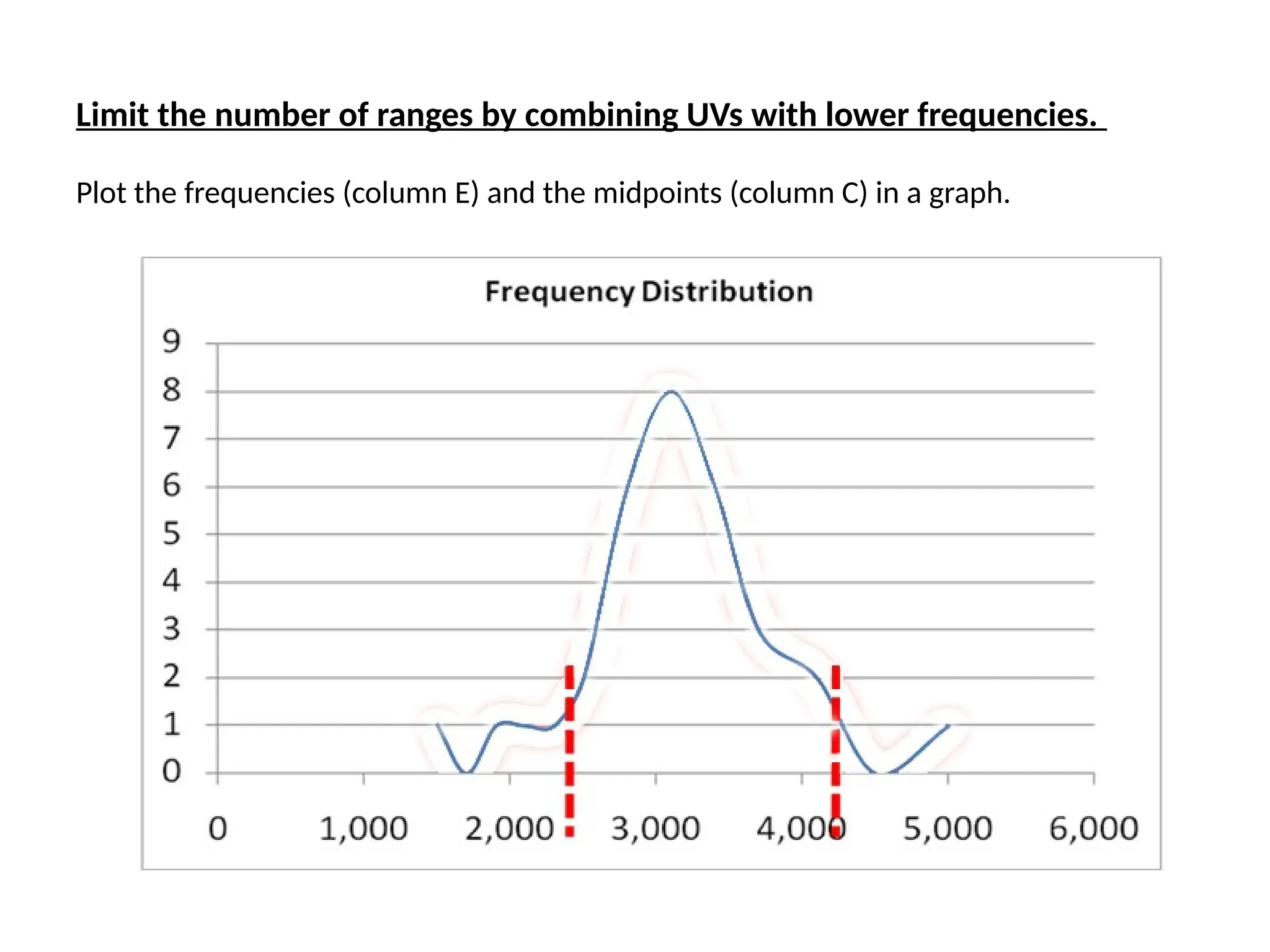
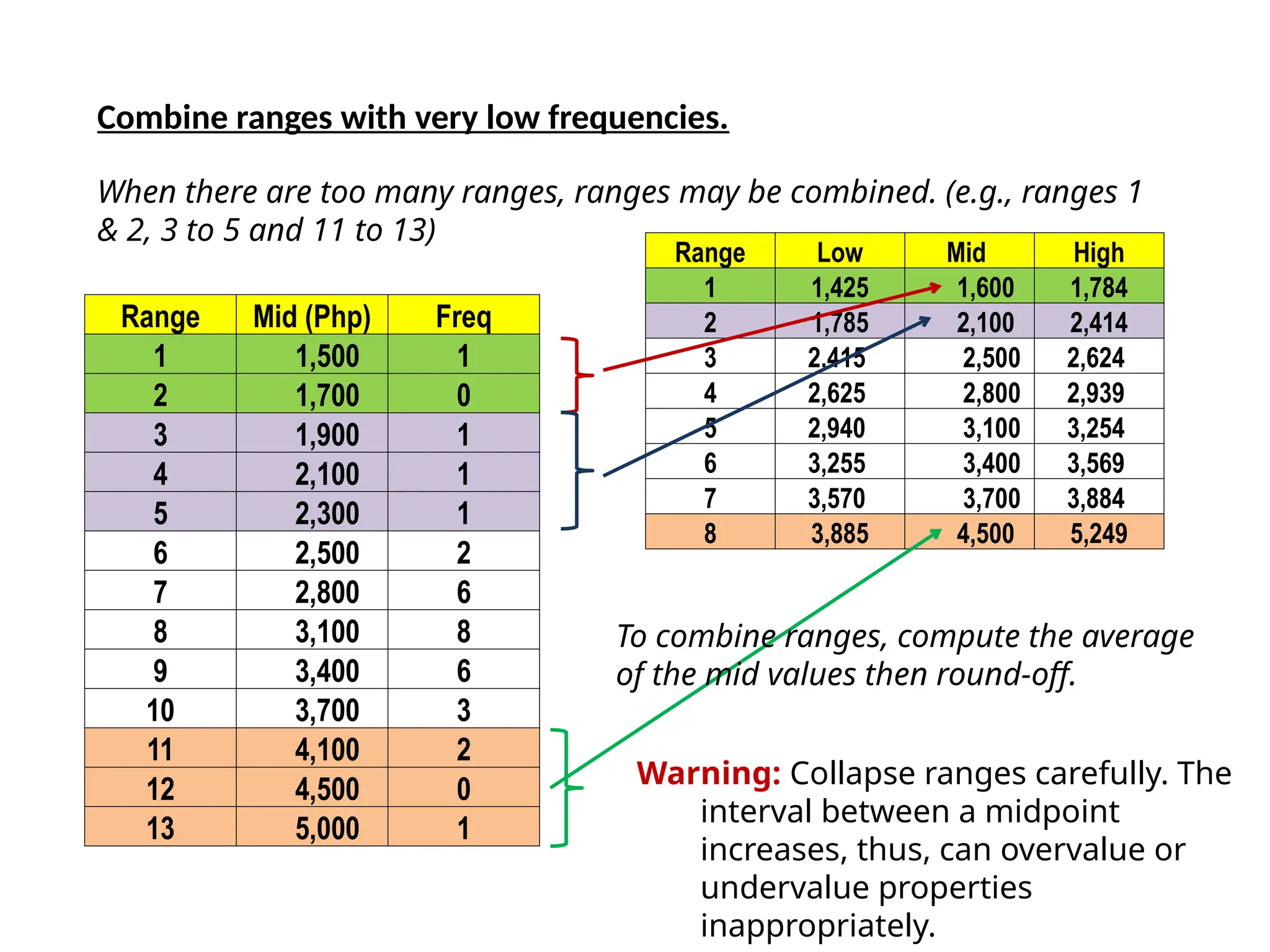
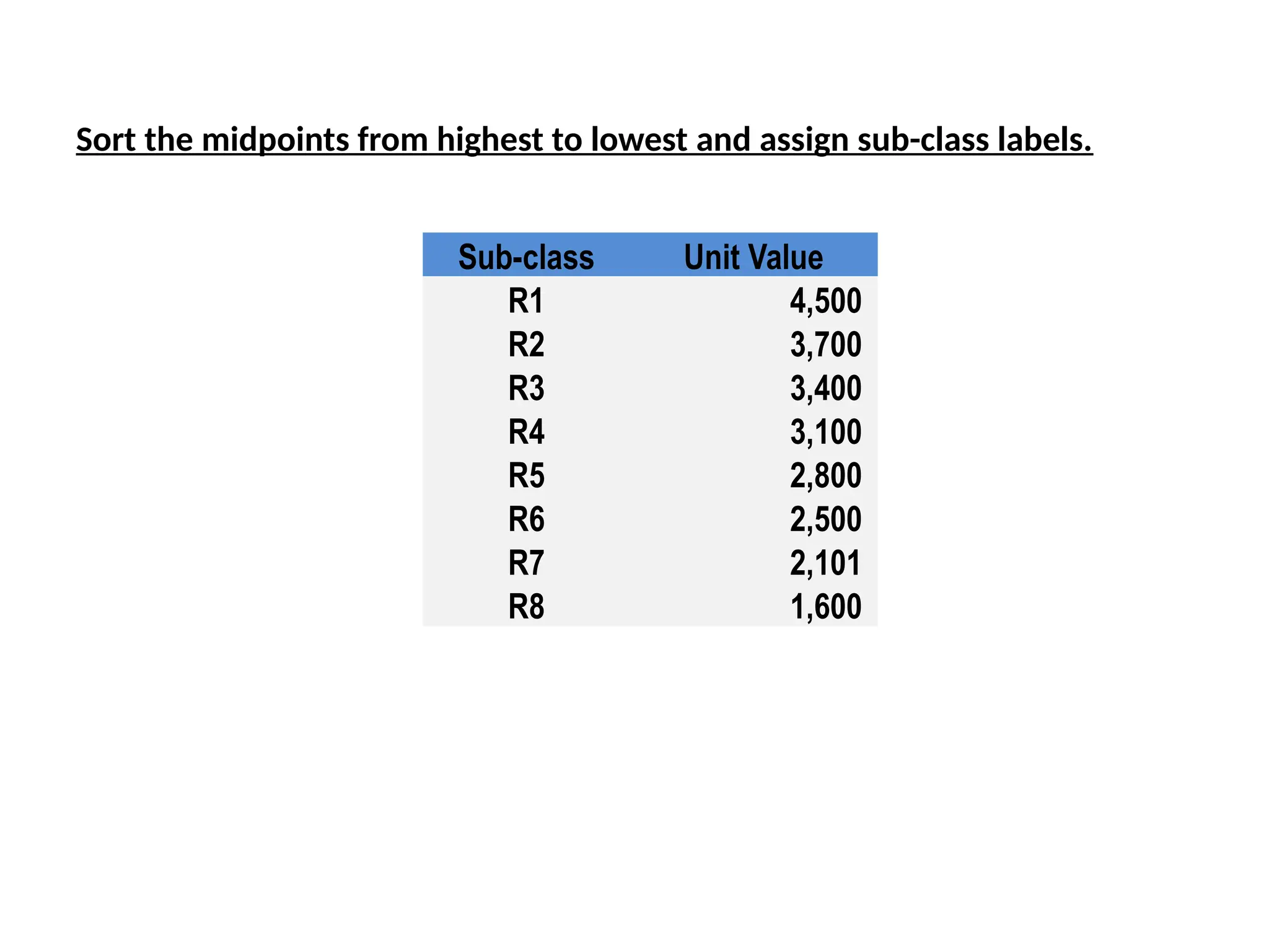
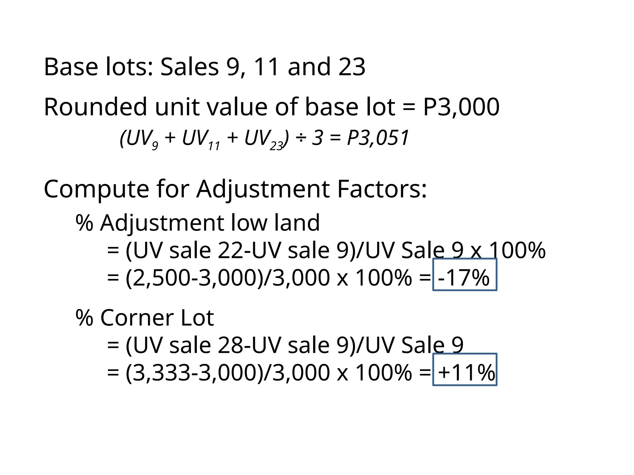
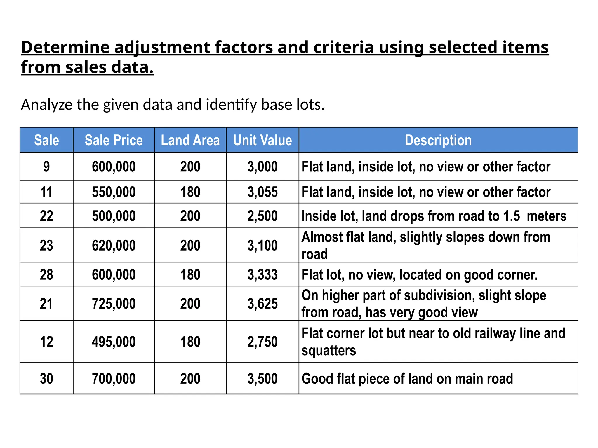
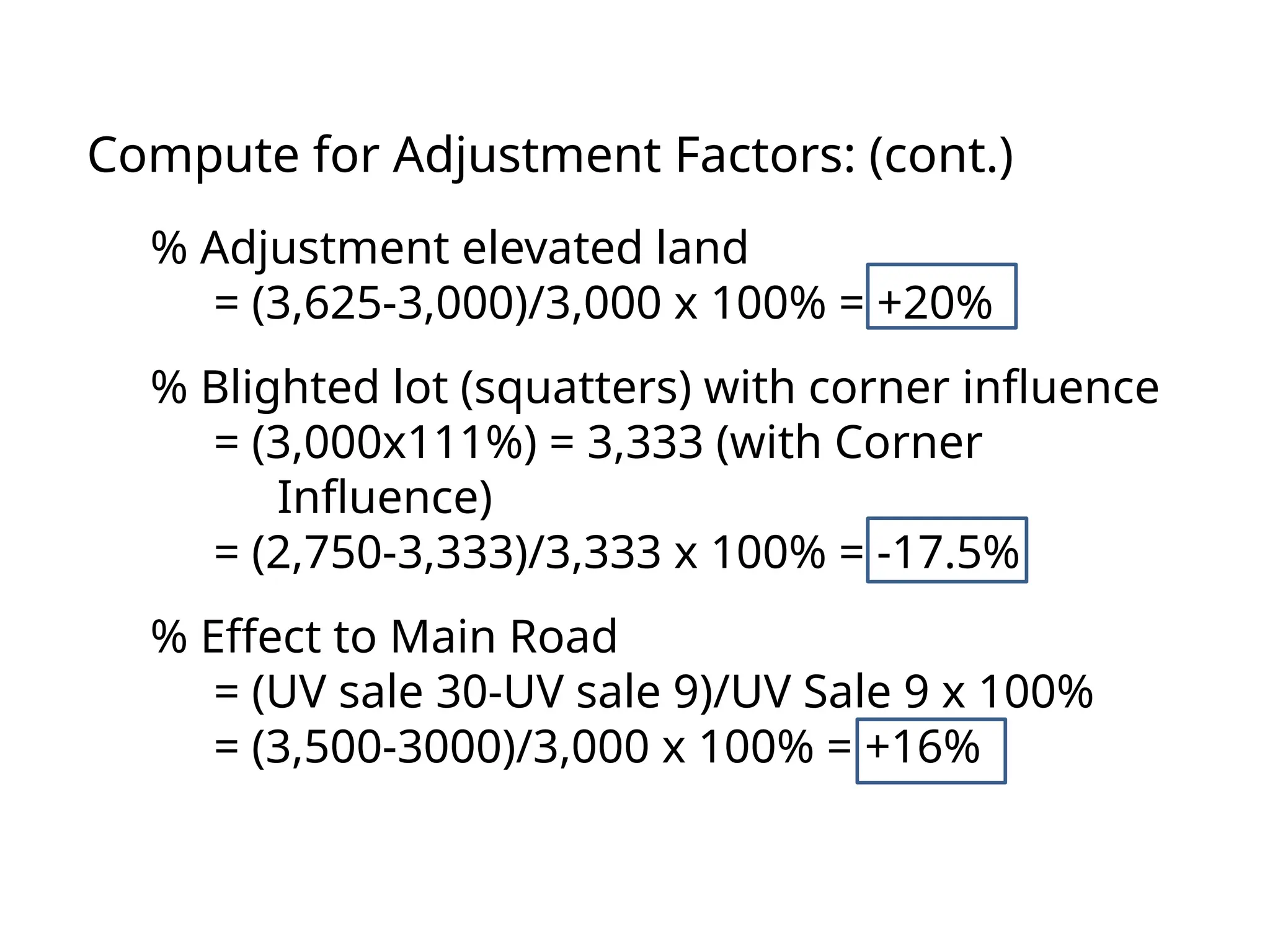
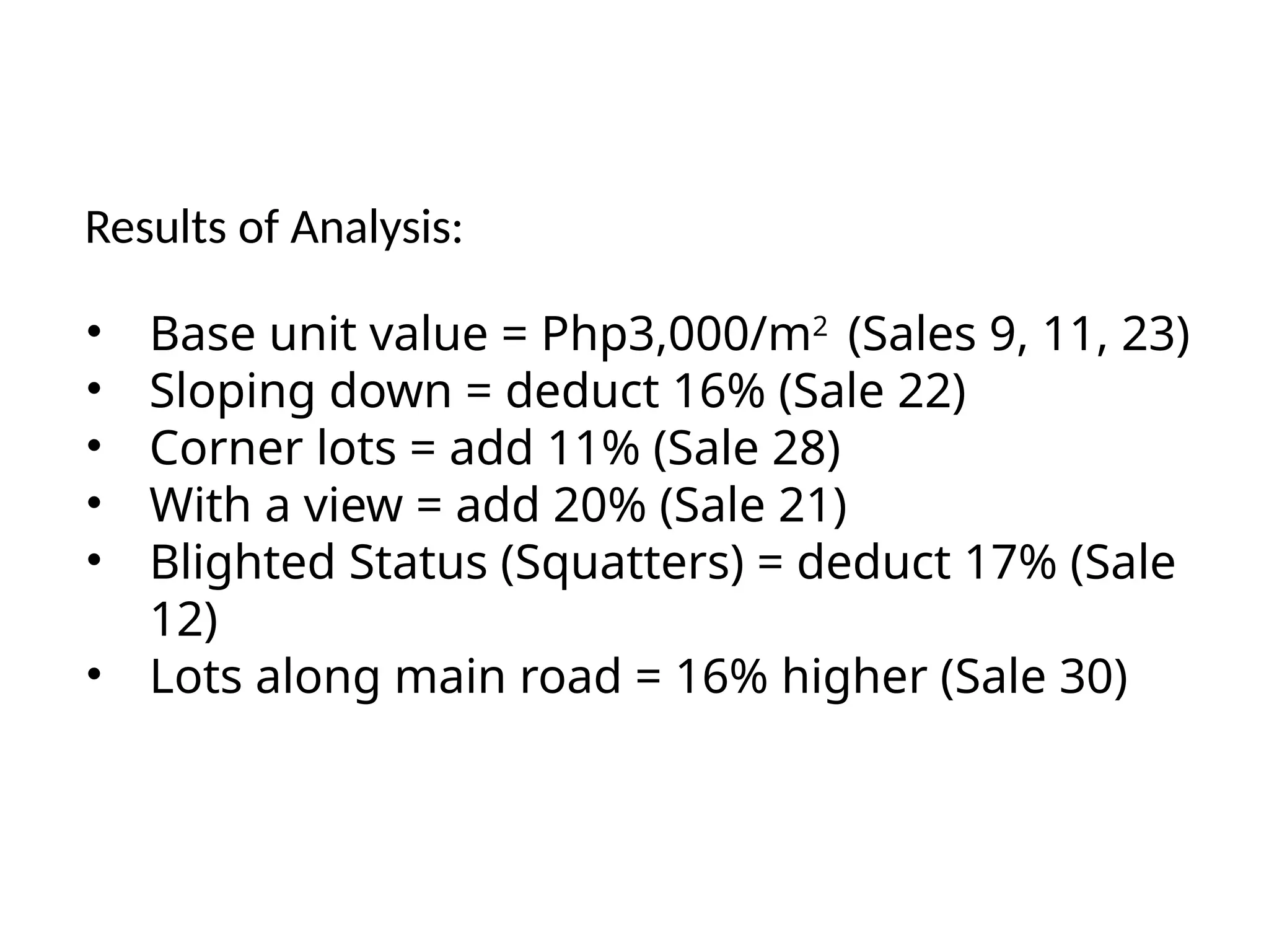
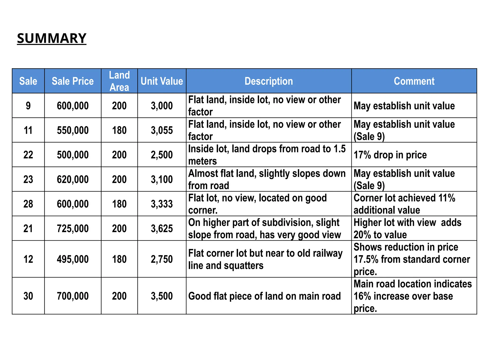
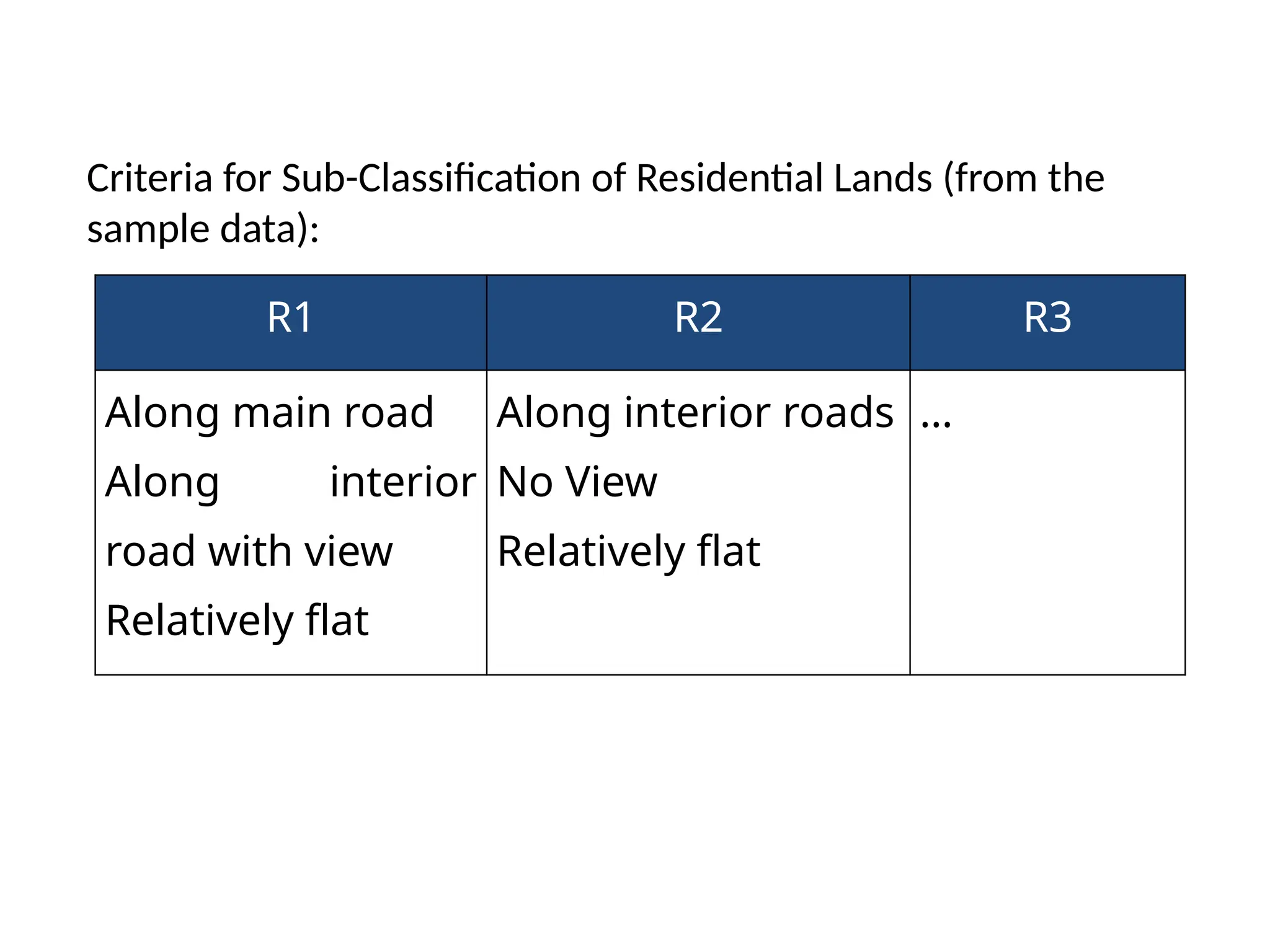
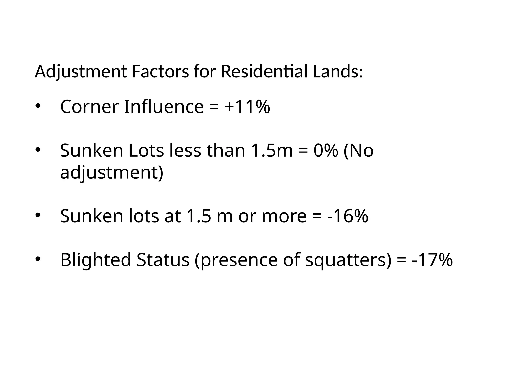
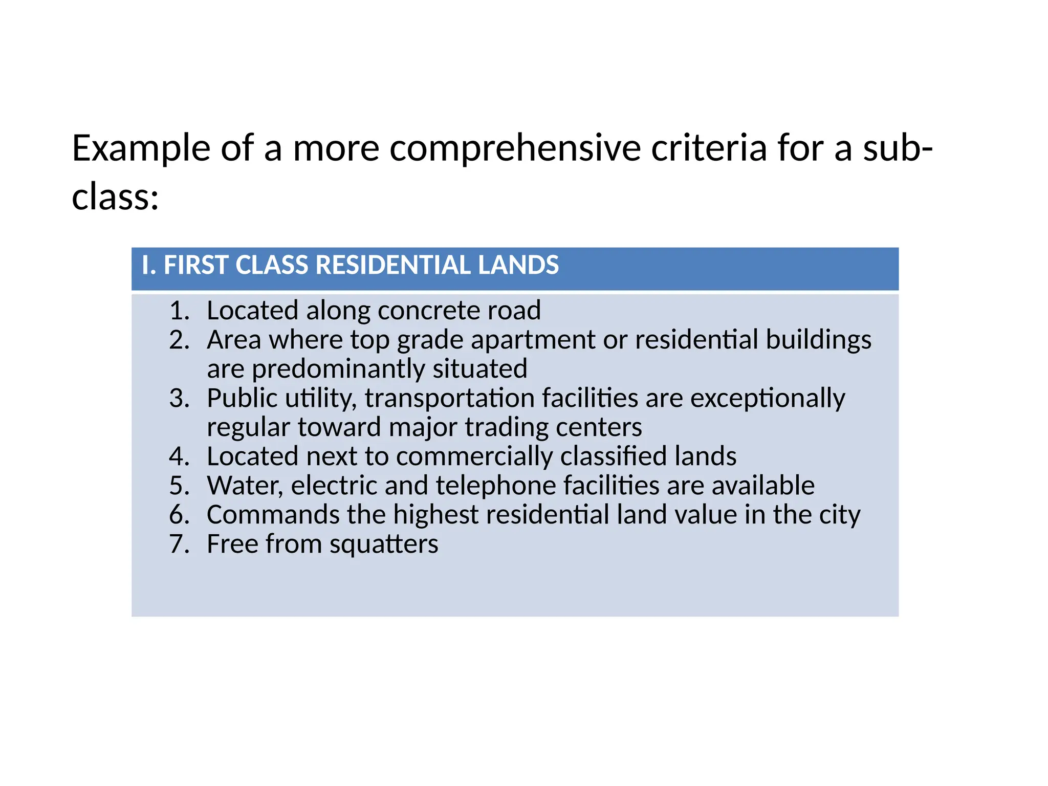
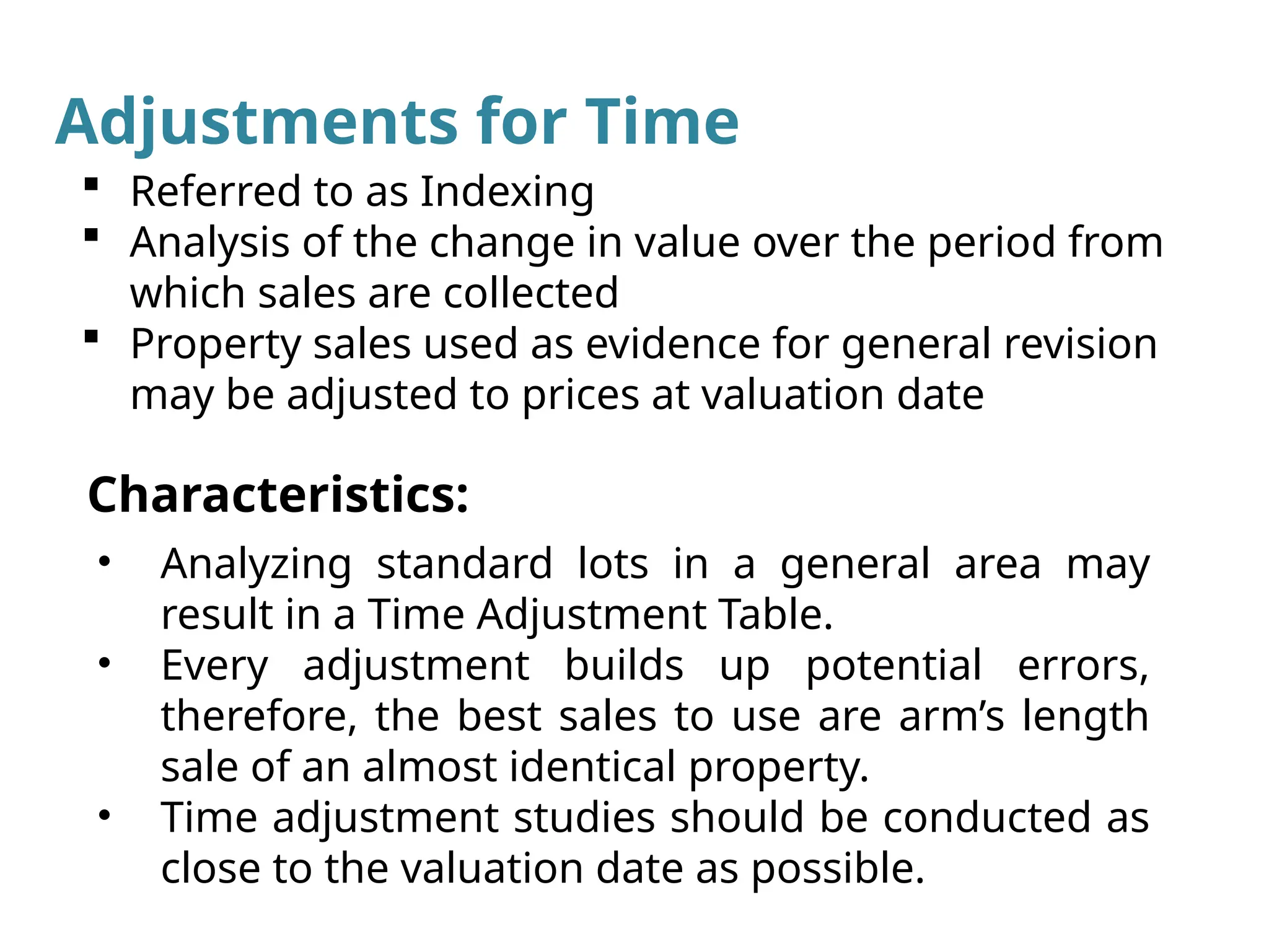
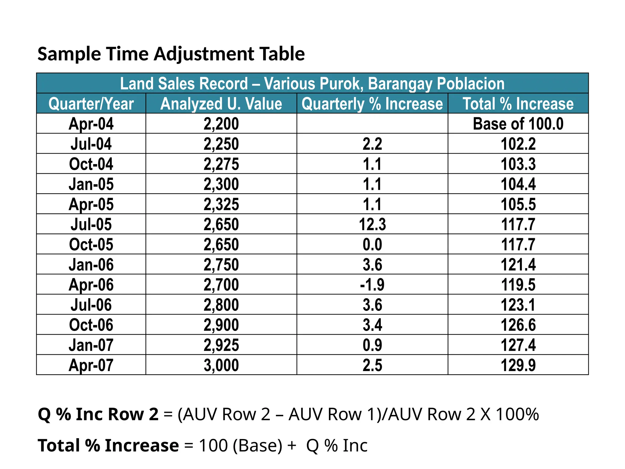
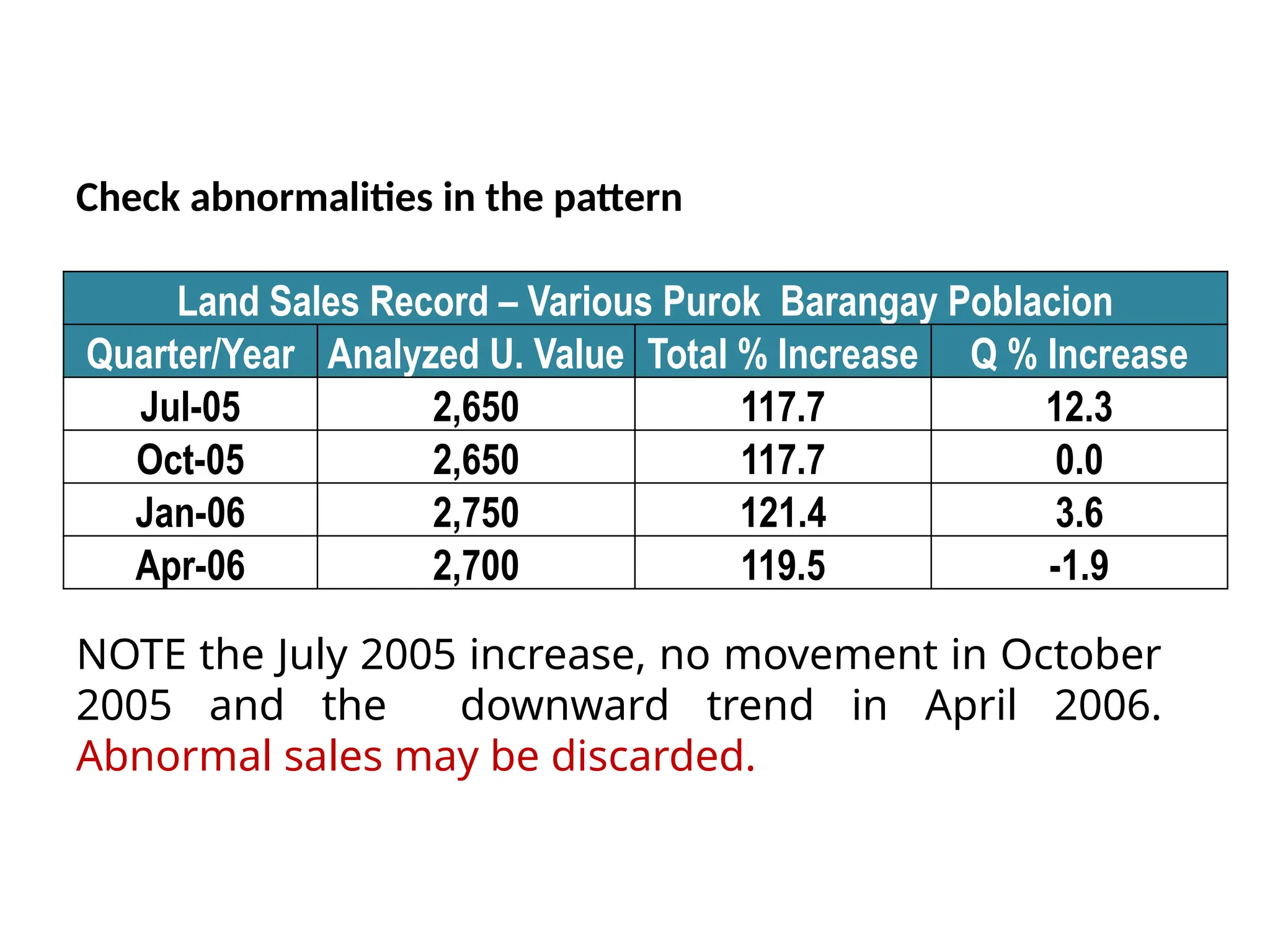
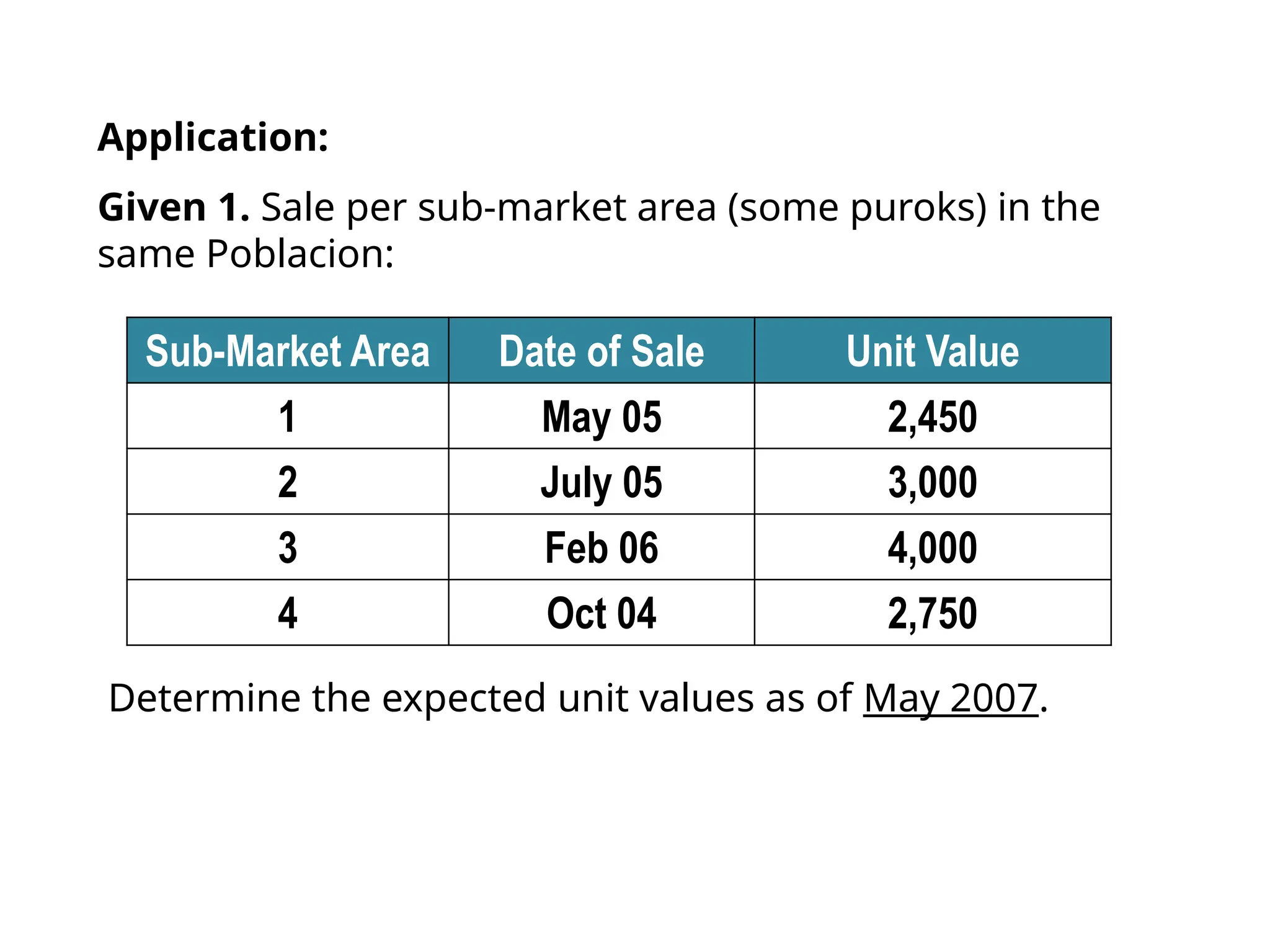
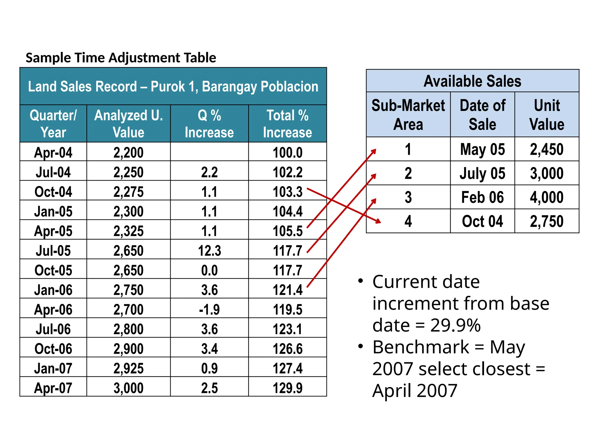
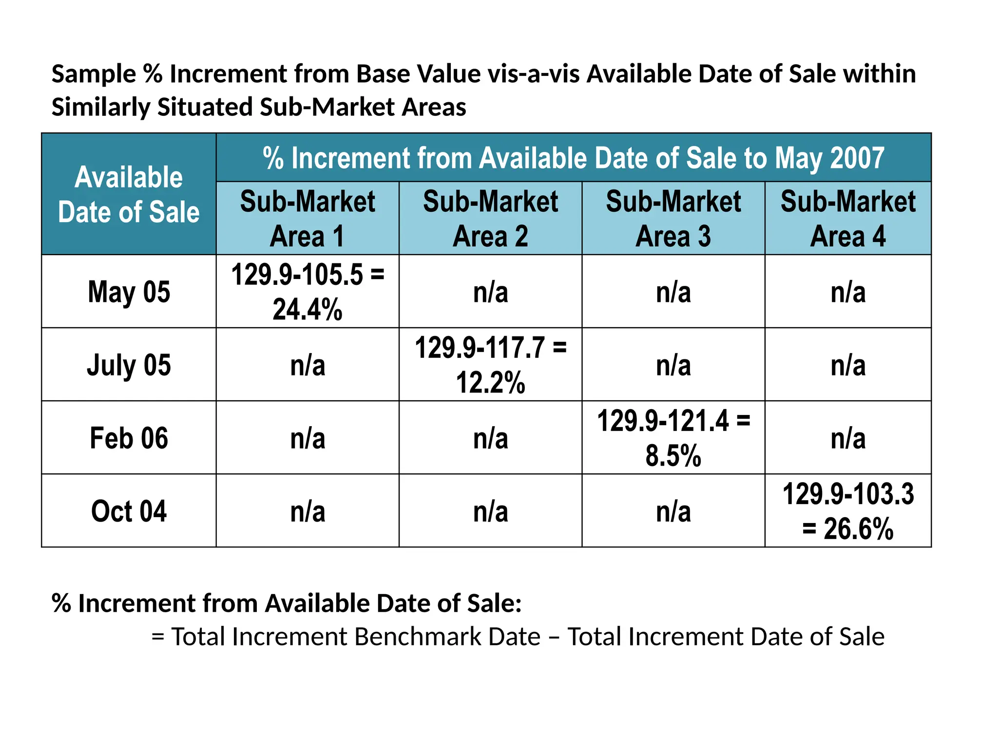
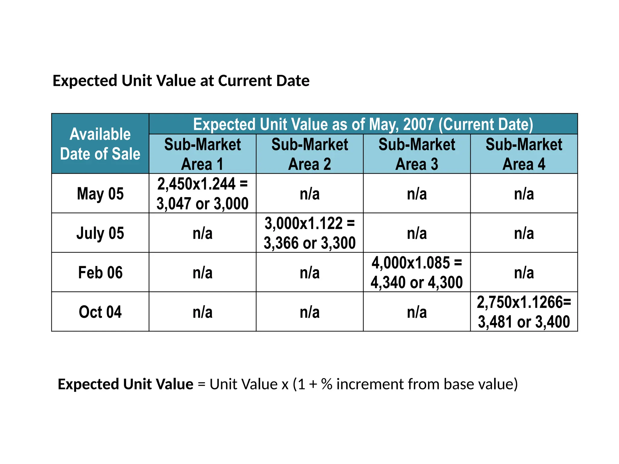
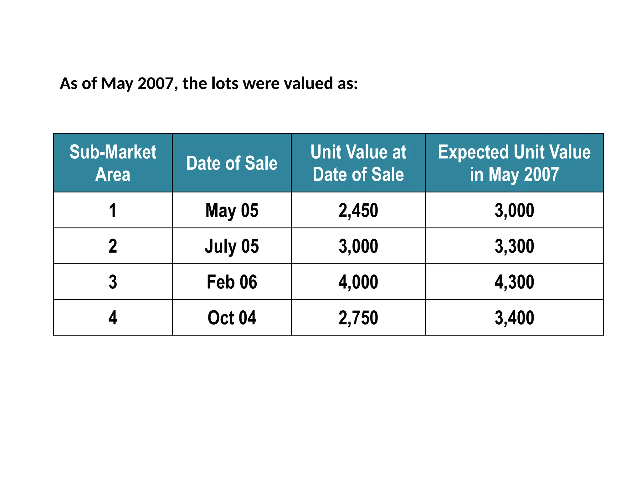

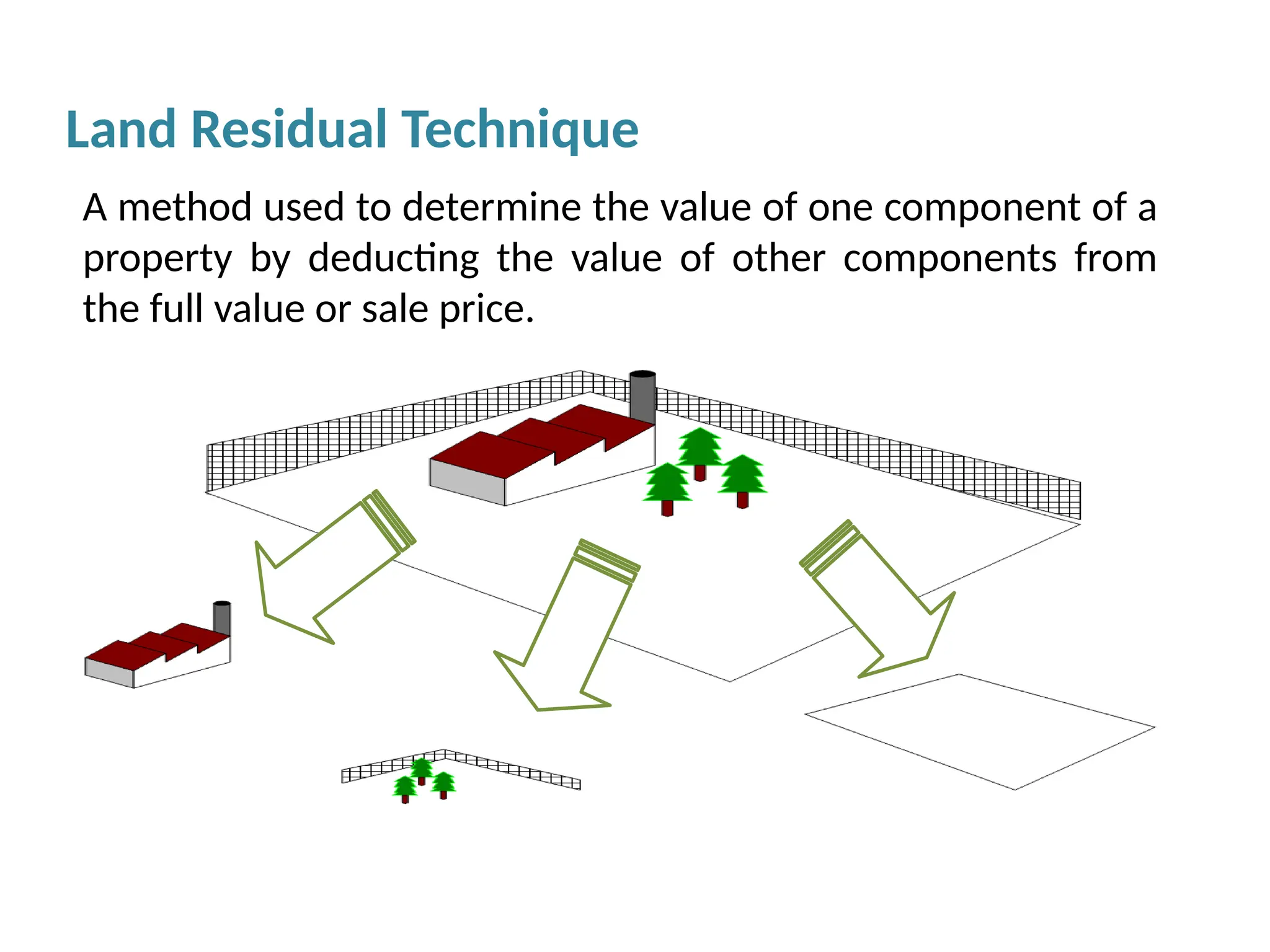
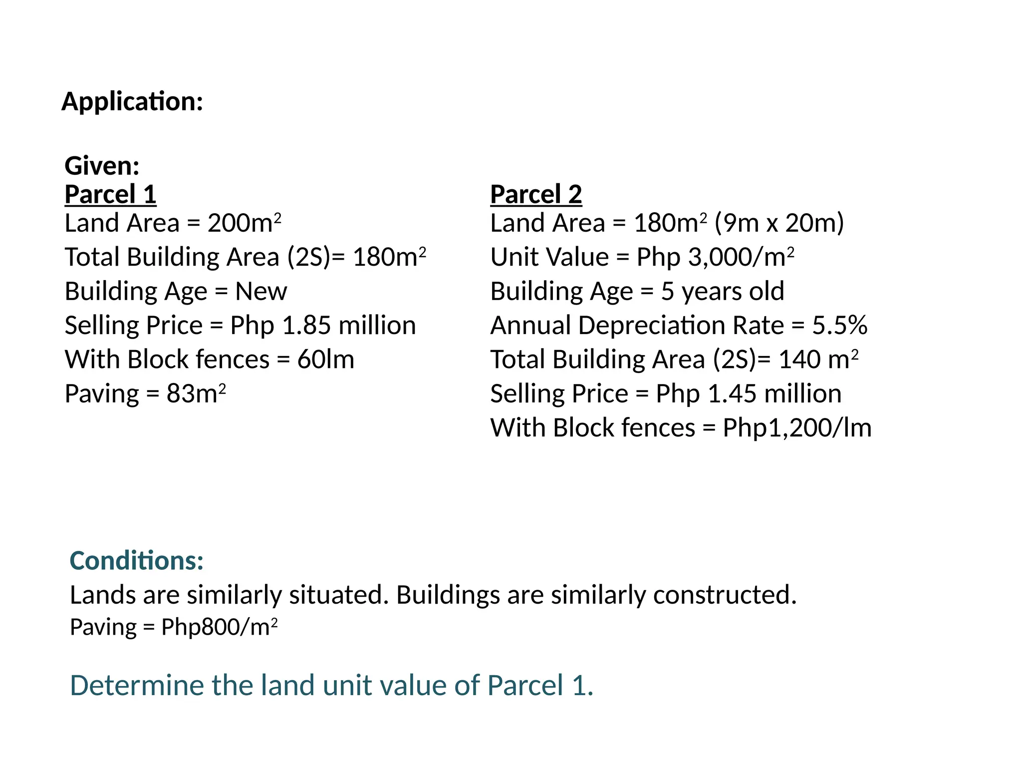
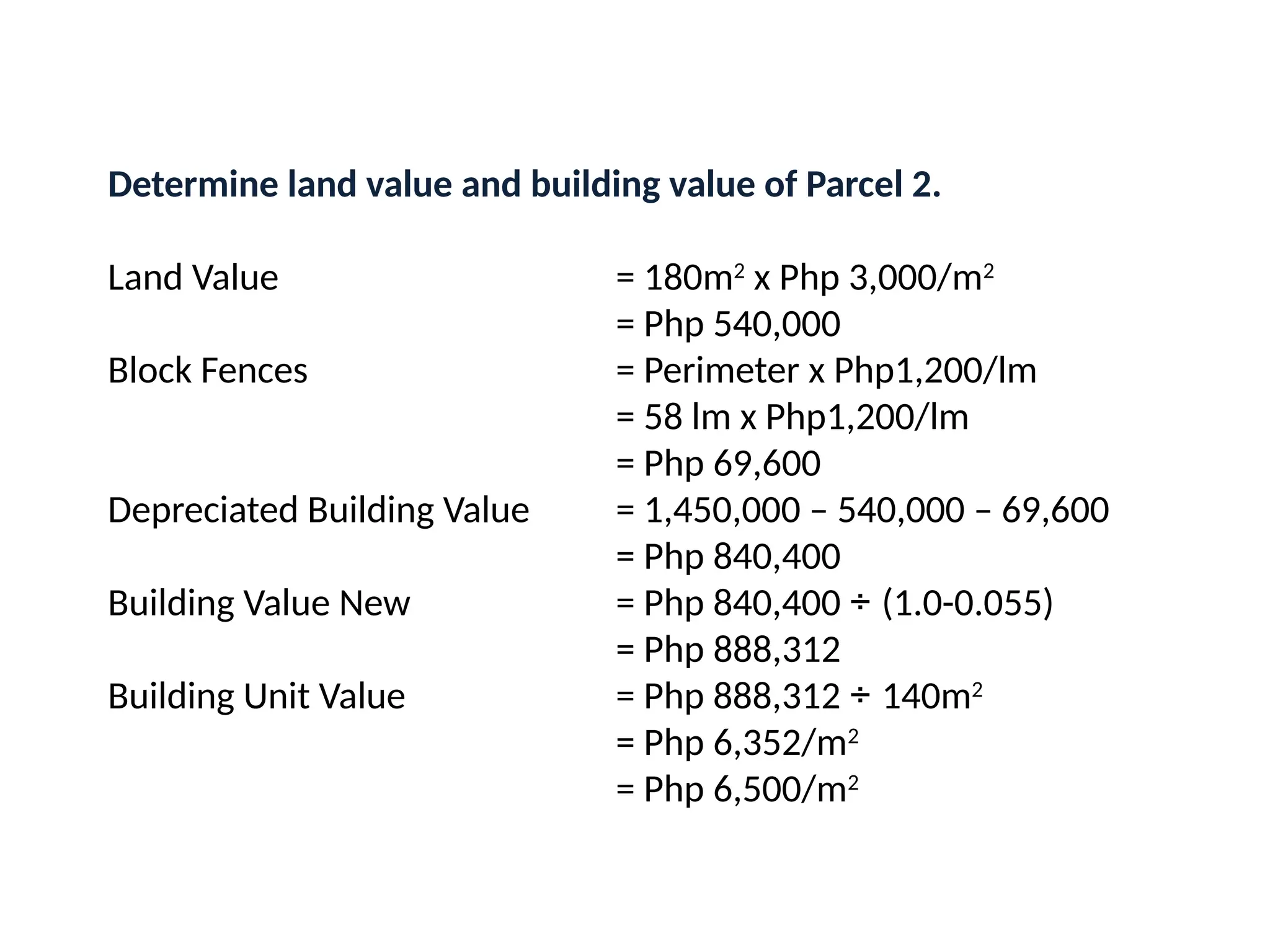
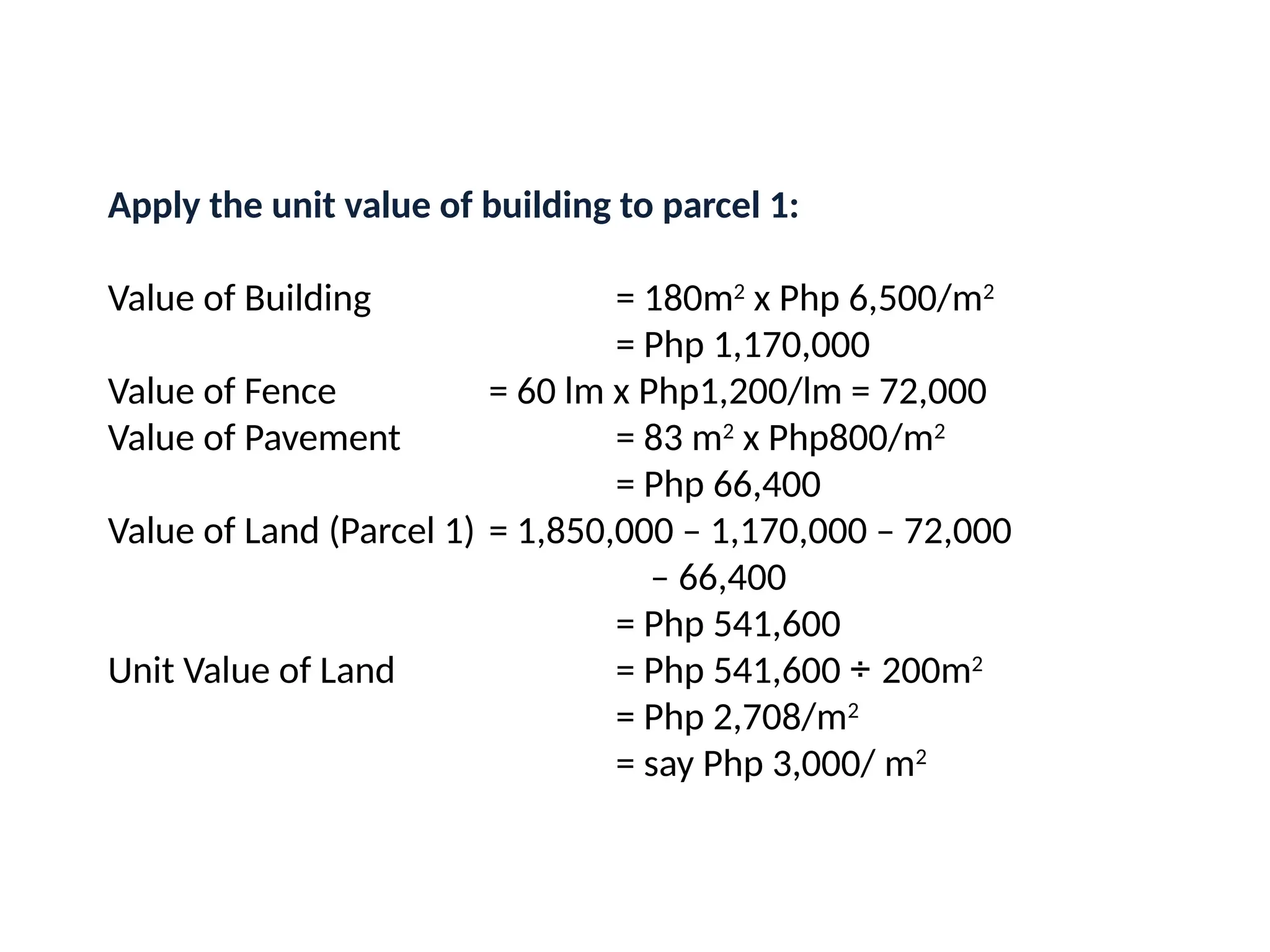

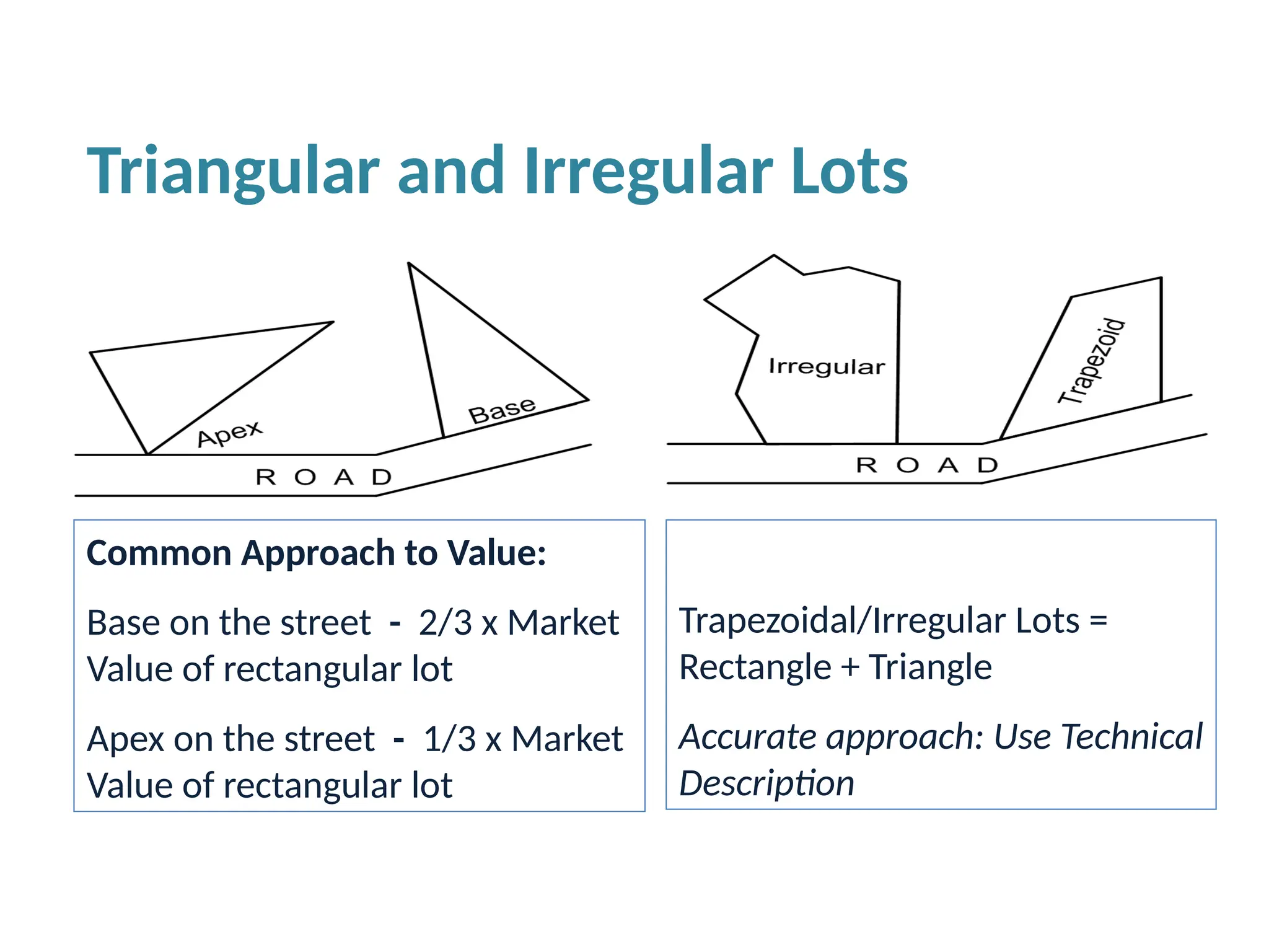
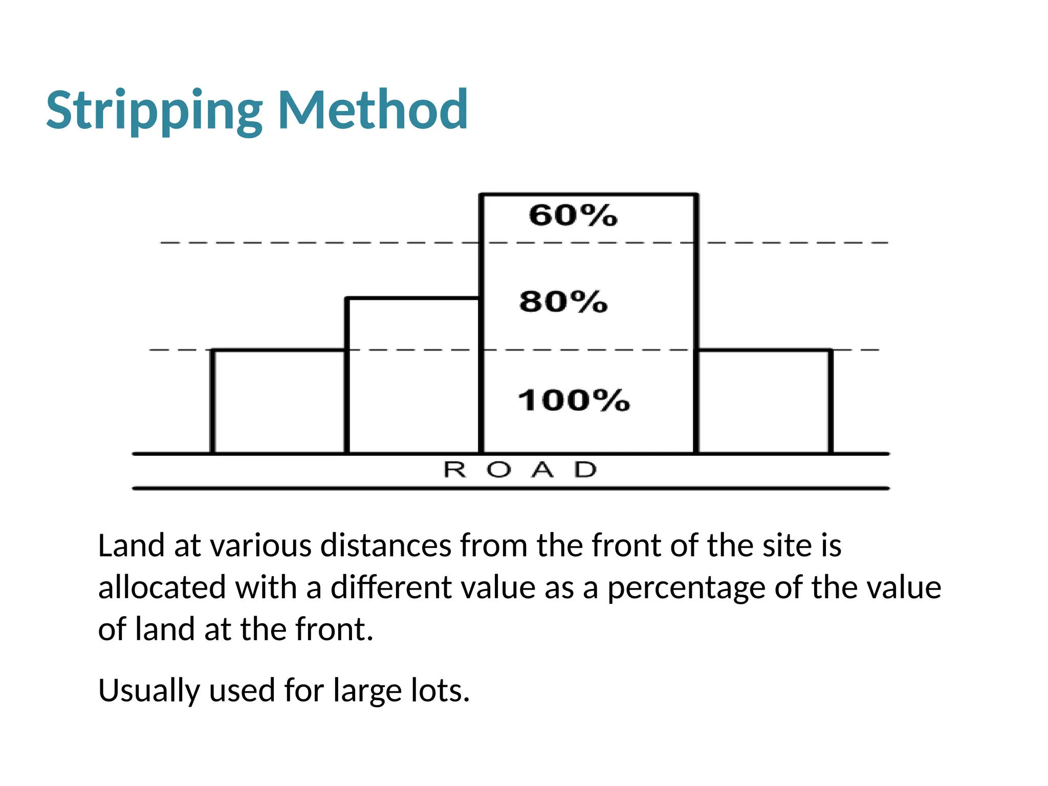
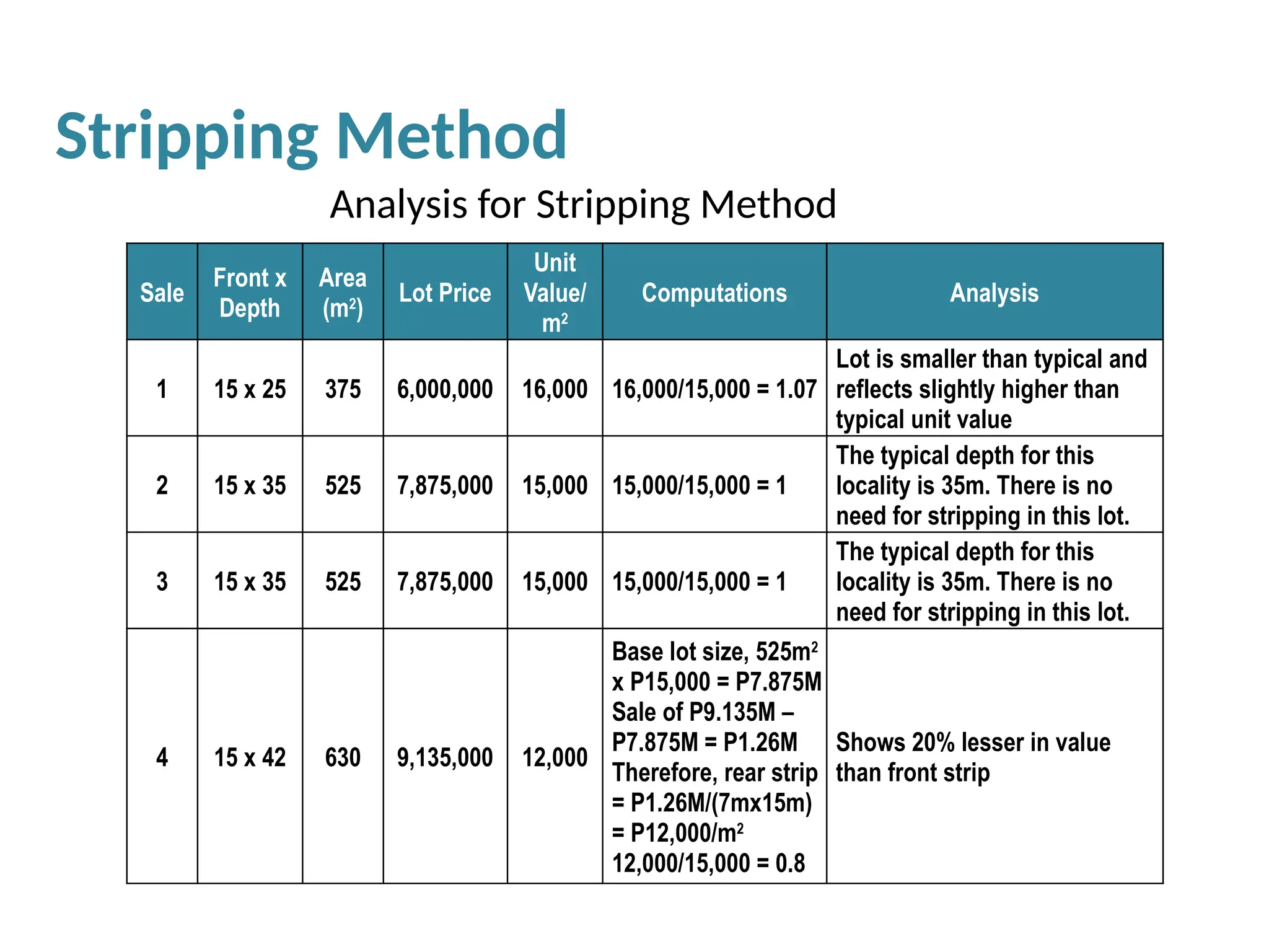
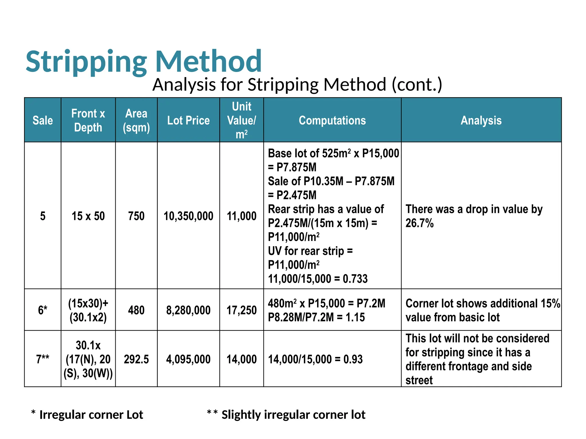
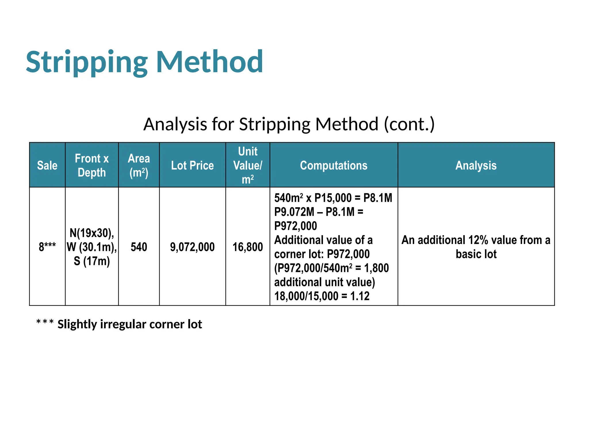
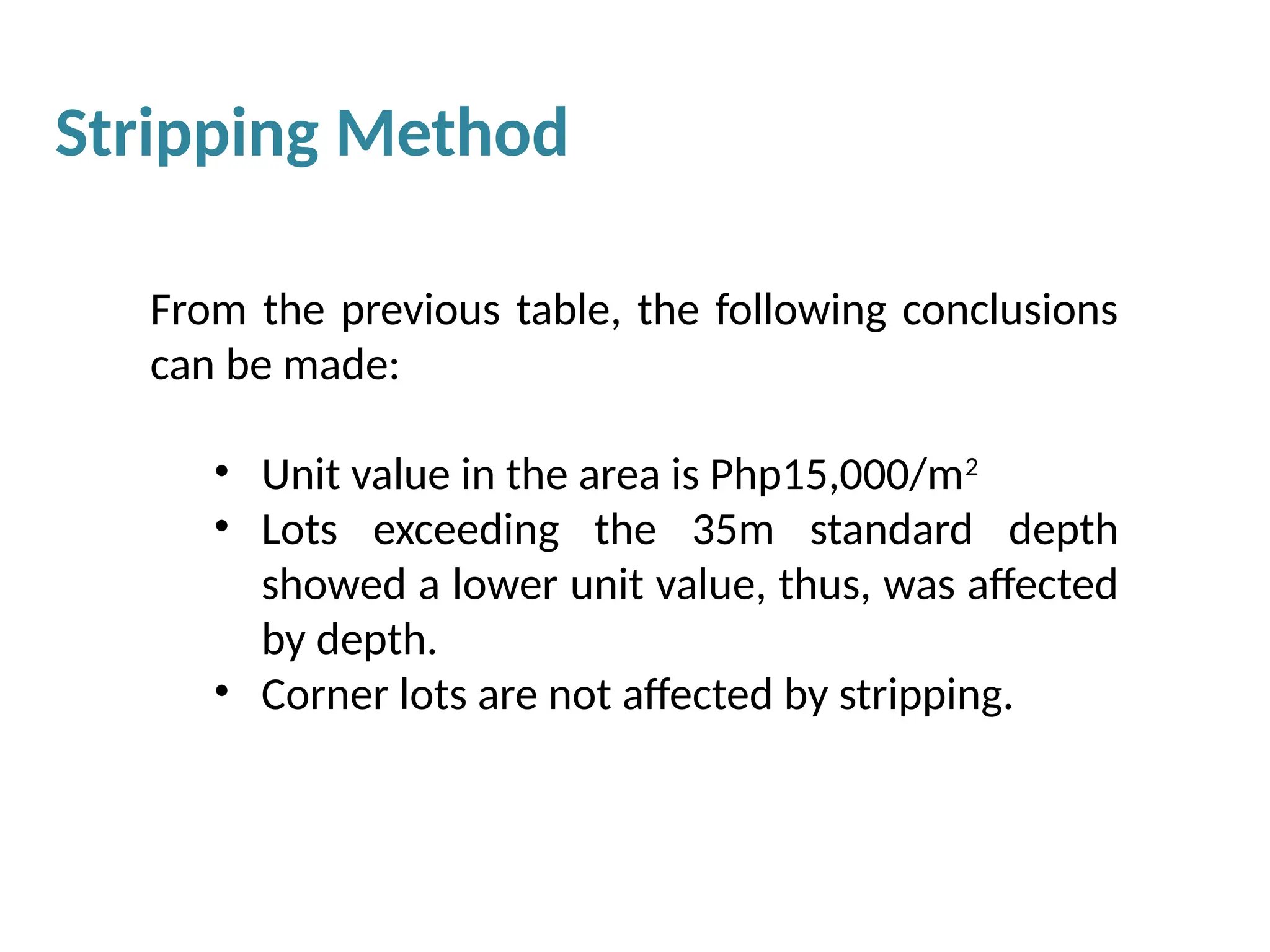
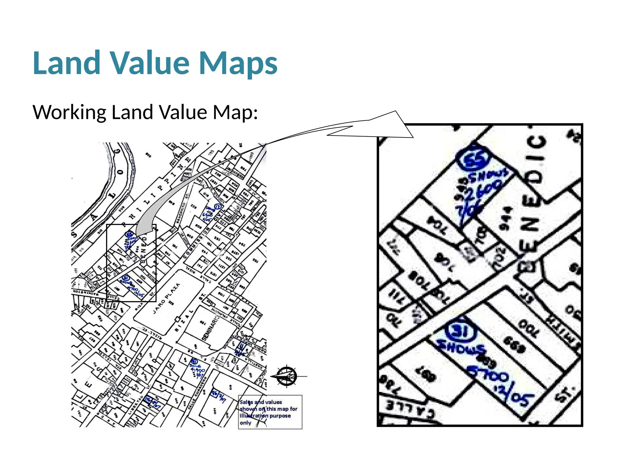
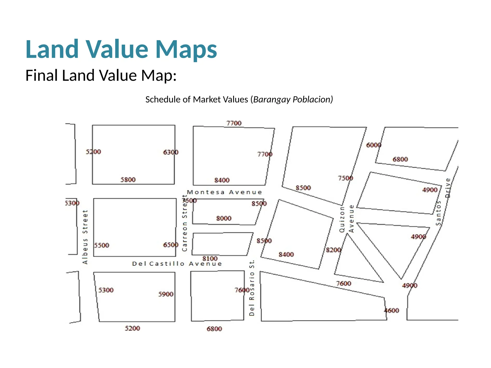

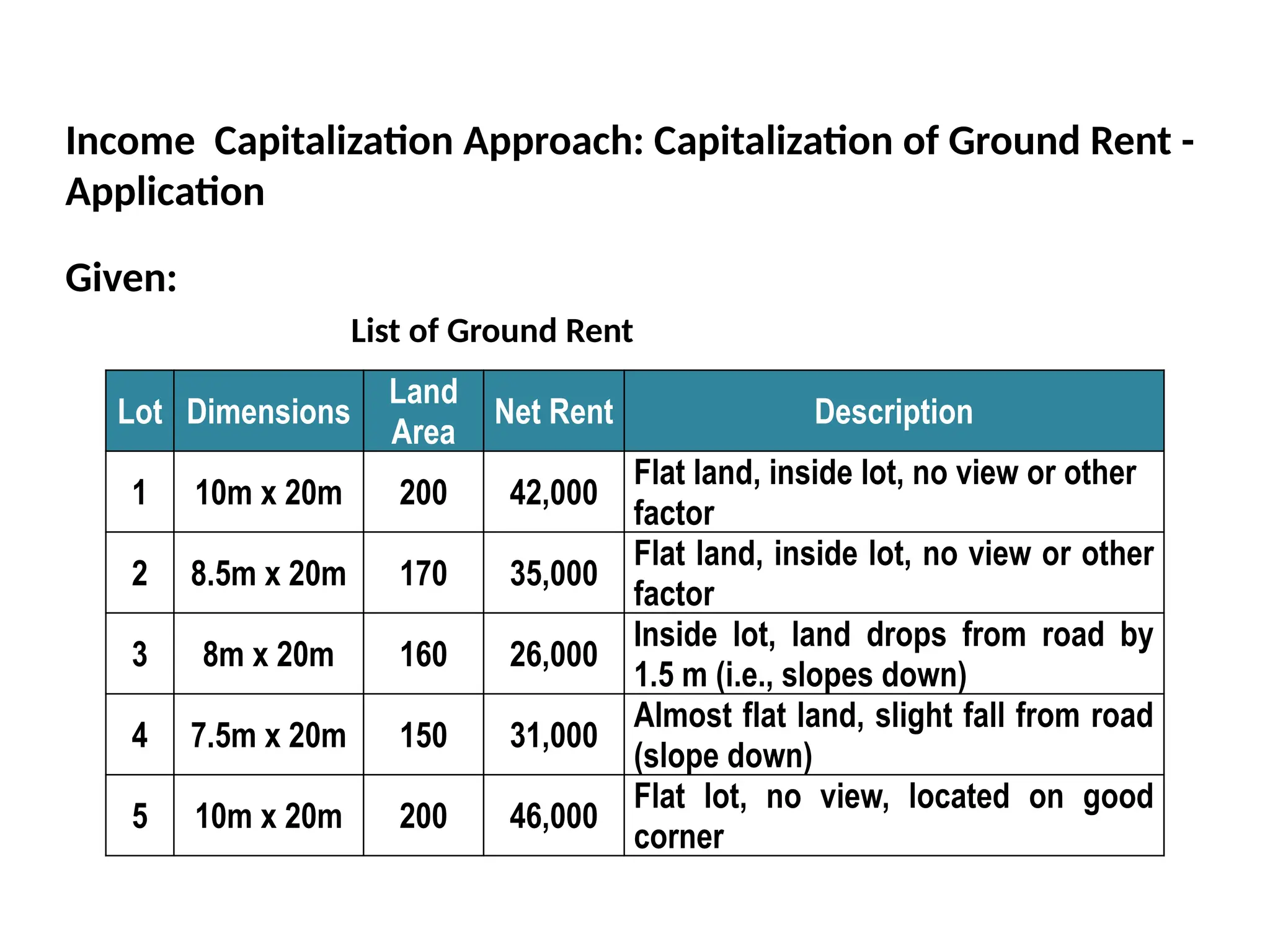
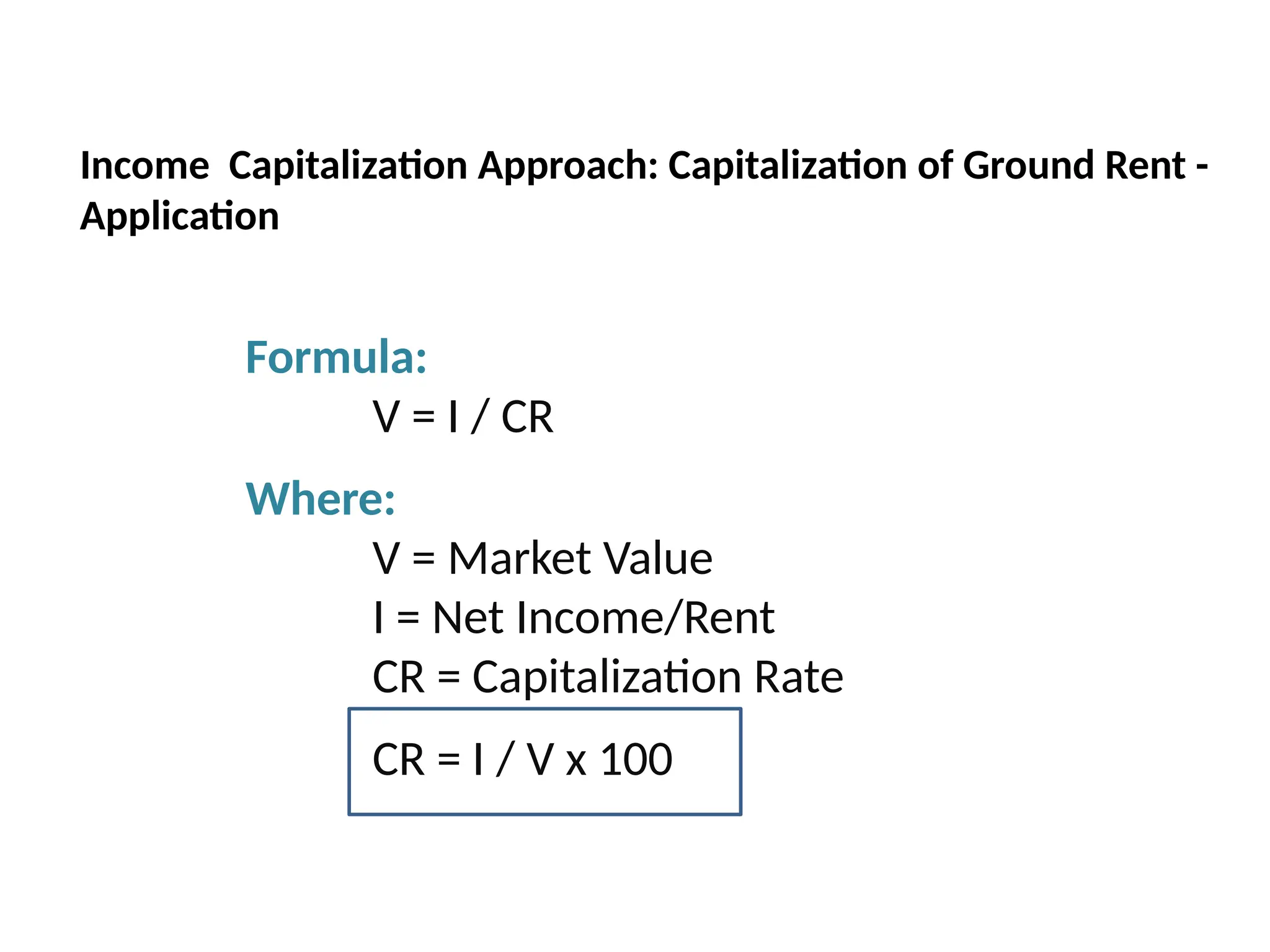

![Lot
(a)
Land
Area
(b)
Net Mo.
Rent
(c)
CR
%
(d)
Market
Value
(e)
UV
w/
Inf
(f)
Influences
(g)
Adj.
to UV
(Inf)
(h)
Unit Value
without
Influence
(i)
Rnded
Unit
Value
(j)
1 200 42,000 10 5,040,000 25,200
Flat, inside lot, no other
factor
0% 25,200 25,000
2 170 35,000 10 4,200,000 24,705
Flat, inside lot, no other
factor
0% 24,705 25,000
3 160 26,000 10 3,120,000 19,500 Inside lot, drops to 1.5m -20% 15,600 16,000
4 150 31,000 10 3,720,000 24,800 Almost flat, slight slope 0% 24,800 25,000
5 200 46,000 10 5,520,000 27,600 Flat, no view, good corner +12% 30,912 31,000
(e) = [(c)x 12)]/(d) (f) = (e)/(b) i = (f) x [(100%-(h)]/100
Income Capitalization Approach: Capitalization of Ground Rent -
Application
Determine unit values](https://image.slidesharecdn.com/module2-251125051228-3ed4c78d/75/Module-2-0Module-2-0Module-2-0-Module-2-0-pptx-144-2048.jpg)
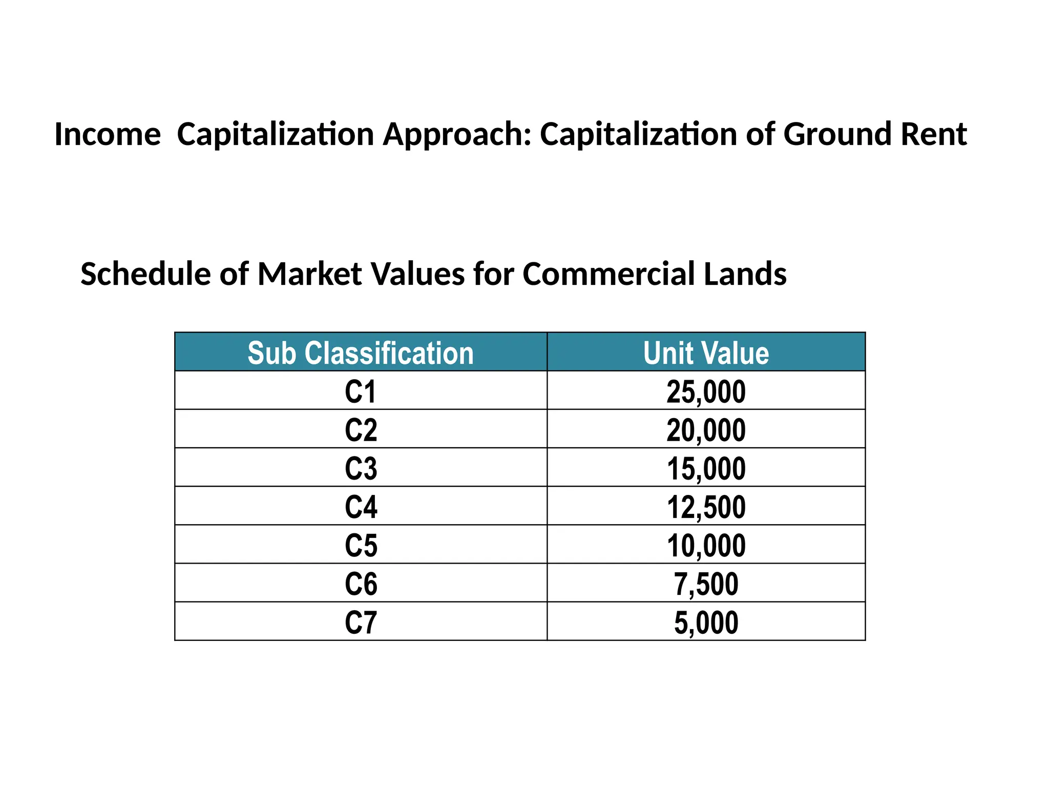
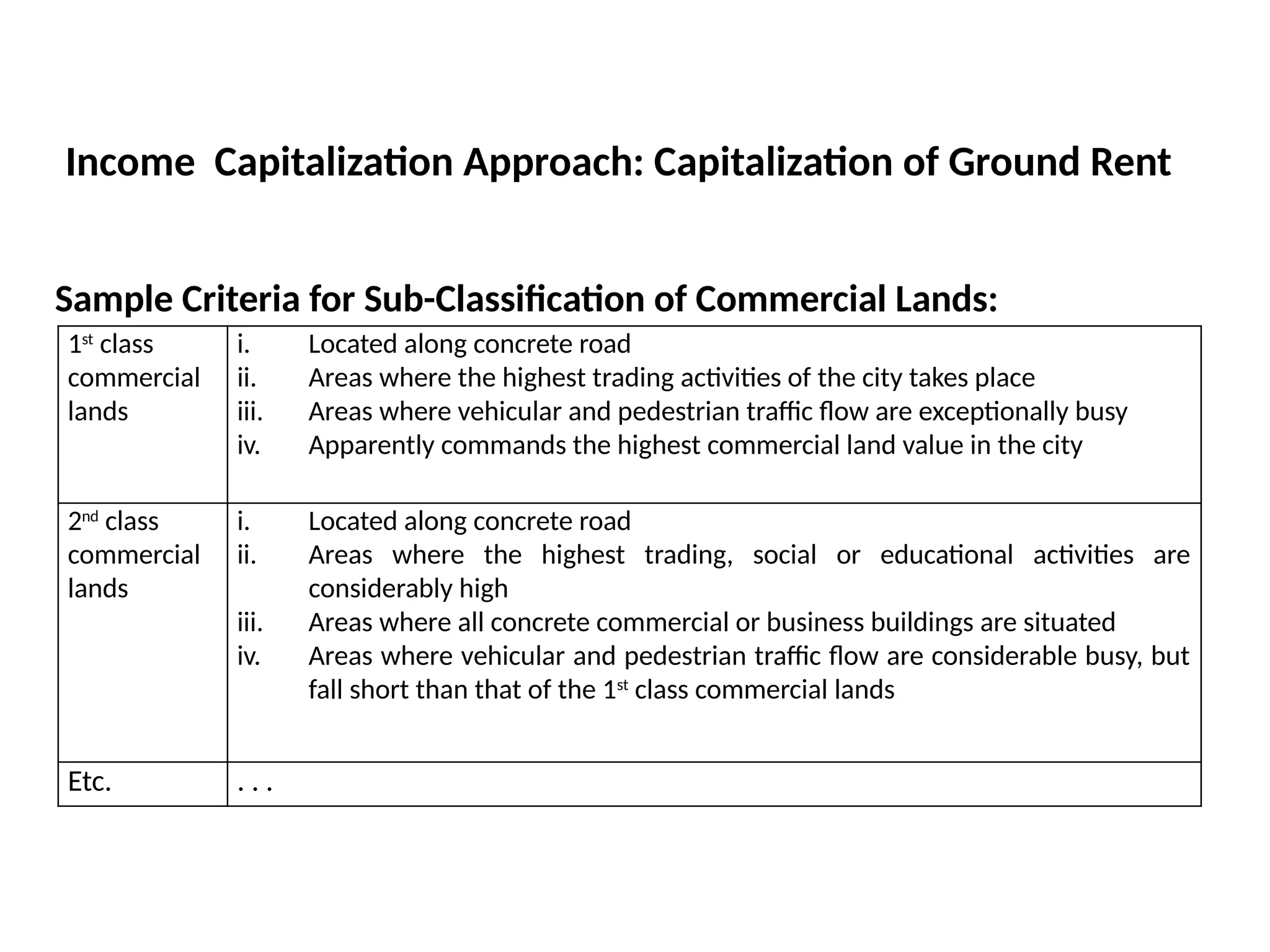
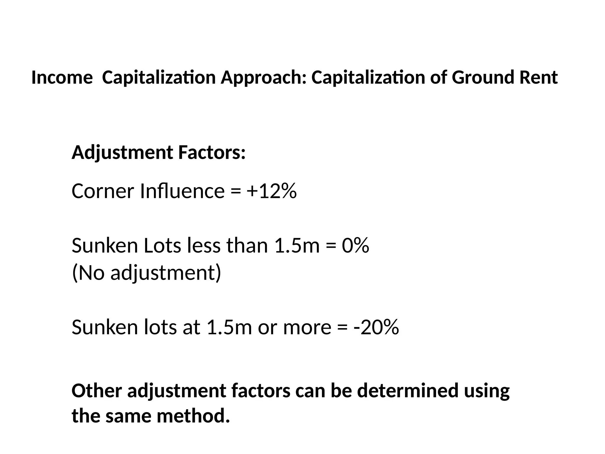
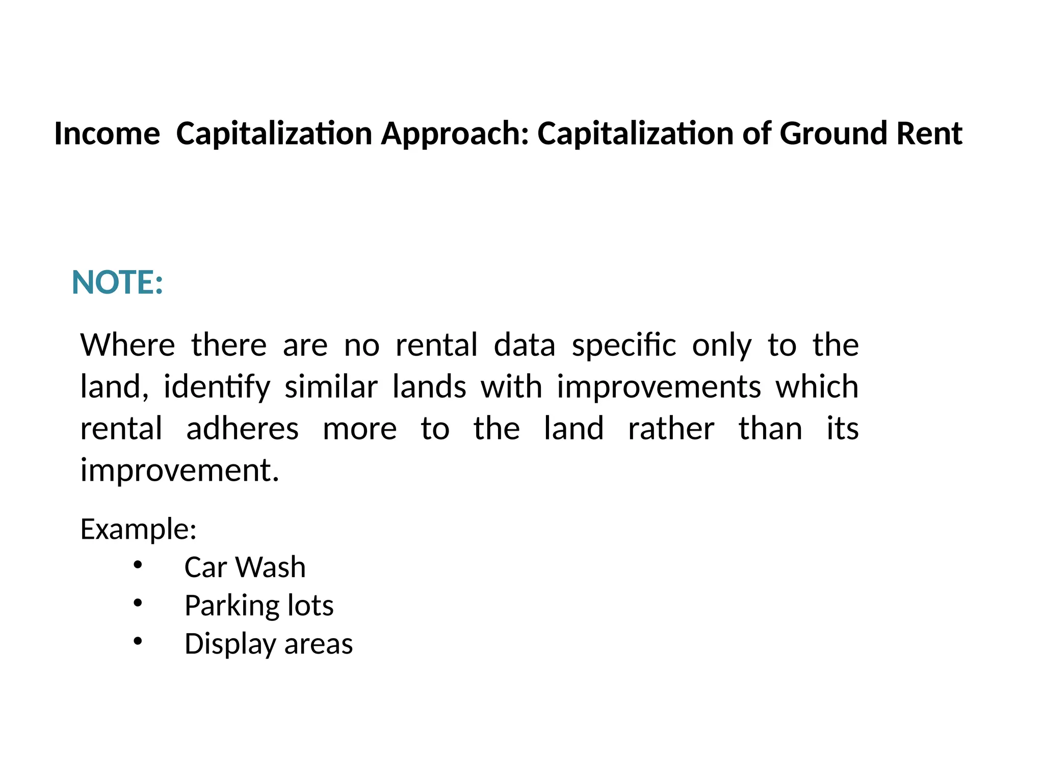
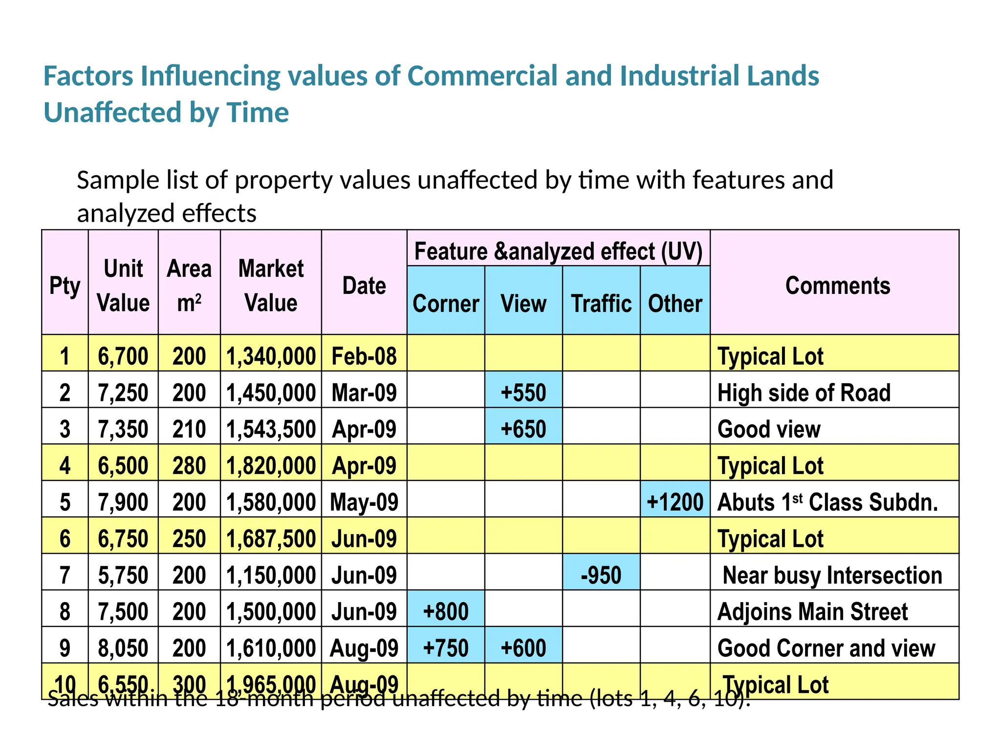
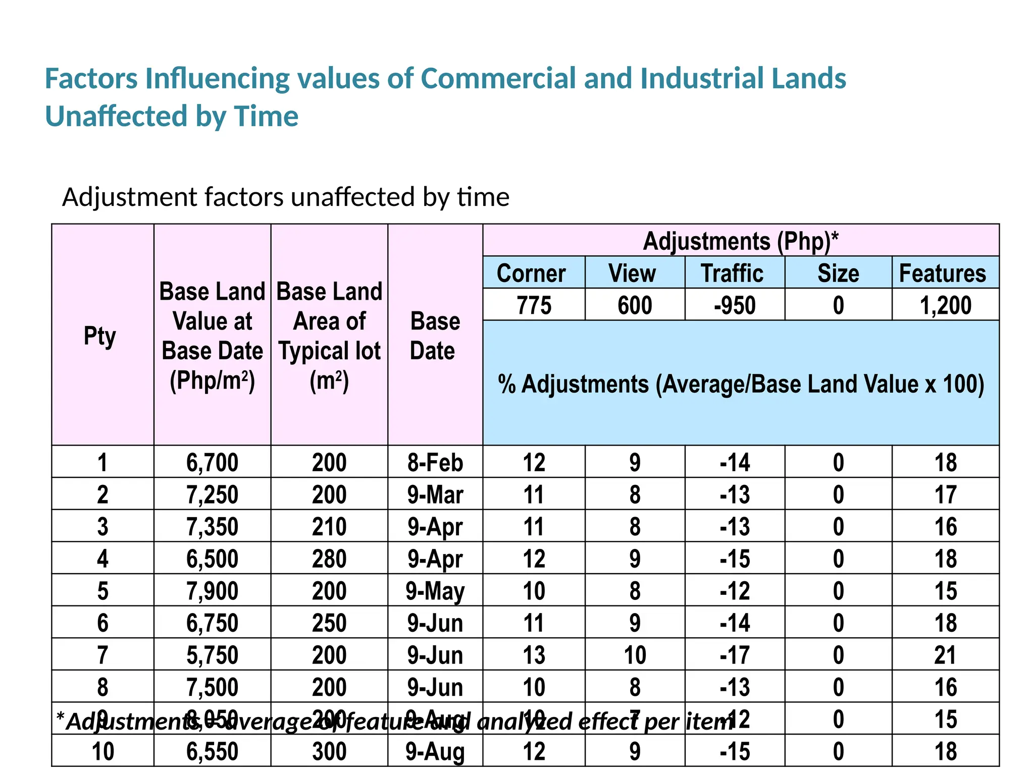
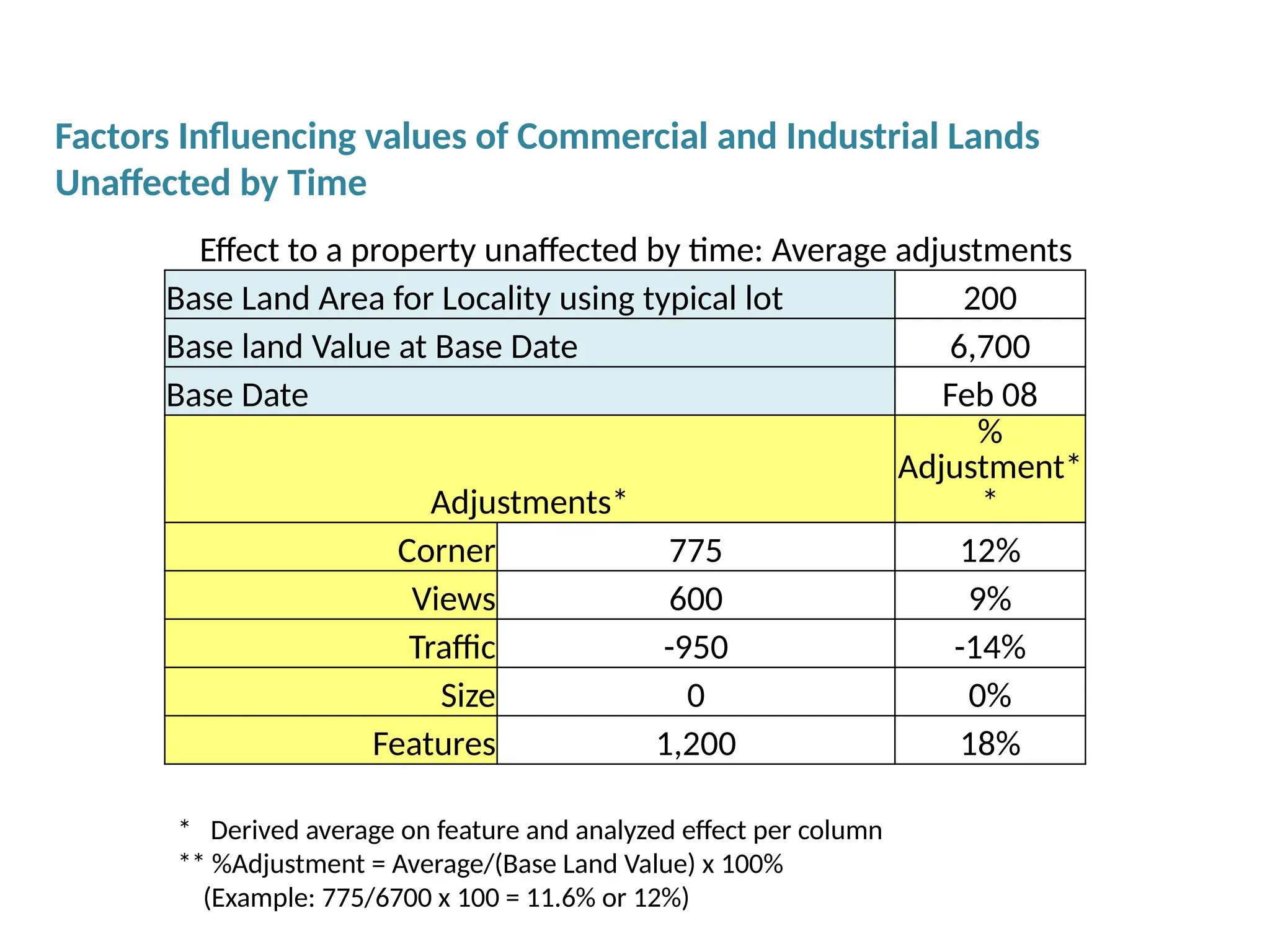
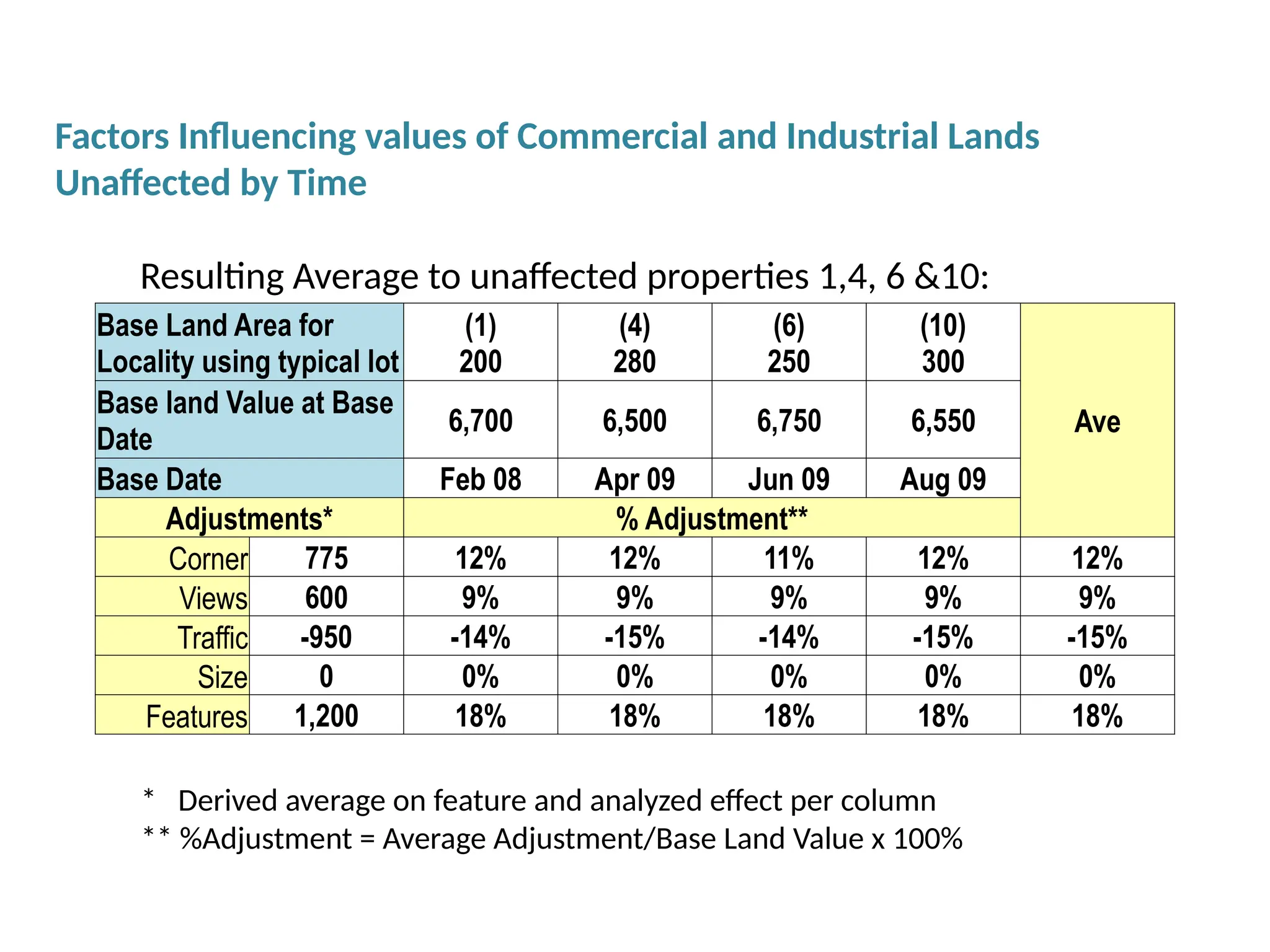
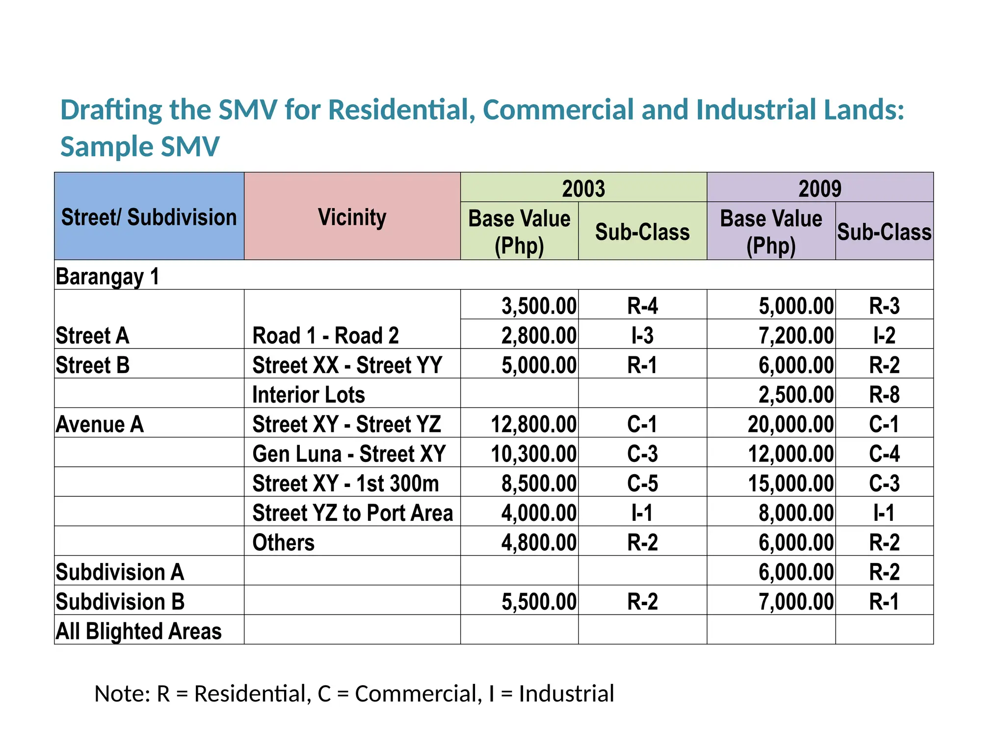


![Machinery
“Machinery embraces machines, equipment, mechanical
contrivances, instruments, appliances or apparatus, which may
not be attached, permanently or temporarily to the real
property. It includes the physical facilities for production, the
installations and appurtenant service facilities, those which are
mobile, self-powered or self-propelled, and those not
permanently attached to the real property which are actually,
directly, and exclusively used to meet the needs of the particular
industry, business or activity and which by their very nature and
purpose are designed for, or necessary to its manufacturing,
mining, logging, commercial, industrial or agricultural
purposes.”
[Local Government Code, Section 199]](https://image.slidesharecdn.com/module2-251125051228-3ed4c78d/75/Module-2-0Module-2-0Module-2-0-Module-2-0-pptx-156-2048.jpg)