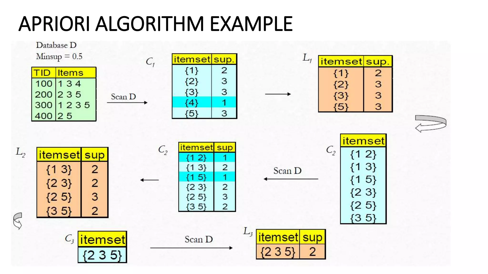
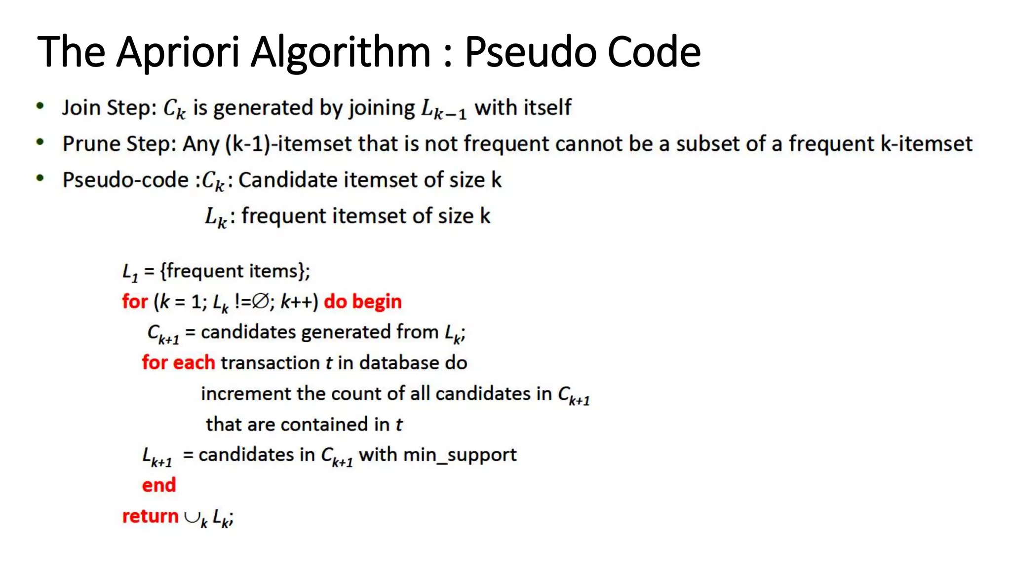
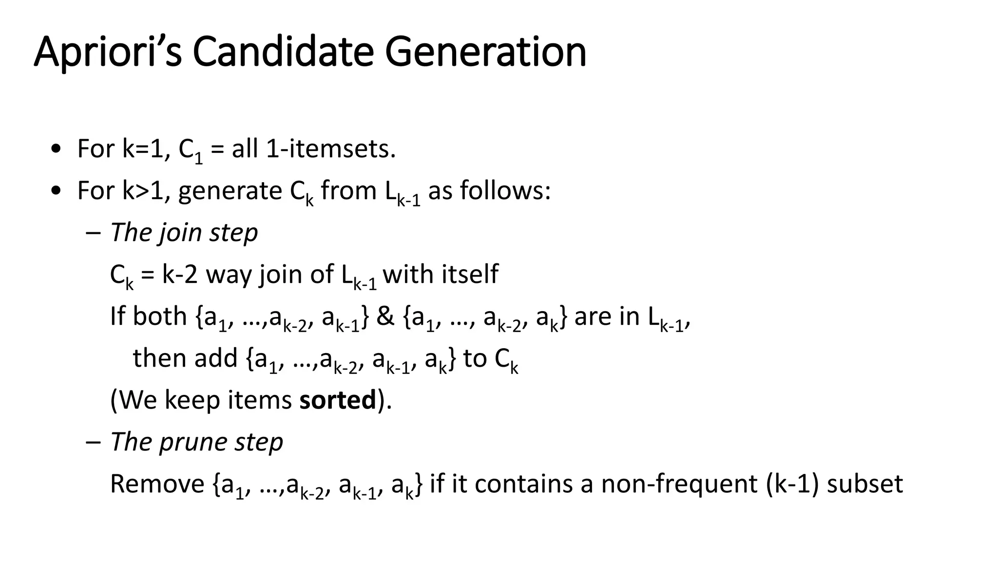
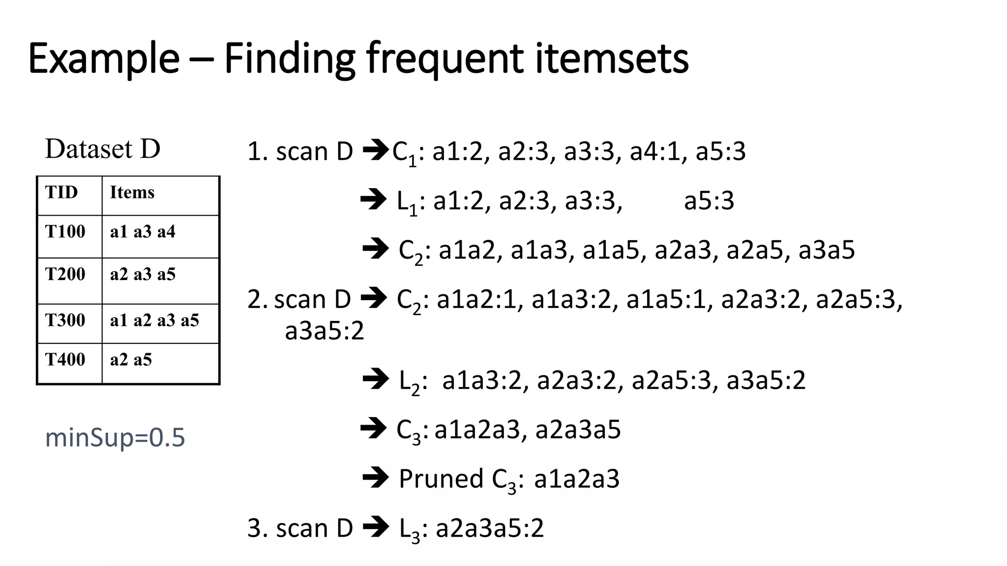
The document discusses the Apriori algorithm for mining association rules from transactional data. The Apriori algorithm uses a level-wise search where frequent itemsets are used to explore longer itemsets. It determines frequent itemsets by identifying individual frequent items and extending them to larger sets as long as they meet a minimum support threshold. The algorithm takes advantage of the fact that subsets of frequent itemsets must also be frequent to prune the search space. It performs candidate generation and pruning to efficiently identify all frequent itemsets in the transactional data.
![Association rule mining
• Proposed by Agrawal et al in 1993.
• It is an important data mining model studied extensively by the database
and data mining community.
• Assume all data are categorical.
• No good algorithm for numeric data.
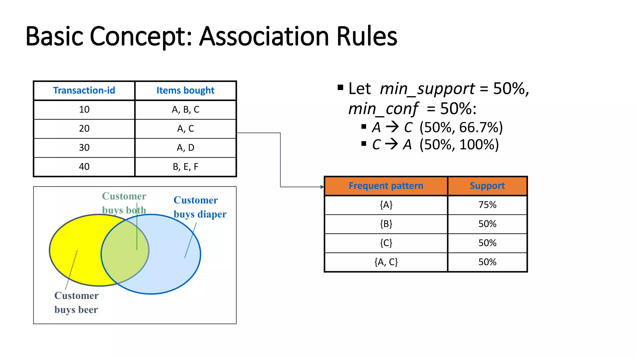
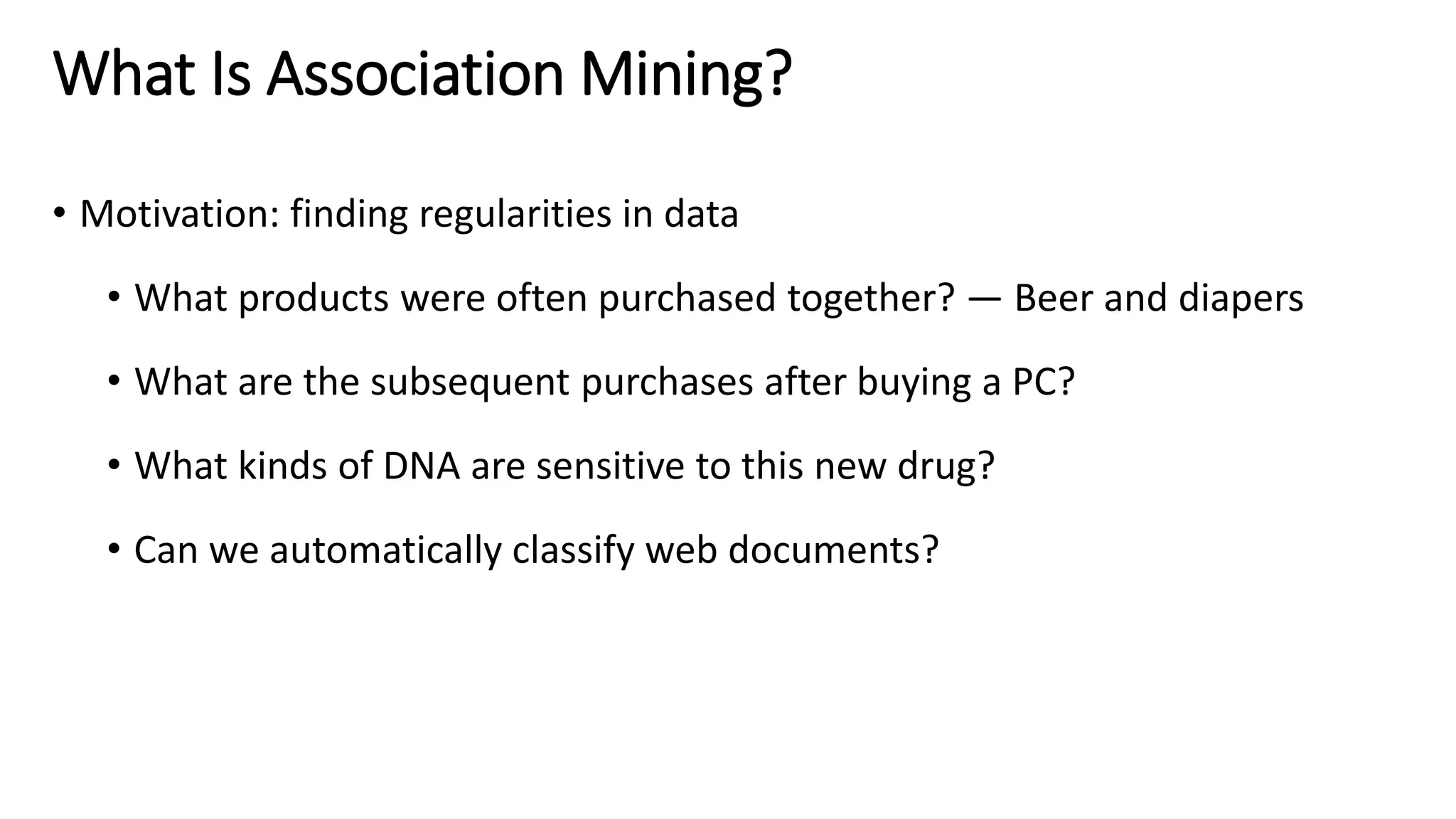
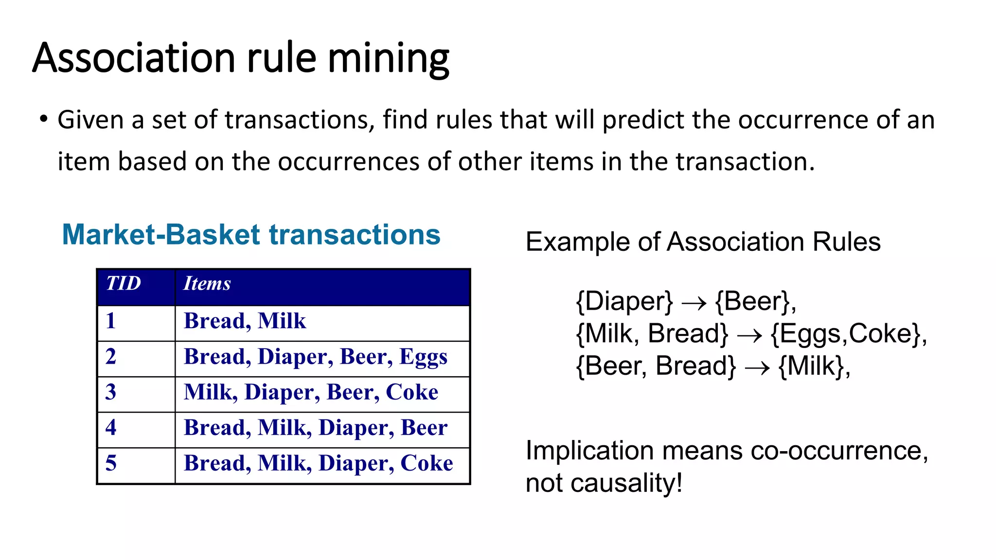
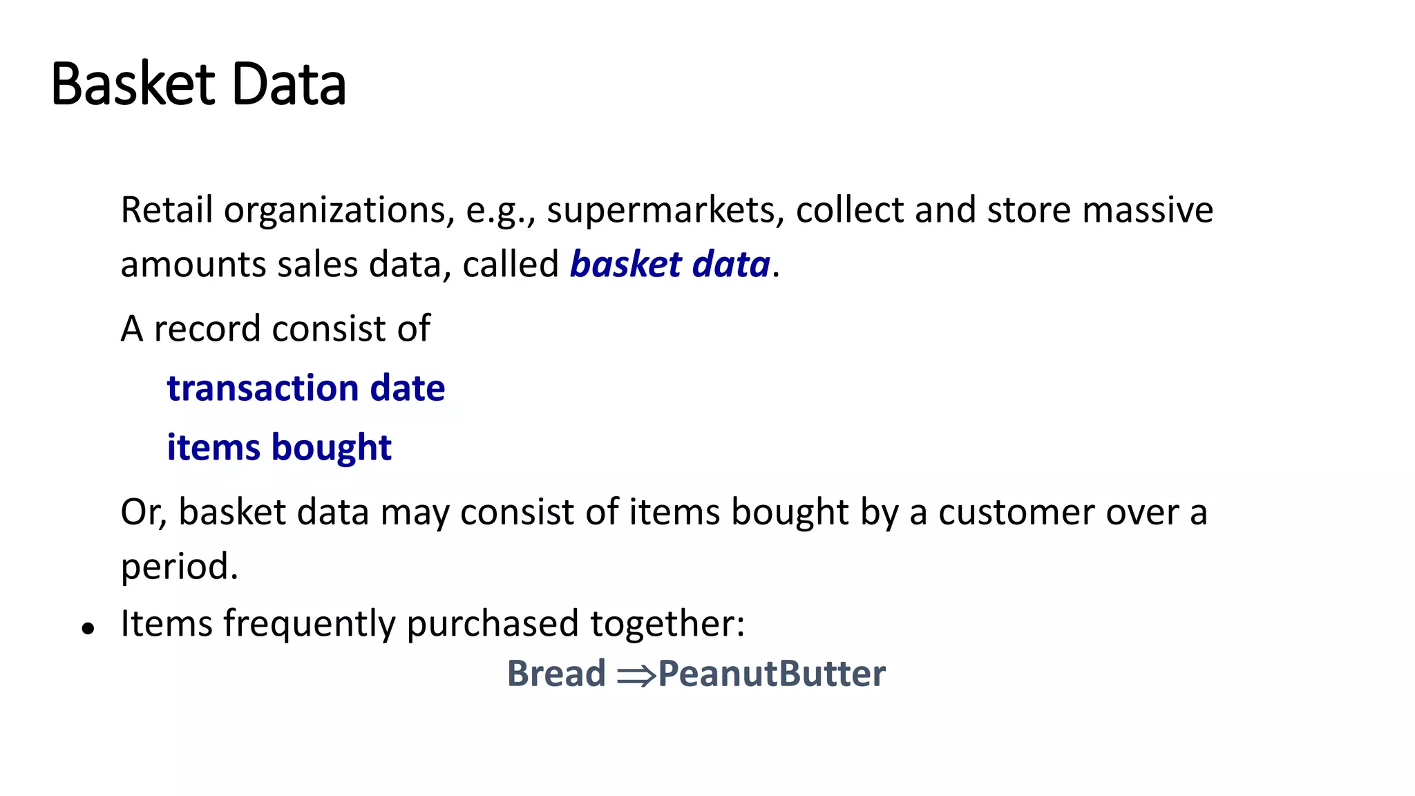
• Initially used for Market Basket Analysis to find how items purchased by
customers are related.
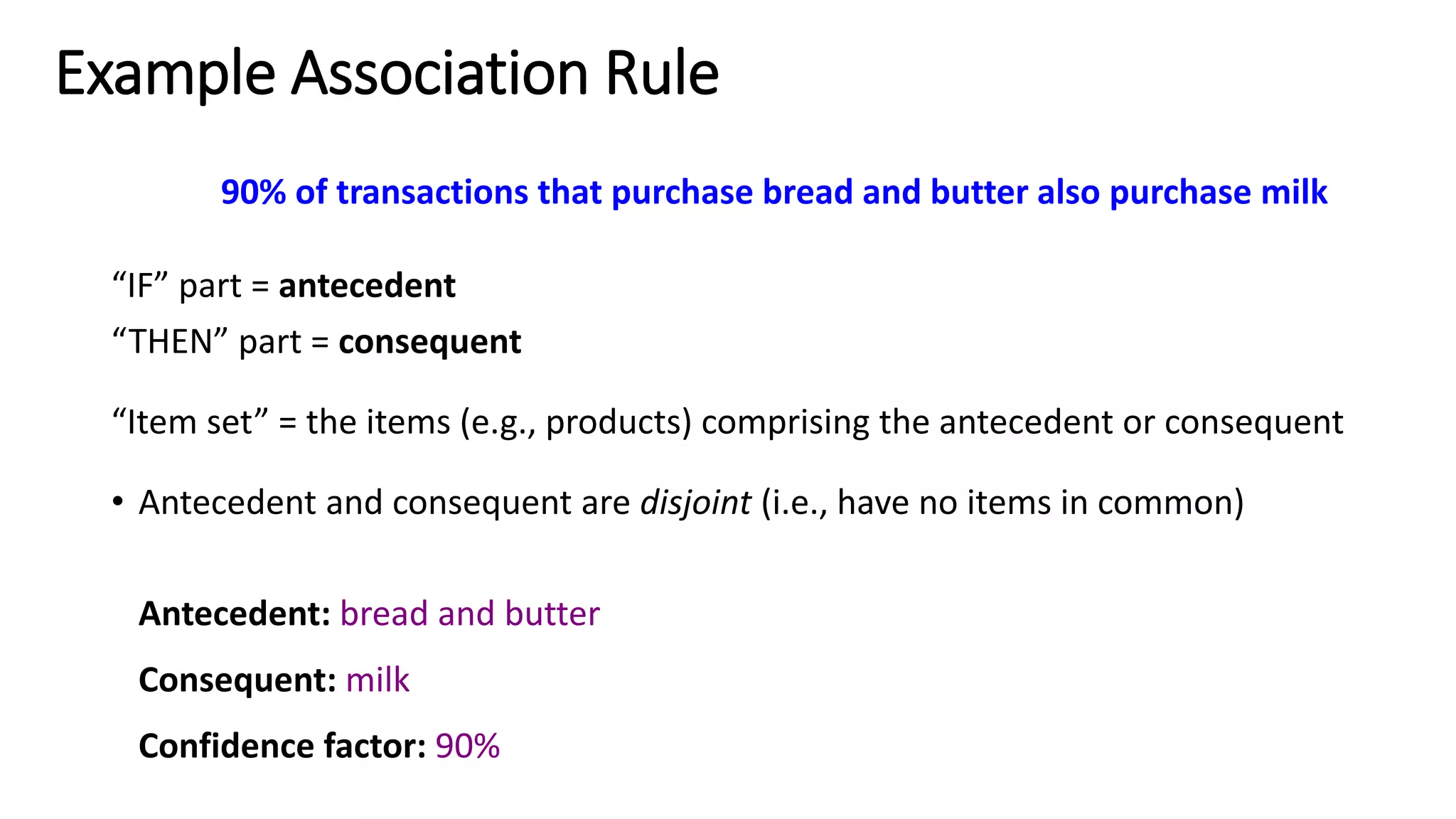
Bread Milk [sup = 5%, conf = 100%]
2](https://image.slidesharecdn.com/lect6-associationruleapriorialgorithm-190228021638/75/Lect6-Association-rule-Apriori-algorithm-2-2048.jpg)
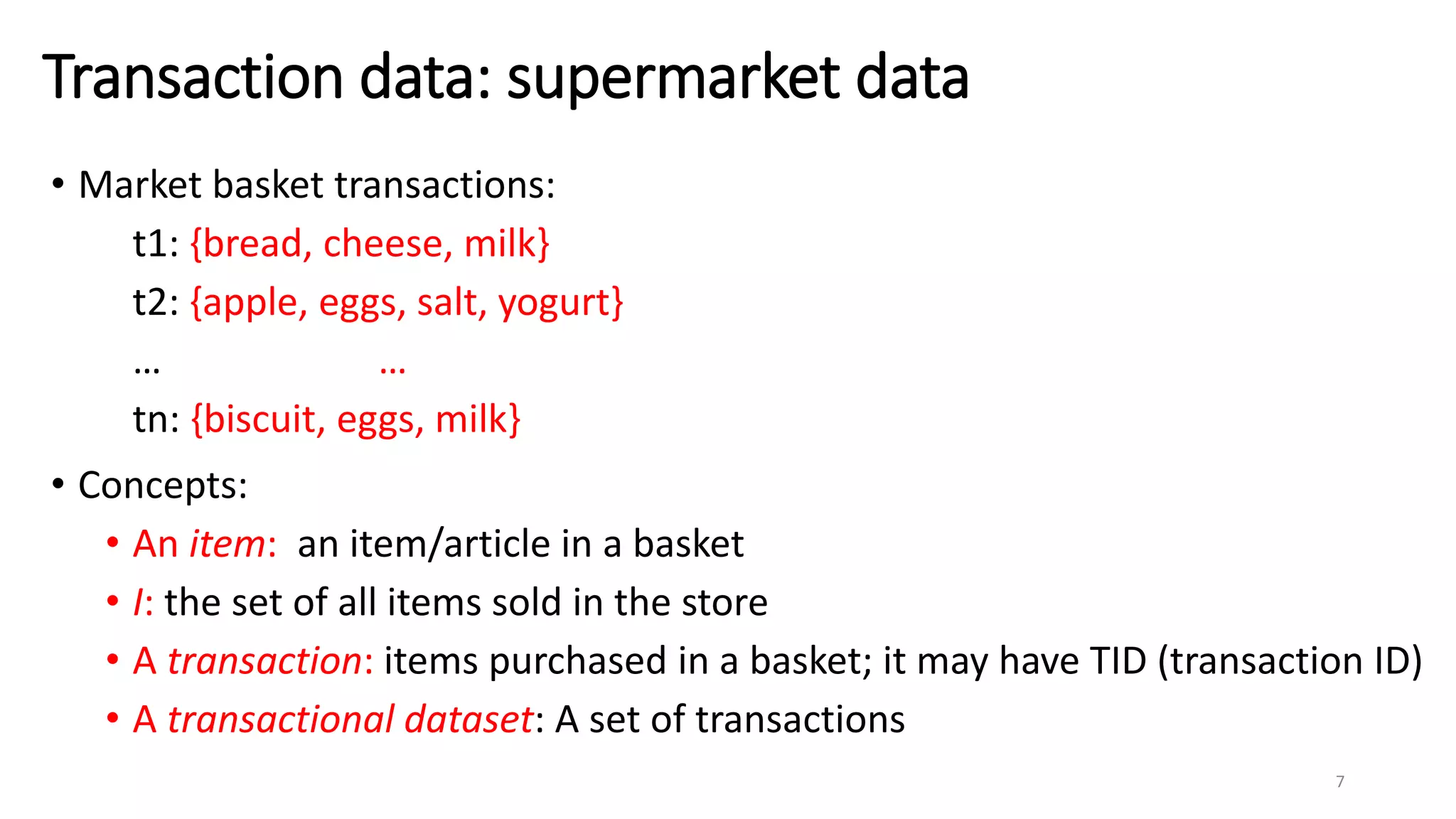
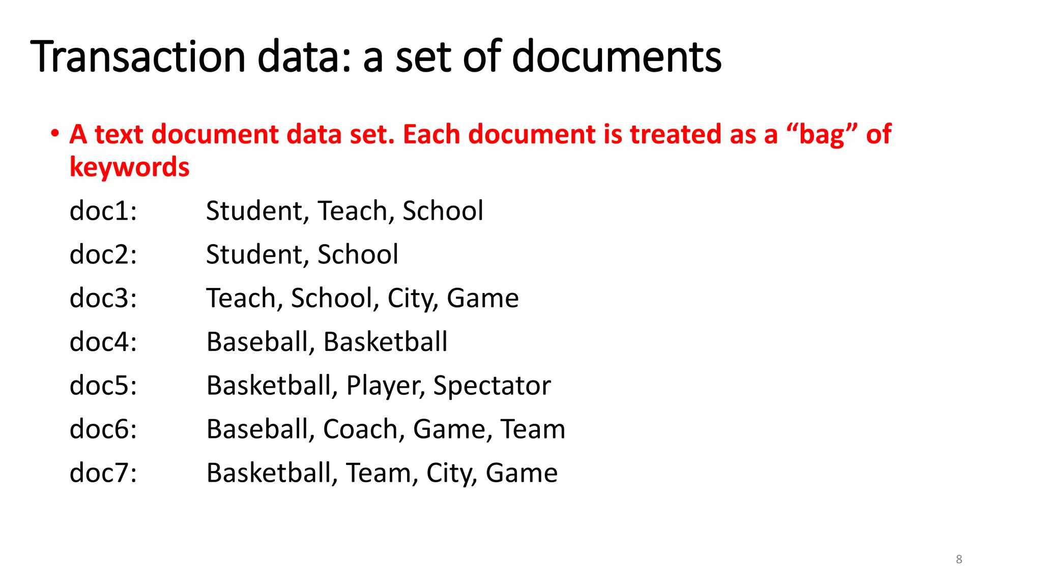
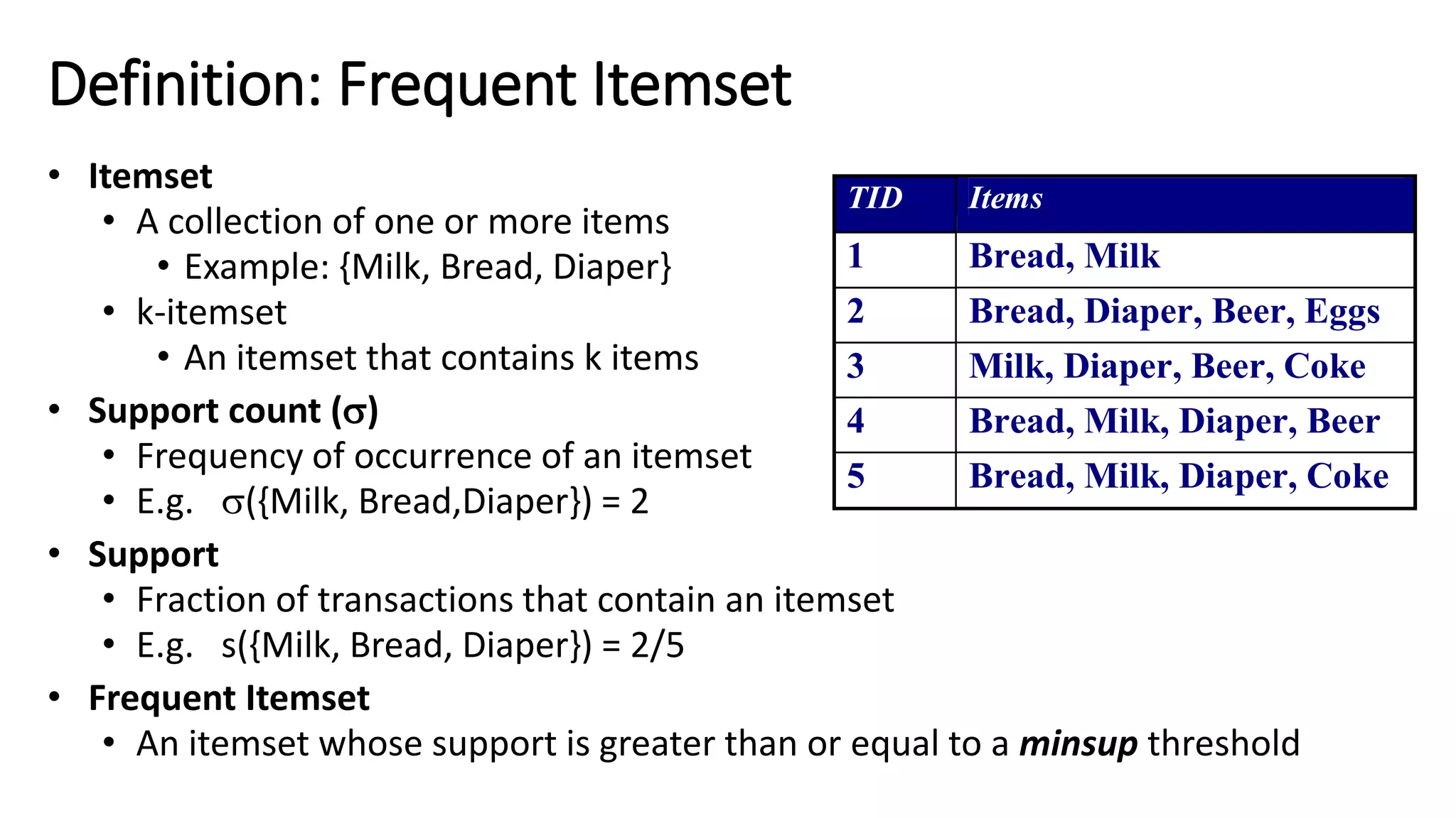
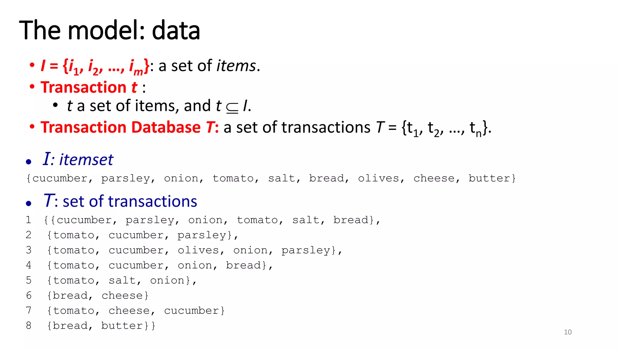
![An example
• Transaction data
• Assume:
minsup = 30%
minconf = 80%
• An example frequent itemset:
{Chicken, Clothes, Milk} [sup = 3/7]
• Association rules from the itemset:
Clothes Milk, Chicken [sup = 3/7, conf = 3/3]
… …
Clothes, Chicken Milk, [sup = 3/7, conf = 3/3]
t1: Bread, Chicken, Milk
t2: Bread, Cheese
t3: Cheese, Boots
t4: Bread, Chicken, Cheese
t5: Bread, Chicken, Clothes, Cheese, Milk
t6: Chicken, Clothes, Milk
t7: Chicken, Milk, Clothes
16](https://image.slidesharecdn.com/lect6-associationruleapriorialgorithm-190228021638/75/Lect6-Association-rule-Apriori-algorithm-16-2048.jpg)