The documents contain introduction to optimization methods which is very usefu for reseachers and other students
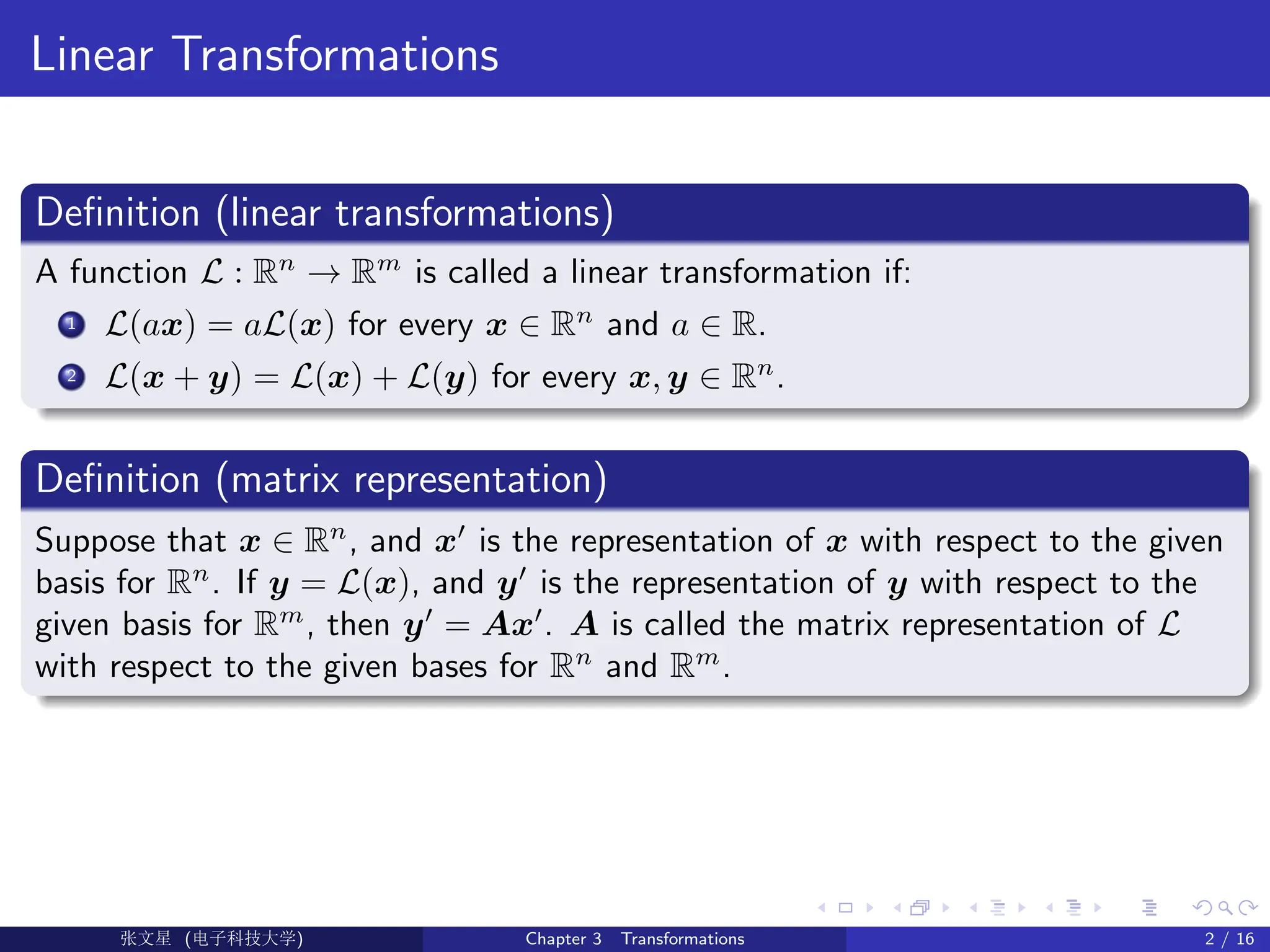
![Linear Transformations
Definition (transformation matrix)
Let {e1, e2, . . . , en} and {e0
1, e0
2, . . . , e0
n} be two bases for Rn
. Define the matrix
T = [e0
1, e0
2, . . . , e0
n]−1
[e1, e2, . . . , en], or equivalently
[e1, e2, . . . , en] = [e0
1, e0
2, . . . , e0
n]T ,
T is called the transformation matrix.
Ü©( (>f‰EŒÆ) Chapter 3 Transformations 3 / 16](https://image.slidesharecdn.com/chapter3-251114130840-87080d8d/75/Introduction-to-Optimization-methods-lecture-1-7-2048.jpg)
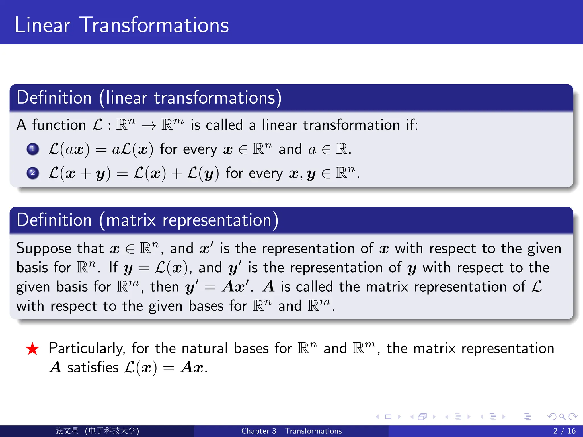
![Linear Transformations
Definition (transformation matrix)
Let {e1, e2, . . . , en} and {e0
1, e0
2, . . . , e0
n} be two bases for Rn
. Define the matrix
T = [e0
1, e0
2, . . . , e0
n]−1
[e1, e2, . . . , en], or equivalently
[e1, e2, . . . , en] = [e0
1, e0
2, . . . , e0
n]T ,
T is called the transformation matrix.
Example
For any u ∈ Rn
, let x (resp. x0
) be the coordinates of u with respect to
{e1, e2, . . . , en} (resp. {e0
1, e0
2, . . . , e0
n}). Then, x0
= T x.
Ü©( (>f‰EŒÆ) Chapter 3 Transformations 3 / 16](https://image.slidesharecdn.com/chapter3-251114130840-87080d8d/75/Introduction-to-Optimization-methods-lecture-1-8-2048.jpg)
![Linear Transformations
Definition (transformation matrix)
Let {e1, e2, . . . , en} and {e0
1, e0
2, . . . , e0
n} be two bases for Rn
. Define the matrix
T = [e0
1, e0
2, . . . , e0
n]−1
[e1, e2, . . . , en], or equivalently
[e1, e2, . . . , en] = [e0
1, e0
2, . . . , e0
n]T ,
T is called the transformation matrix.
Example
For any u ∈ Rn
, let x (resp. x0
) be the coordinates of u with respect to
{e1, e2, . . . , en} (resp. {e0
1, e0
2, . . . , e0
n}). Then, x0
= T x.
Similarity: A linear transformation L : Rn
→ Rm
.
Ü©( (>f‰EŒÆ) Chapter 3 Transformations 3 / 16](https://image.slidesharecdn.com/chapter3-251114130840-87080d8d/75/Introduction-to-Optimization-methods-lecture-1-9-2048.jpg)
![Linear Transformations
Definition (transformation matrix)
Let {e1, e2, . . . , en} and {e0
1, e0
2, . . . , e0
n} be two bases for Rn
. Define the matrix
T = [e0
1, e0
2, . . . , e0
n]−1
[e1, e2, . . . , en], or equivalently
[e1, e2, . . . , en] = [e0
1, e0
2, . . . , e0
n]T ,
T is called the transformation matrix.
Example
For any u ∈ Rn
, let x (resp. x0
) be the coordinates of u with respect to
{e1, e2, . . . , en} (resp. {e0
1, e0
2, . . . , e0
n}). Then, x0
= T x.
Similarity: A linear transformation L : Rn
→ Rm
.
Let A (resp. B) be its representation of {e1, e2, . . . , en} (resp. {e0
1, e0
2, . . . , e0
n}).
Ü©( (>f‰EŒÆ) Chapter 3 Transformations 3 / 16](https://image.slidesharecdn.com/chapter3-251114130840-87080d8d/75/Introduction-to-Optimization-methods-lecture-1-10-2048.jpg)
![Linear Transformations
Definition (transformation matrix)
Let {e1, e2, . . . , en} and {e0
1, e0
2, . . . , e0
n} be two bases for Rn
. Define the matrix
T = [e0
1, e0
2, . . . , e0
n]−1
[e1, e2, . . . , en], or equivalently
[e1, e2, . . . , en] = [e0
1, e0
2, . . . , e0
n]T ,
T is called the transformation matrix.
Example
For any u ∈ Rn
, let x (resp. x0
) be the coordinates of u with respect to
{e1, e2, . . . , en} (resp. {e0
1, e0
2, . . . , e0
n}). Then, x0
= T x.
Similarity: A linear transformation L : Rn
→ Rm
.
Let A (resp. B) be its representation of {e1, e2, . . . , en} (resp. {e0
1, e0
2, . . . , e0
n}).
Let y = Ax and y0
= Bx0
.
Ü©( (>f‰EŒÆ) Chapter 3 Transformations 3 / 16](https://image.slidesharecdn.com/chapter3-251114130840-87080d8d/75/Introduction-to-Optimization-methods-lecture-1-11-2048.jpg)
![Linear Transformations
Definition (transformation matrix)
Let {e1, e2, . . . , en} and {e0
1, e0
2, . . . , e0
n} be two bases for Rn
. Define the matrix
T = [e0
1, e0
2, . . . , e0
n]−1
[e1, e2, . . . , en], or equivalently
[e1, e2, . . . , en] = [e0
1, e0
2, . . . , e0
n]T ,
T is called the transformation matrix.
Example
For any u ∈ Rn
, let x (resp. x0
) be the coordinates of u with respect to
{e1, e2, . . . , en} (resp. {e0
1, e0
2, . . . , e0
n}). Then, x0
= T x.
Similarity: A linear transformation L : Rn
→ Rm
.
Let A (resp. B) be its representation of {e1, e2, . . . , en} (resp. {e0
1, e0
2, . . . , e0
n}).
Let y = Ax and y0
= Bx0
.
∴ y0
= T y = T Ax = Bx0
= BT x,
Ü©( (>f‰EŒÆ) Chapter 3 Transformations 3 / 16](https://image.slidesharecdn.com/chapter3-251114130840-87080d8d/75/Introduction-to-Optimization-methods-lecture-1-12-2048.jpg)
![Linear Transformations
Definition (transformation matrix)
Let {e1, e2, . . . , en} and {e0
1, e0
2, . . . , e0
n} be two bases for Rn
. Define the matrix
T = [e0
1, e0
2, . . . , e0
n]−1
[e1, e2, . . . , en], or equivalently
[e1, e2, . . . , en] = [e0
1, e0
2, . . . , e0
n]T ,
T is called the transformation matrix.
Example
For any u ∈ Rn
, let x (resp. x0
) be the coordinates of u with respect to
{e1, e2, . . . , en} (resp. {e0
1, e0
2, . . . , e0
n}). Then, x0
= T x.
Similarity: A linear transformation L : Rn
→ Rm
.
Let A (resp. B) be its representation of {e1, e2, . . . , en} (resp. {e0
1, e0
2, . . . , e0
n}).
Let y = Ax and y0
= Bx0
.
∴ y0
= T y = T Ax = Bx0
= BT x,
hence, T A = BT , or A = T −1
BT .
Ü©( (>f‰EŒÆ) Chapter 3 Transformations 3 / 16](https://image.slidesharecdn.com/chapter3-251114130840-87080d8d/75/Introduction-to-Optimization-methods-lecture-1-13-2048.jpg)
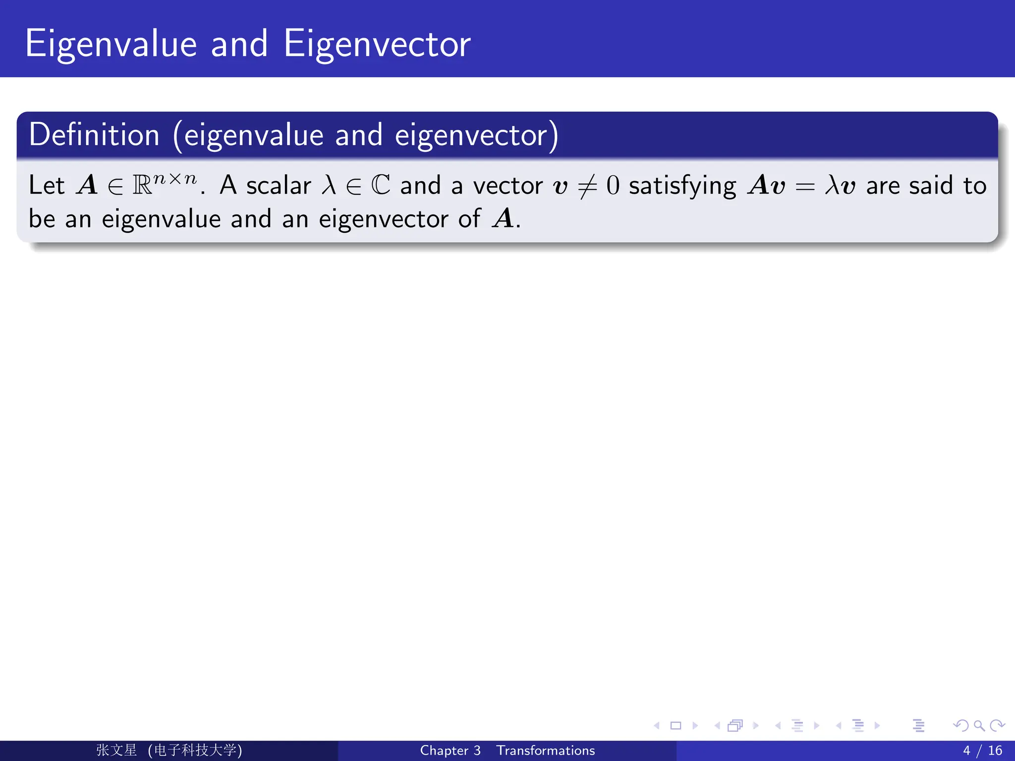
![Eigenvalue and Eigenvector
Definition (eigenvalue and eigenvector)
Let A ∈ Rn×n
. A scalar λ ∈ C and a vector v 6= 0 satisfying Av = λv are said to
be an eigenvalue and an eigenvector of A.
F Calculation of eigenvalues/spectrum of A ⇐⇒
det[λI − A] = λn
+ an−1λn−1
+ · · · + a1λ + a0 = 0. (characteristic equation)
Ü©( (>f‰EŒÆ) Chapter 3 Transformations 4 / 16](https://image.slidesharecdn.com/chapter3-251114130840-87080d8d/75/Introduction-to-Optimization-methods-lecture-1-15-2048.jpg)
![Eigenvalue and Eigenvector
Definition (eigenvalue and eigenvector)
Let A ∈ Rn×n
. A scalar λ ∈ C and a vector v 6= 0 satisfying Av = λv are said to
be an eigenvalue and an eigenvector of A.
F Calculation of eigenvalues/spectrum of A ⇐⇒
det[λI − A] = λn
+ an−1λn−1
+ · · · + a1λ + a0 = 0. (characteristic equation)
Corollary
If det[λI − A] = 0 has n distinct roots {λi}n
i=1. Then, there exist n linearly
independent vectors {vi}n
i=1 such that Avi = λivi, i = 1, . . . , n.
Ü©( (>f‰EŒÆ) Chapter 3 Transformations 4 / 16](https://image.slidesharecdn.com/chapter3-251114130840-87080d8d/75/Introduction-to-Optimization-methods-lecture-1-16-2048.jpg)
![Eigenvalue and Eigenvector
Definition (eigenvalue and eigenvector)
Let A ∈ Rn×n
. A scalar λ ∈ C and a vector v 6= 0 satisfying Av = λv are said to
be an eigenvalue and an eigenvector of A.
F Calculation of eigenvalues/spectrum of A ⇐⇒
det[λI − A] = λn
+ an−1λn−1
+ · · · + a1λ + a0 = 0. (characteristic equation)
Corollary
If det[λI − A] = 0 has n distinct roots {λi}n
i=1. Then, there exist n linearly
independent vectors {vi}n
i=1 such that Avi = λivi, i = 1, . . . , n.
Theorem (let A ∈ Rn×n
be a square matrix)
Ü©( (>f‰EŒÆ) Chapter 3 Transformations 4 / 16](https://image.slidesharecdn.com/chapter3-251114130840-87080d8d/75/Introduction-to-Optimization-methods-lecture-1-17-2048.jpg)
![Eigenvalue and Eigenvector
Definition (eigenvalue and eigenvector)
Let A ∈ Rn×n
. A scalar λ ∈ C and a vector v 6= 0 satisfying Av = λv are said to
be an eigenvalue and an eigenvector of A.
F Calculation of eigenvalues/spectrum of A ⇐⇒
det[λI − A] = λn
+ an−1λn−1
+ · · · + a1λ + a0 = 0. (characteristic equation)
Corollary
If det[λI − A] = 0 has n distinct roots {λi}n
i=1. Then, there exist n linearly
independent vectors {vi}n
i=1 such that Avi = λivi, i = 1, . . . , n.
Theorem (let A ∈ Rn×n
be a square matrix)
A is similar to diagonal matrix ⇐⇒ A has n linearly independent
eigenvectors {vi}n
i=1.
Ü©( (>f‰EŒÆ) Chapter 3 Transformations 4 / 16](https://image.slidesharecdn.com/chapter3-251114130840-87080d8d/75/Introduction-to-Optimization-methods-lecture-1-18-2048.jpg)
![Eigenvalue and Eigenvector
Definition (eigenvalue and eigenvector)
Let A ∈ Rn×n
. A scalar λ ∈ C and a vector v 6= 0 satisfying Av = λv are said to
be an eigenvalue and an eigenvector of A.
F Calculation of eigenvalues/spectrum of A ⇐⇒
det[λI − A] = λn
+ an−1λn−1
+ · · · + a1λ + a0 = 0. (characteristic equation)
Corollary
If det[λI − A] = 0 has n distinct roots {λi}n
i=1. Then, there exist n linearly
independent vectors {vi}n
i=1 such that Avi = λivi, i = 1, . . . , n.
Theorem (let A ∈ Rn×n
be a square matrix)
A is similar to diagonal matrix ⇐⇒ A has n linearly independent
eigenvectors {vi}n
i=1.
A is similar to diagonal matrix ⇐= A has n distinct eigenvalues {λi}n
i=1.
Ü©( (>f‰EŒÆ) Chapter 3 Transformations 4 / 16](https://image.slidesharecdn.com/chapter3-251114130840-87080d8d/75/Introduction-to-Optimization-methods-lecture-1-19-2048.jpg)
![Eigenvalue and Eigenvector
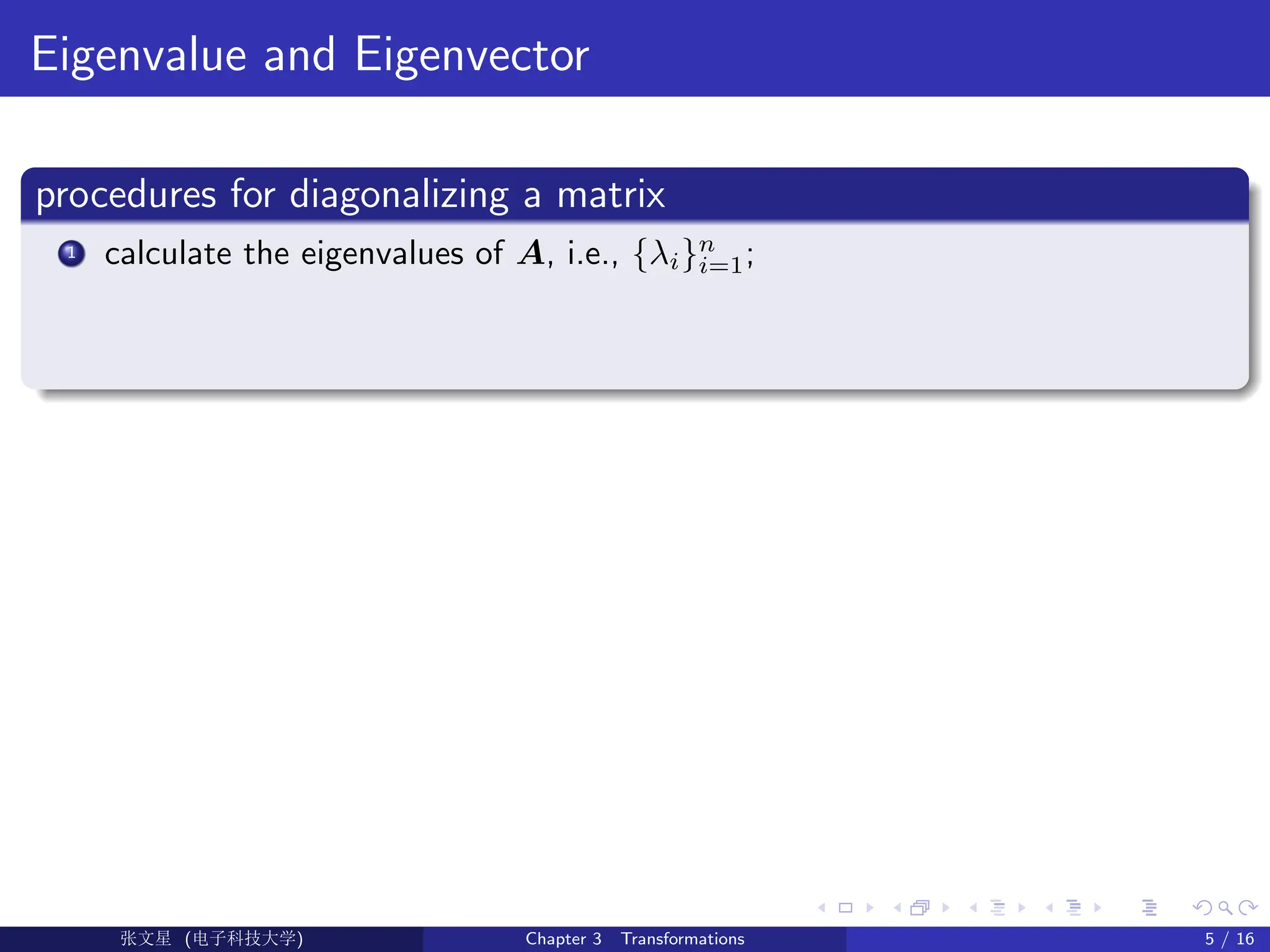
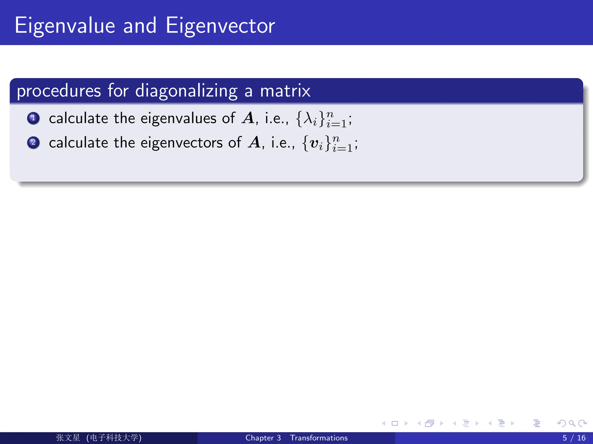
procedures for diagonalizing a matrix
1 calculate the eigenvalues of A, i.e., {λi}n
i=1;
2 calculate the eigenvectors of A, i.e., {vi}n
i=1;
3 let T = [v1, v2, . . . , vn], Λ = diag(λ1, λ2, . . . , λn), then A = T ΛT −1
.
Ü©( (>f‰EŒÆ) Chapter 3 Transformations 5 / 16](https://image.slidesharecdn.com/chapter3-251114130840-87080d8d/75/Introduction-to-Optimization-methods-lecture-1-23-2048.jpg)
![Eigenvalue and Eigenvector
procedures for diagonalizing a matrix
1 calculate the eigenvalues of A, i.e., {λi}n
i=1;
2 calculate the eigenvectors of A, i.e., {vi}n
i=1;
3 let T = [v1, v2, . . . , vn], Λ = diag(λ1, λ2, . . . , λn), then A = T ΛT −1
.
Theorem (symmetric matrix: A ∈ Rn×n
satisfying A = A>
)
Ü©( (>f‰EŒÆ) Chapter 3 Transformations 5 / 16](https://image.slidesharecdn.com/chapter3-251114130840-87080d8d/75/Introduction-to-Optimization-methods-lecture-1-24-2048.jpg)
![Eigenvalue and Eigenvector
procedures for diagonalizing a matrix
1 calculate the eigenvalues of A, i.e., {λi}n
i=1;
2 calculate the eigenvectors of A, i.e., {vi}n
i=1;
3 let T = [v1, v2, . . . , vn], Λ = diag(λ1, λ2, . . . , λn), then A = T ΛT −1
.
Theorem (symmetric matrix: A ∈ Rn×n
satisfying A = A>
)
All eigenvalues of a real symmetric matrix A ∈ Rn×n
are real.
Ü©( (>f‰EŒÆ) Chapter 3 Transformations 5 / 16](https://image.slidesharecdn.com/chapter3-251114130840-87080d8d/75/Introduction-to-Optimization-methods-lecture-1-25-2048.jpg)
![Eigenvalue and Eigenvector
procedures for diagonalizing a matrix
1 calculate the eigenvalues of A, i.e., {λi}n
i=1;
2 calculate the eigenvectors of A, i.e., {vi}n
i=1;
3 let T = [v1, v2, . . . , vn], Λ = diag(λ1, λ2, . . . , λn), then A = T ΛT −1
.
Theorem (symmetric matrix: A ∈ Rn×n
satisfying A = A>
)
All eigenvalues of a real symmetric matrix A ∈ Rn×n
are real.
Any real symmetric matrix A ∈ Rn×n
has a n mutually orthogonal
eigenvectors. (proof on blackboard)
Ü©( (>f‰EŒÆ) Chapter 3 Transformations 5 / 16](https://image.slidesharecdn.com/chapter3-251114130840-87080d8d/75/Introduction-to-Optimization-methods-lecture-1-26-2048.jpg)
![Eigenvalue and Eigenvector
procedures for diagonalizing a matrix
1 calculate the eigenvalues of A, i.e., {λi}n
i=1;
2 calculate the eigenvectors of A, i.e., {vi}n
i=1;
3 let T = [v1, v2, . . . , vn], Λ = diag(λ1, λ2, . . . , λn), then A = T ΛT −1
.
Theorem (symmetric matrix: A ∈ Rn×n
satisfying A = A>
)
All eigenvalues of a real symmetric matrix A ∈ Rn×n
are real.
Any real symmetric matrix A ∈ Rn×n
has a n mutually orthogonal
eigenvectors. (proof on blackboard)
Definition (orthogonal matrix)
A matrix whose transpose is its inverse is said to be an orthogonal matrix, i.e.,
T −1
= T >
.
Ü©( (>f‰EŒÆ) Chapter 3 Transformations 5 / 16](https://image.slidesharecdn.com/chapter3-251114130840-87080d8d/75/Introduction-to-Optimization-methods-lecture-1-27-2048.jpg)
![Eigenvalue and Eigenvector
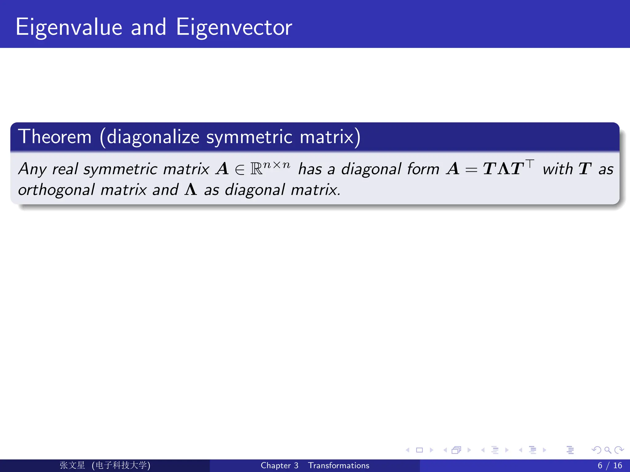
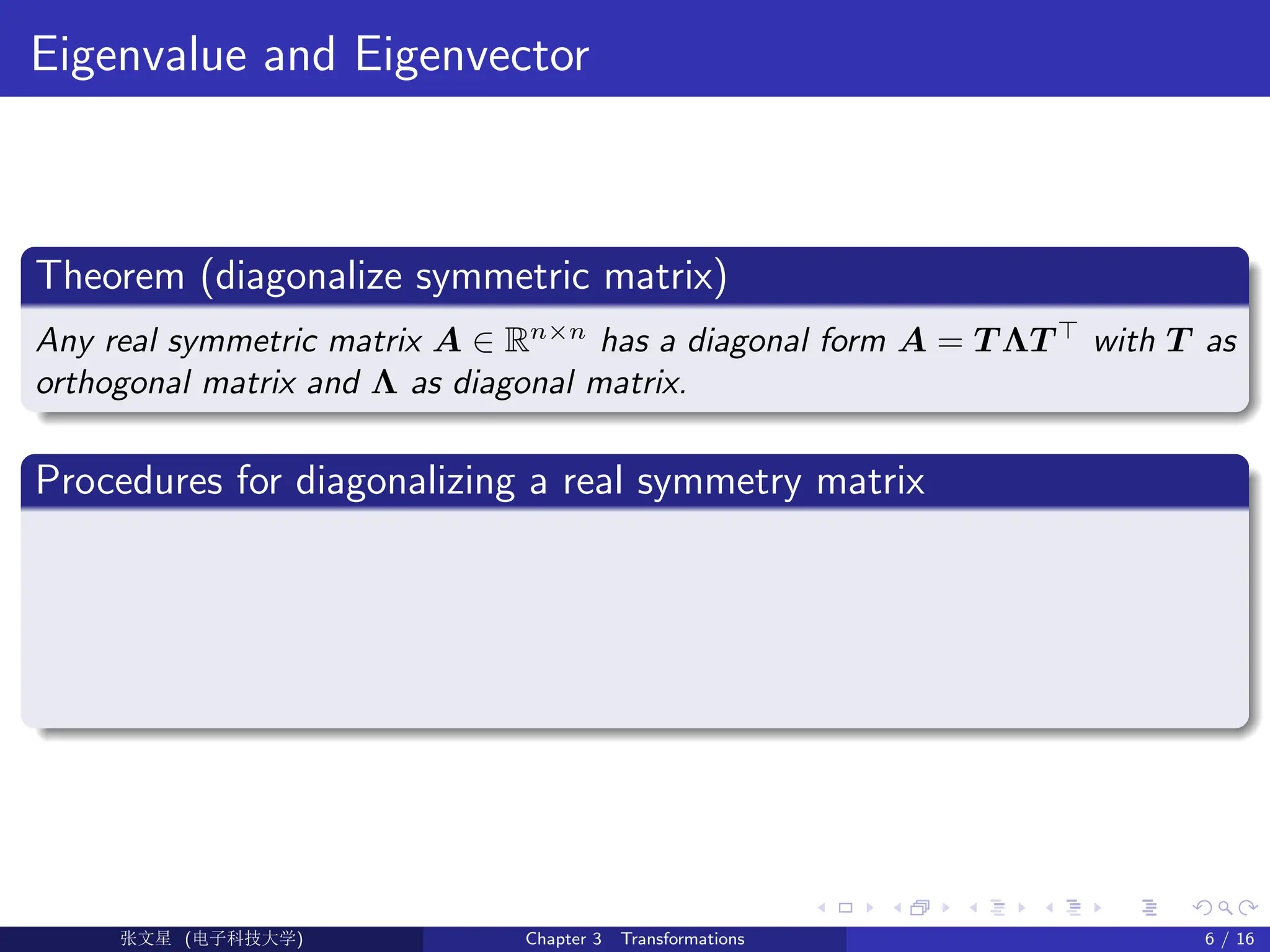
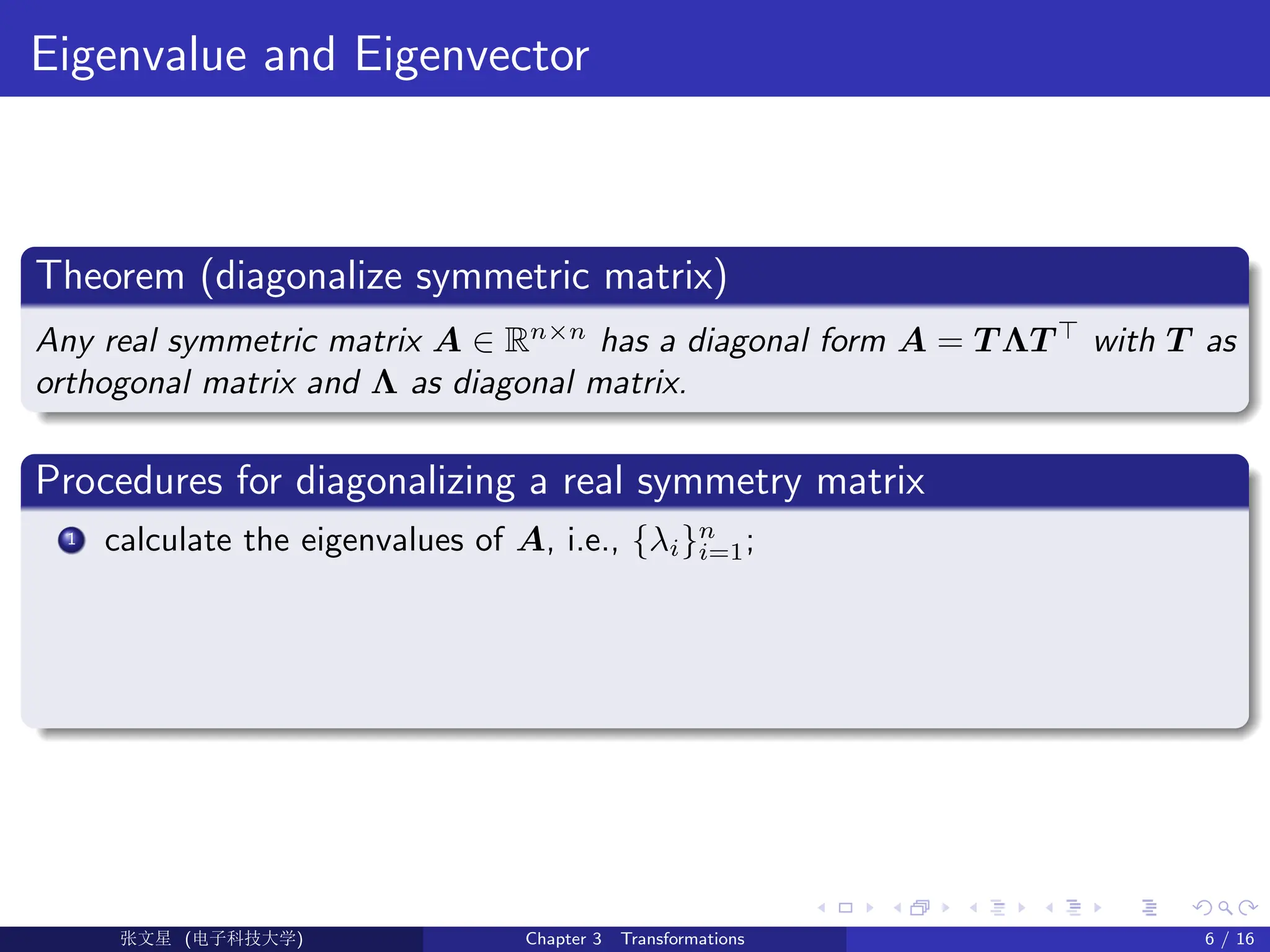
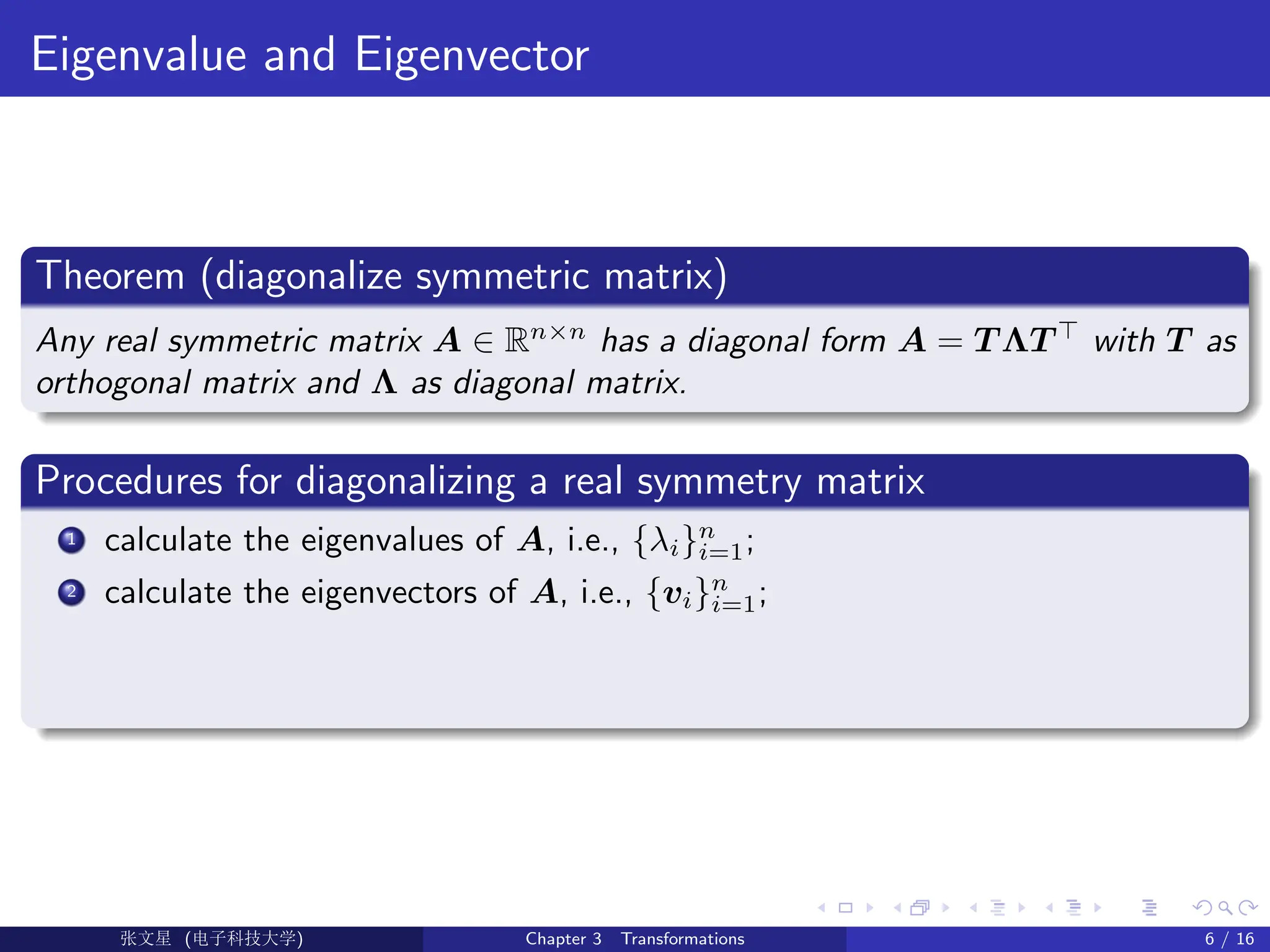
Theorem (diagonalize symmetric matrix)
Any real symmetric matrix A ∈ Rn×n
has a diagonal form A = T ΛT >
with T as
orthogonal matrix and Λ as diagonal matrix.
Procedures for diagonalizing a real symmetry matrix
1 calculate the eigenvalues of A, i.e., {λi}n
i=1;
2 calculate the eigenvectors of A, i.e., {vi}n
i=1;
3 normalize individually the eigenvectors of λi, T = [u1, u2, . . . , un]
Ü©( (>f‰EŒÆ) Chapter 3 Transformations 6 / 16](https://image.slidesharecdn.com/chapter3-251114130840-87080d8d/75/Introduction-to-Optimization-methods-lecture-1-32-2048.jpg)
![Eigenvalue and Eigenvector
Theorem (diagonalize symmetric matrix)
Any real symmetric matrix A ∈ Rn×n
has a diagonal form A = T ΛT >
with T as
orthogonal matrix and Λ as diagonal matrix.
Procedures for diagonalizing a real symmetry matrix
1 calculate the eigenvalues of A, i.e., {λi}n
i=1;
2 calculate the eigenvectors of A, i.e., {vi}n
i=1;
3 normalize individually the eigenvectors of λi, T = [u1, u2, . . . , un]
4 let T = [u1, . . . , un], Λ = diag(λ1, . . . , λn), then A = T ΛT −1
= T ΛT >
.
Ü©( (>f‰EŒÆ) Chapter 3 Transformations 6 / 16](https://image.slidesharecdn.com/chapter3-251114130840-87080d8d/75/Introduction-to-Optimization-methods-lecture-1-33-2048.jpg)
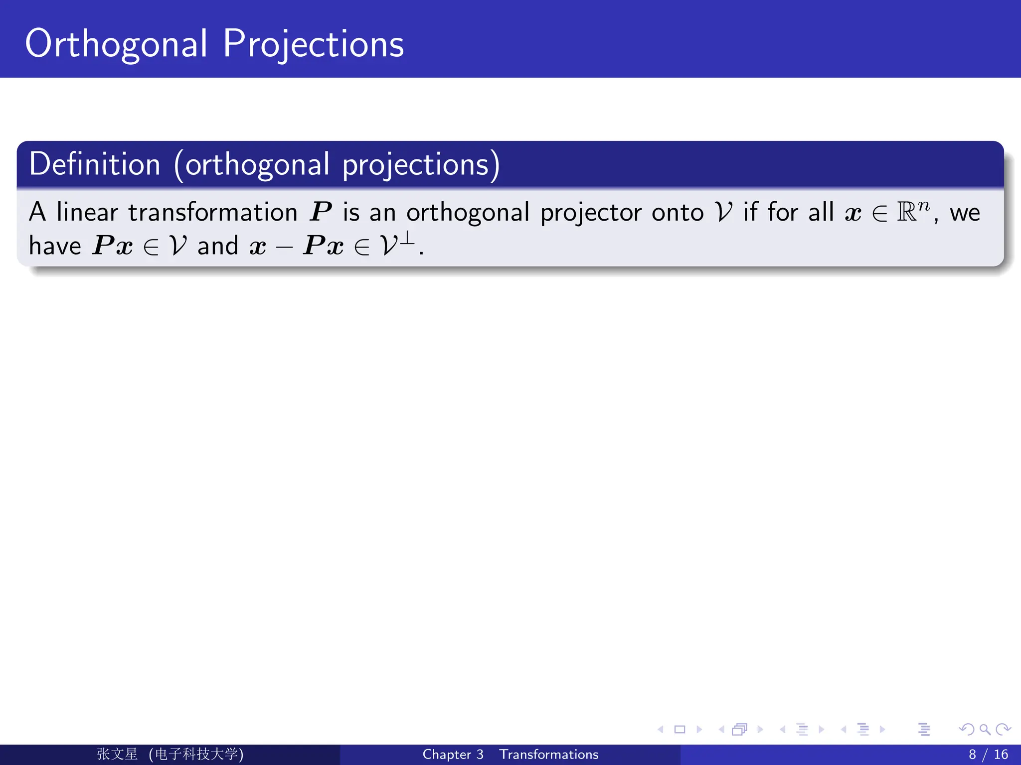
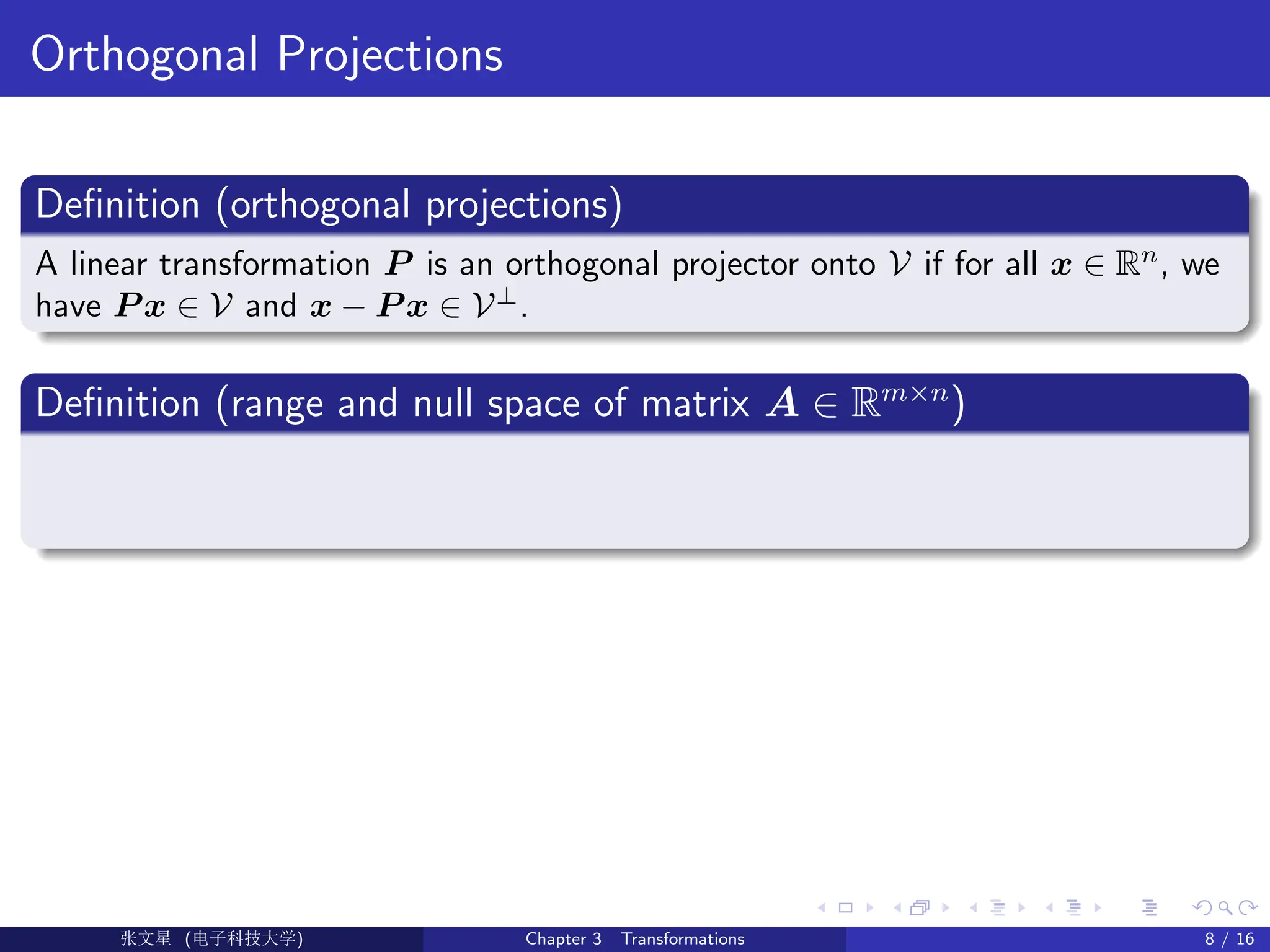
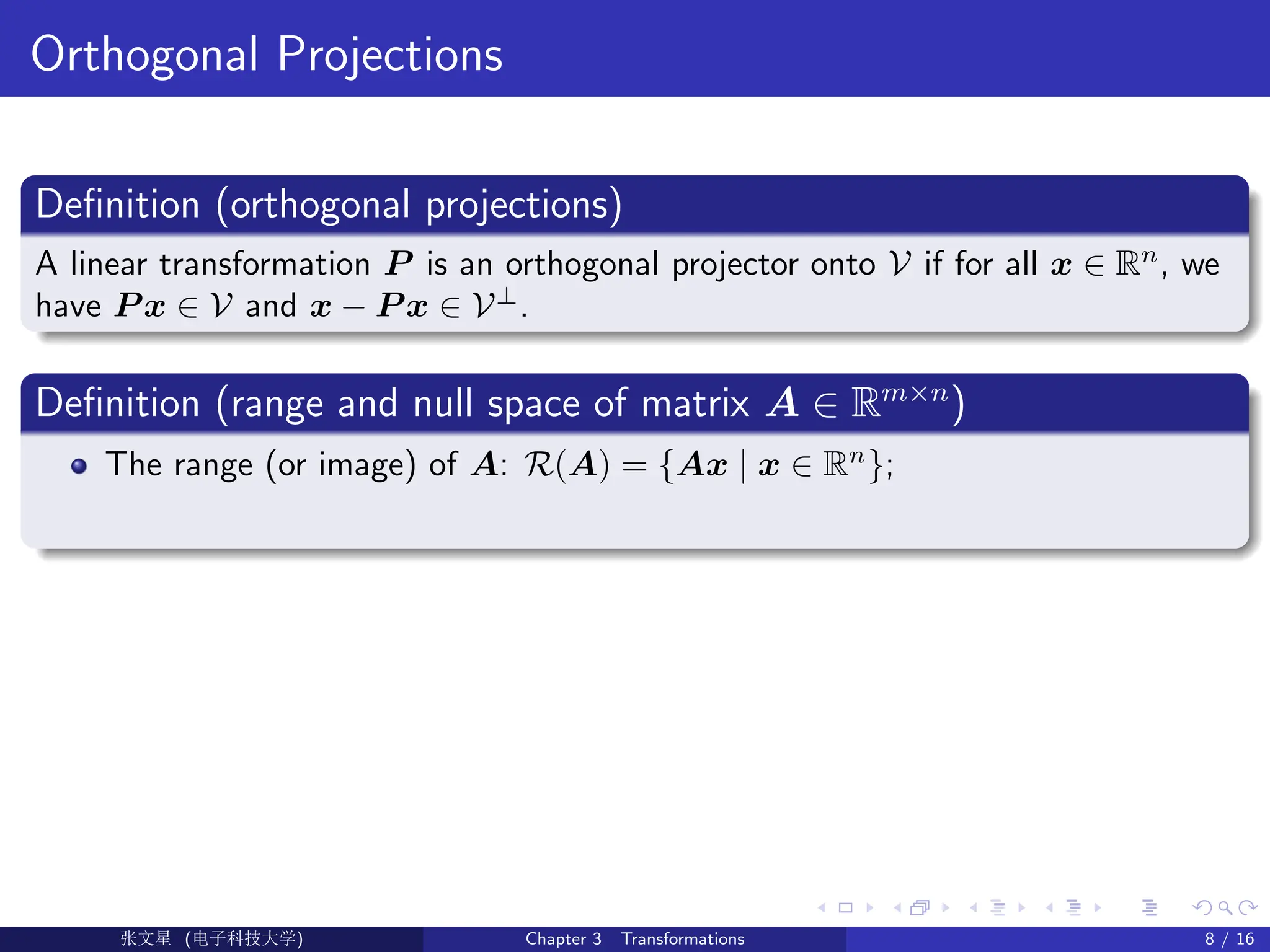
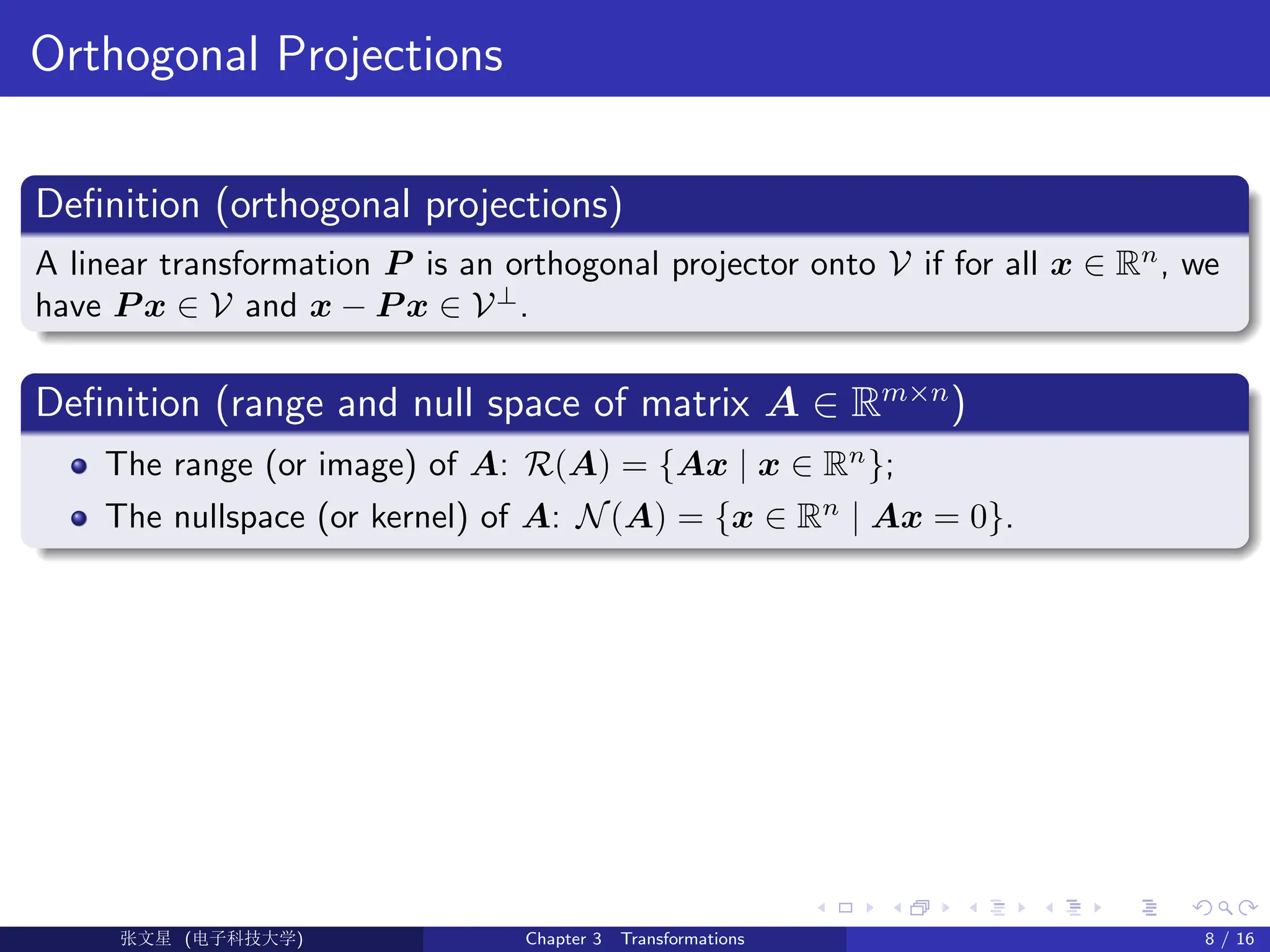
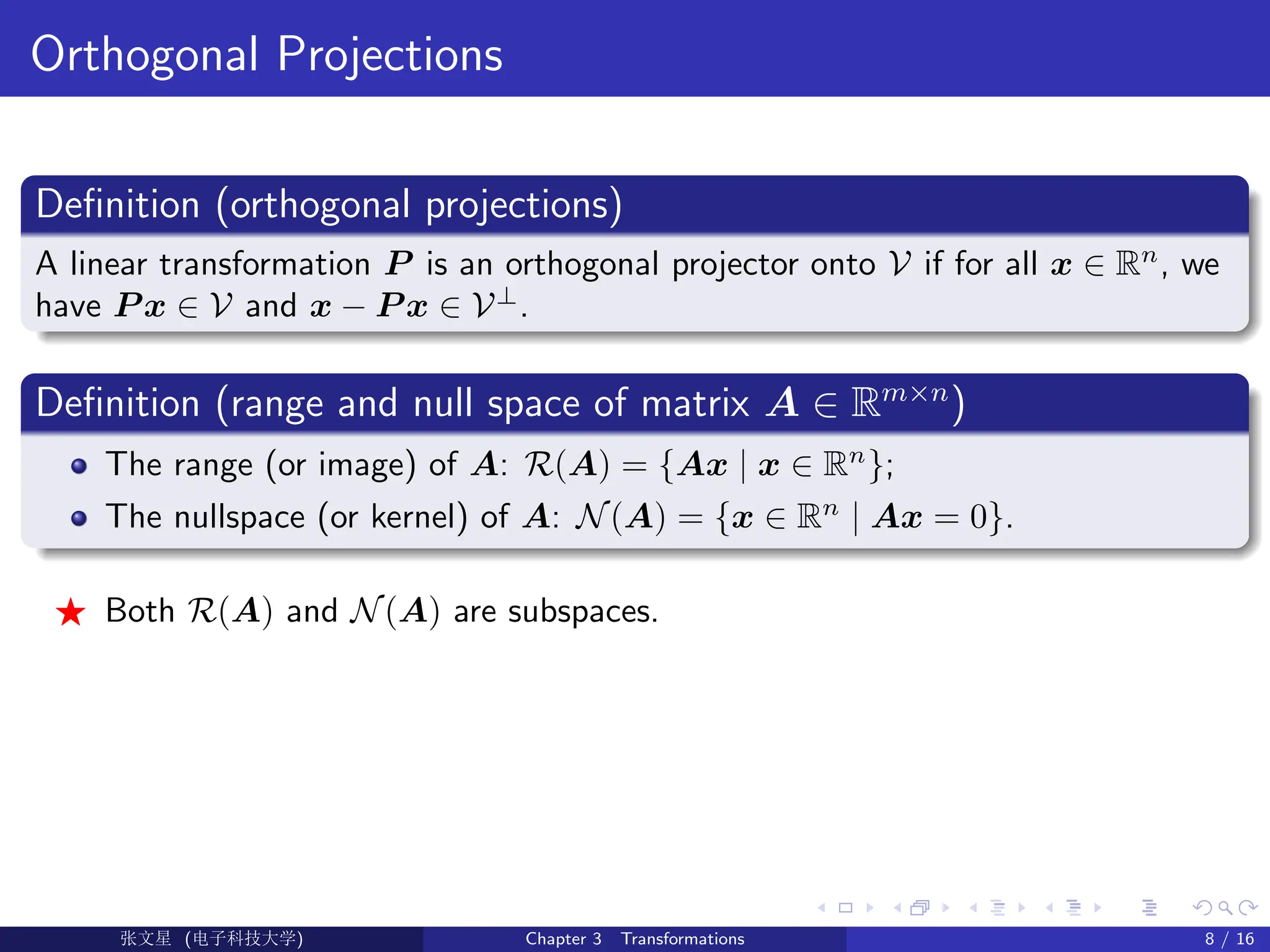
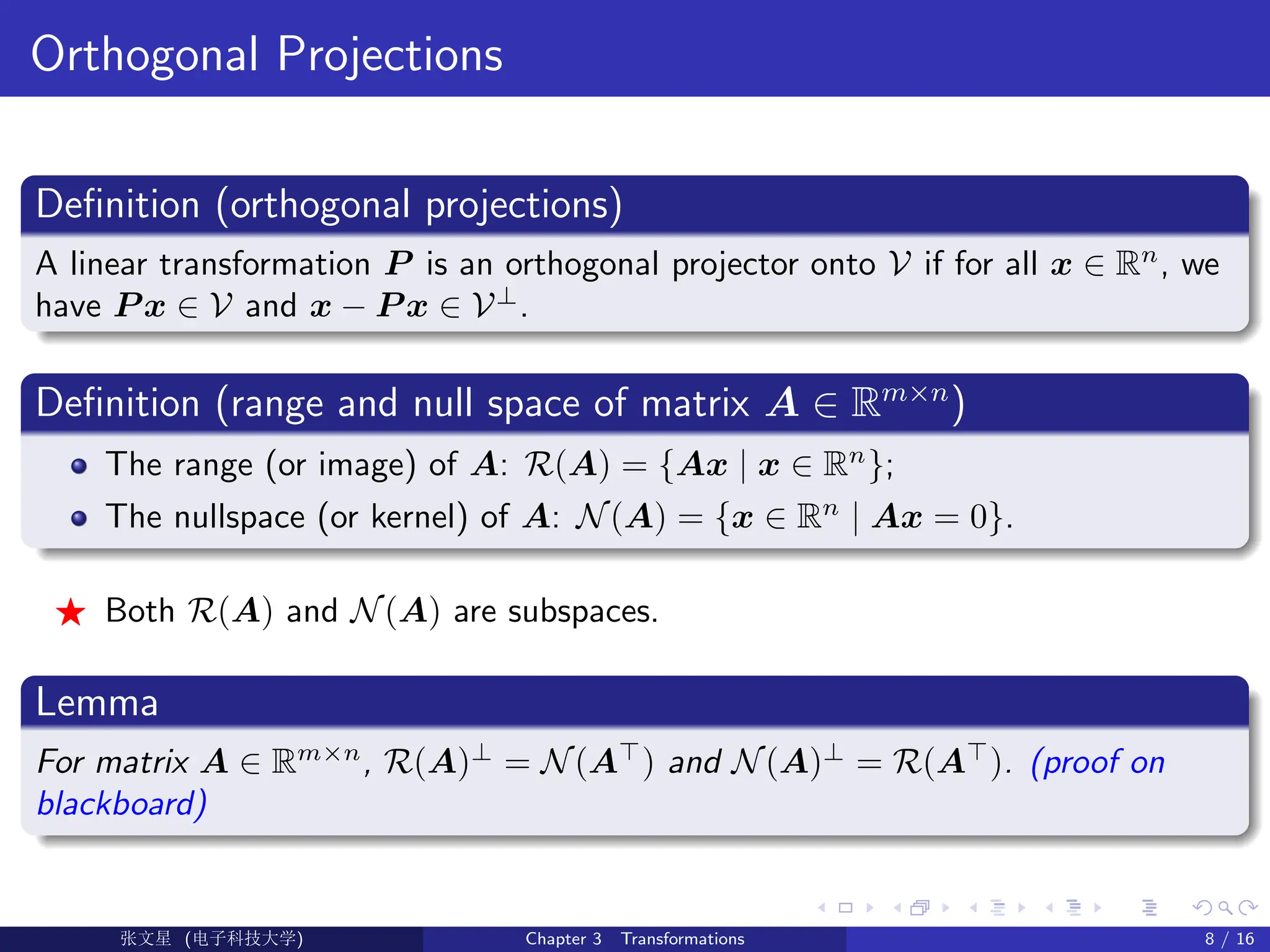
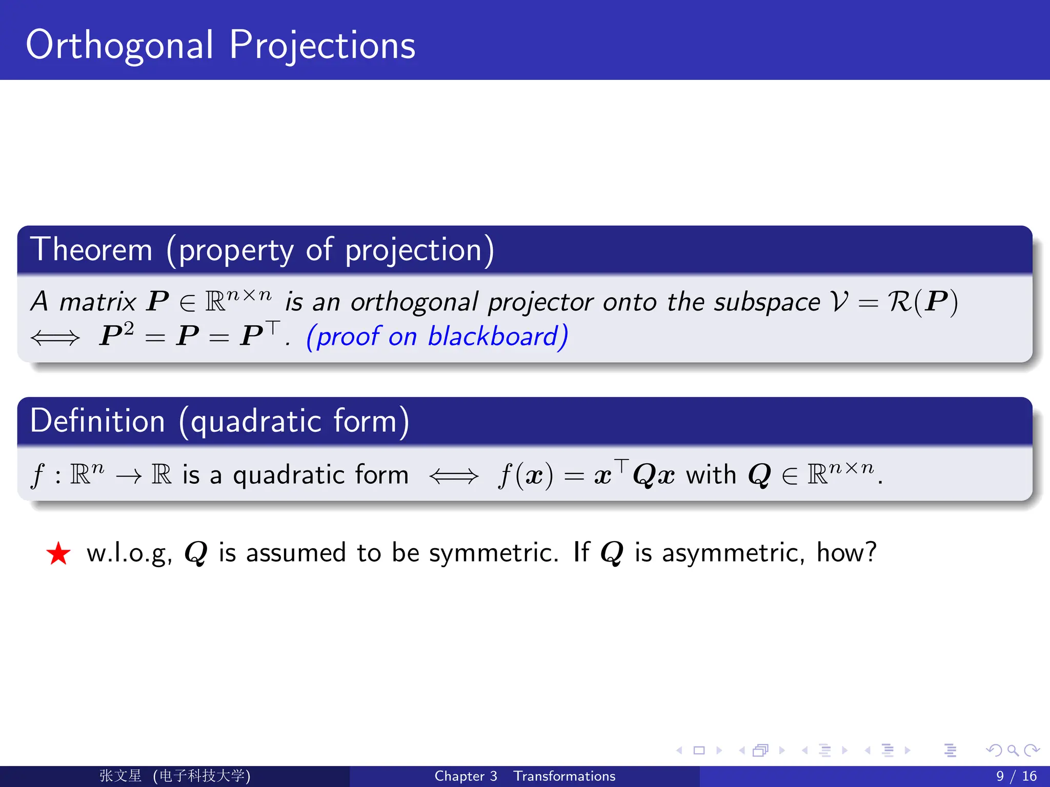
![Orthogonal Projections
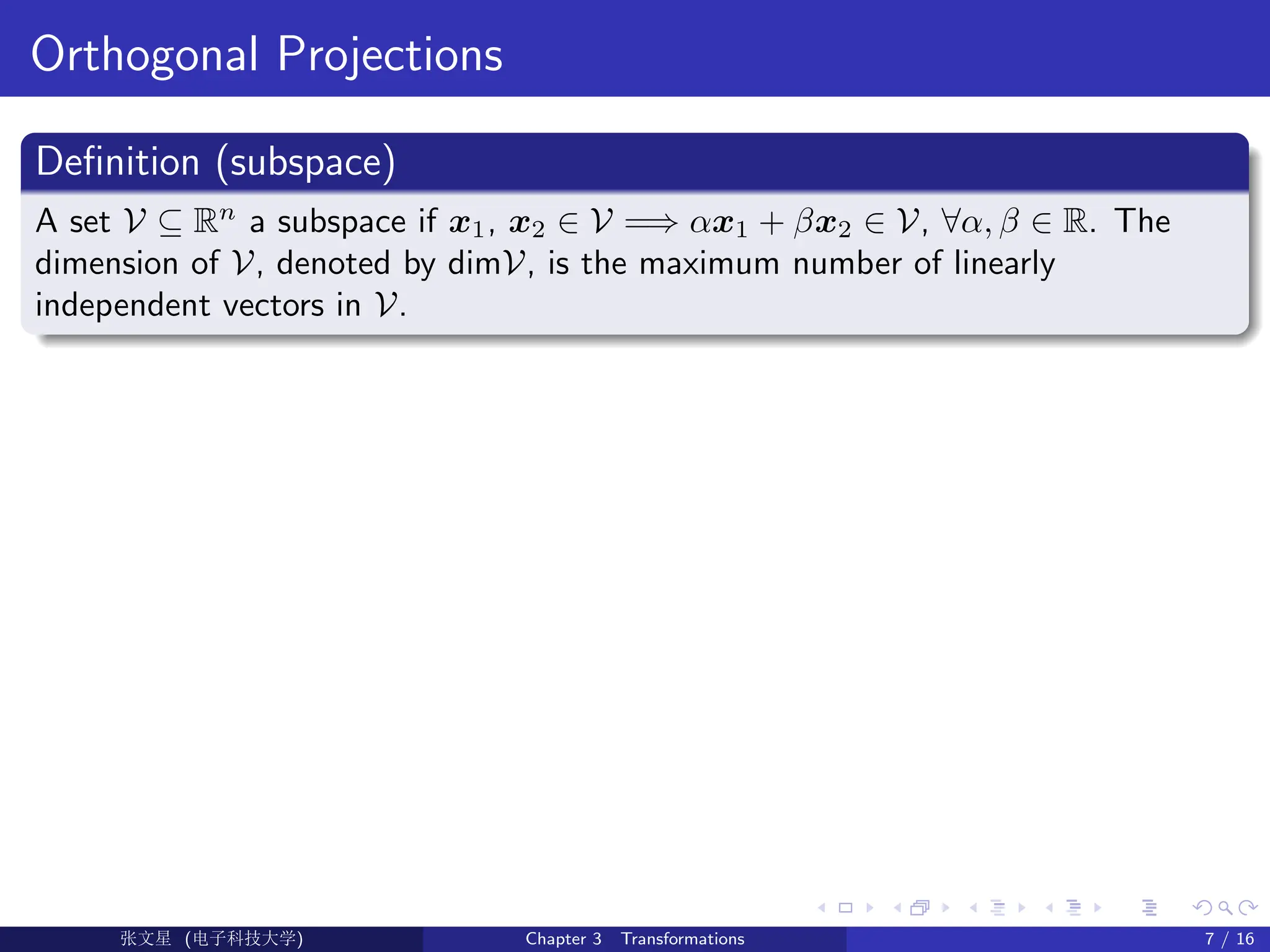
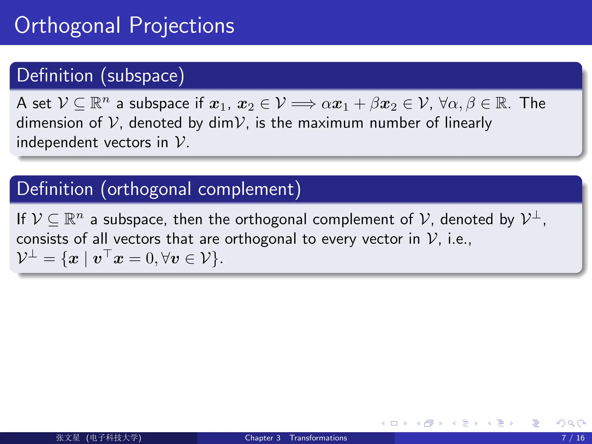
Definition (subspace)
A set V ⊆ Rn
a subspace if x1, x2 ∈ V =⇒ αx1 + βx2 ∈ V, ∀α, β ∈ R. The
dimension of V, denoted by dimV, is the maximum number of linearly
independent vectors in V.
Definition (orthogonal complement)
If V ⊆ Rn
a subspace, then the orthogonal complement of V, denoted by V⊥
,
consists of all vectors that are orthogonal to every vector in V, i.e.,
V⊥
= {x | v>
x = 0, ∀v ∈ V}.
F V ⊥
is also a subspace of Rn
. V and V⊥
span Rn
(or Rn
is the direct sum of V
and V⊥
), i.e., Rn
= V ⊕ V⊥
. Concisely, every x ∈ Rn
can be represented
uniquely as
[orthogonal decomposition] x = x1 + x2, where x1 ∈ V, x2 ∈ V⊥
.
Ü©( (>f‰EŒÆ) Chapter 3 Transformations 7 / 16](https://image.slidesharecdn.com/chapter3-251114130840-87080d8d/75/Introduction-to-Optimization-methods-lecture-1-36-2048.jpg)
![Orthogonal Projections
Definition (subspace)
A set V ⊆ Rn
a subspace if x1, x2 ∈ V =⇒ αx1 + βx2 ∈ V, ∀α, β ∈ R. The
dimension of V, denoted by dimV, is the maximum number of linearly
independent vectors in V.
Definition (orthogonal complement)
If V ⊆ Rn
a subspace, then the orthogonal complement of V, denoted by V⊥
,
consists of all vectors that are orthogonal to every vector in V, i.e.,
V⊥
= {x | v>
x = 0, ∀v ∈ V}.
F V ⊥
is also a subspace of Rn
. V and V⊥
span Rn
(or Rn
is the direct sum of V
and V⊥
), i.e., Rn
= V ⊕ V⊥
. Concisely, every x ∈ Rn
can be represented
uniquely as
[orthogonal decomposition] x = x1 + x2, where x1 ∈ V, x2 ∈ V⊥
.
F x1 (resp. x2) is orthogonal projections of x onto V (resp. V⊥
).
Ü©( (>f‰EŒÆ) Chapter 3 Transformations 7 / 16](https://image.slidesharecdn.com/chapter3-251114130840-87080d8d/75/Introduction-to-Optimization-methods-lecture-1-37-2048.jpg)
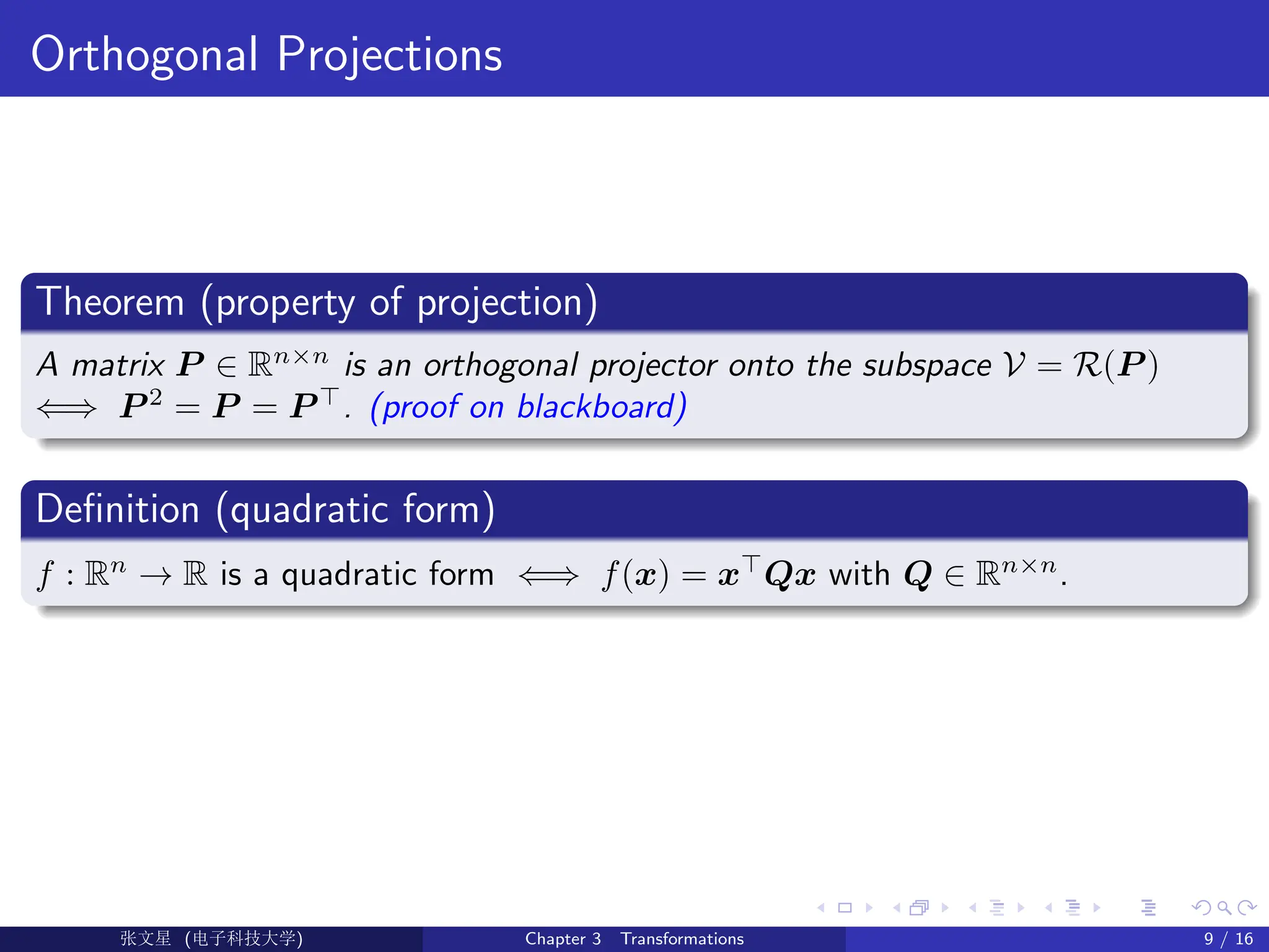
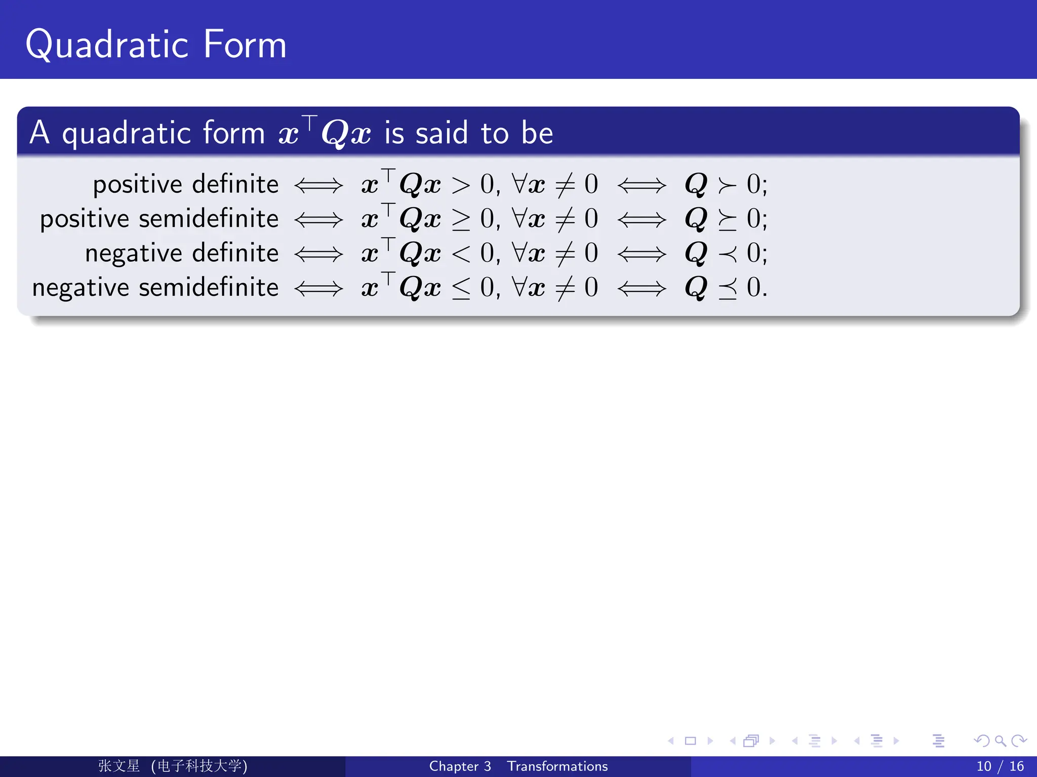
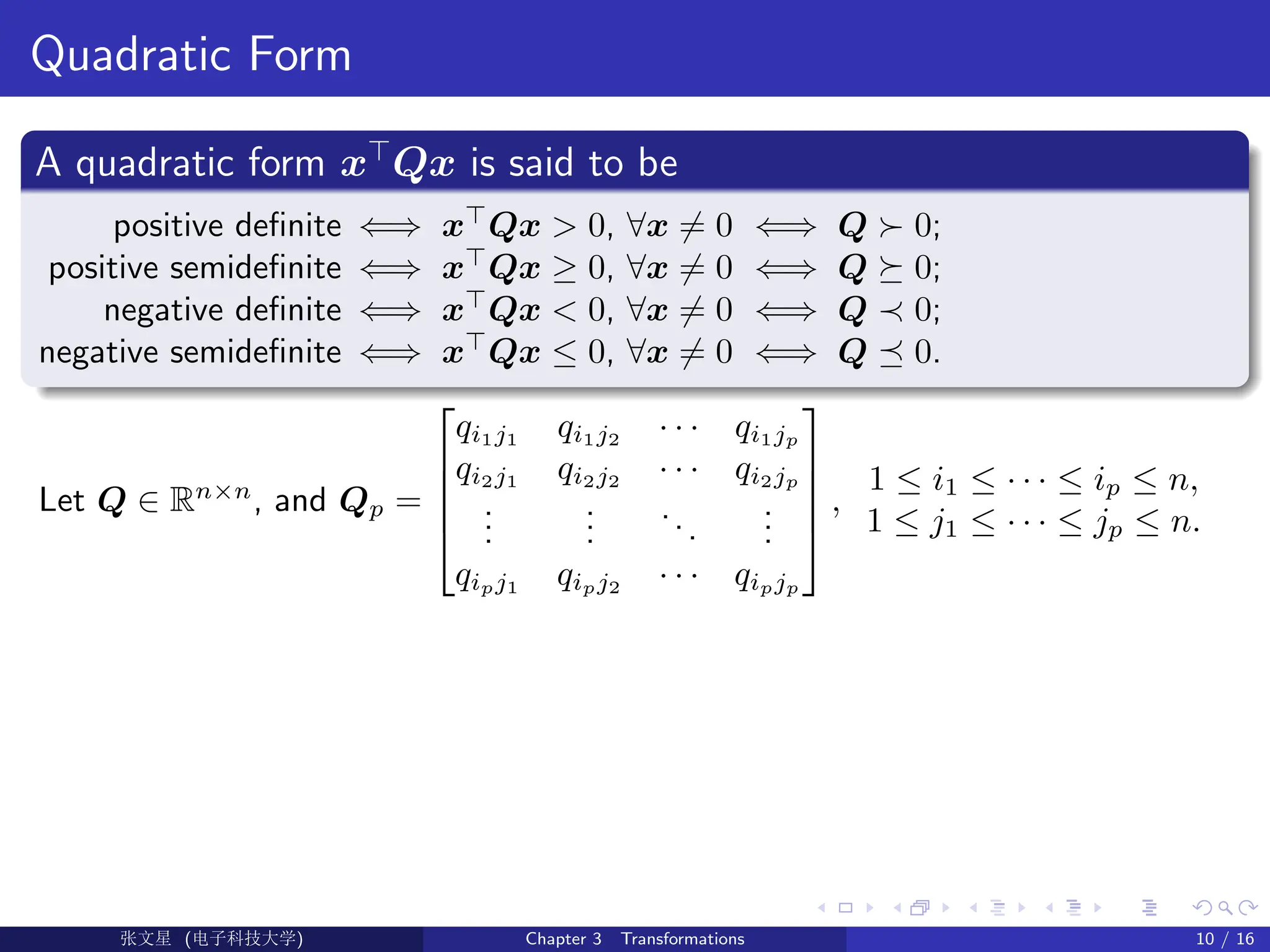
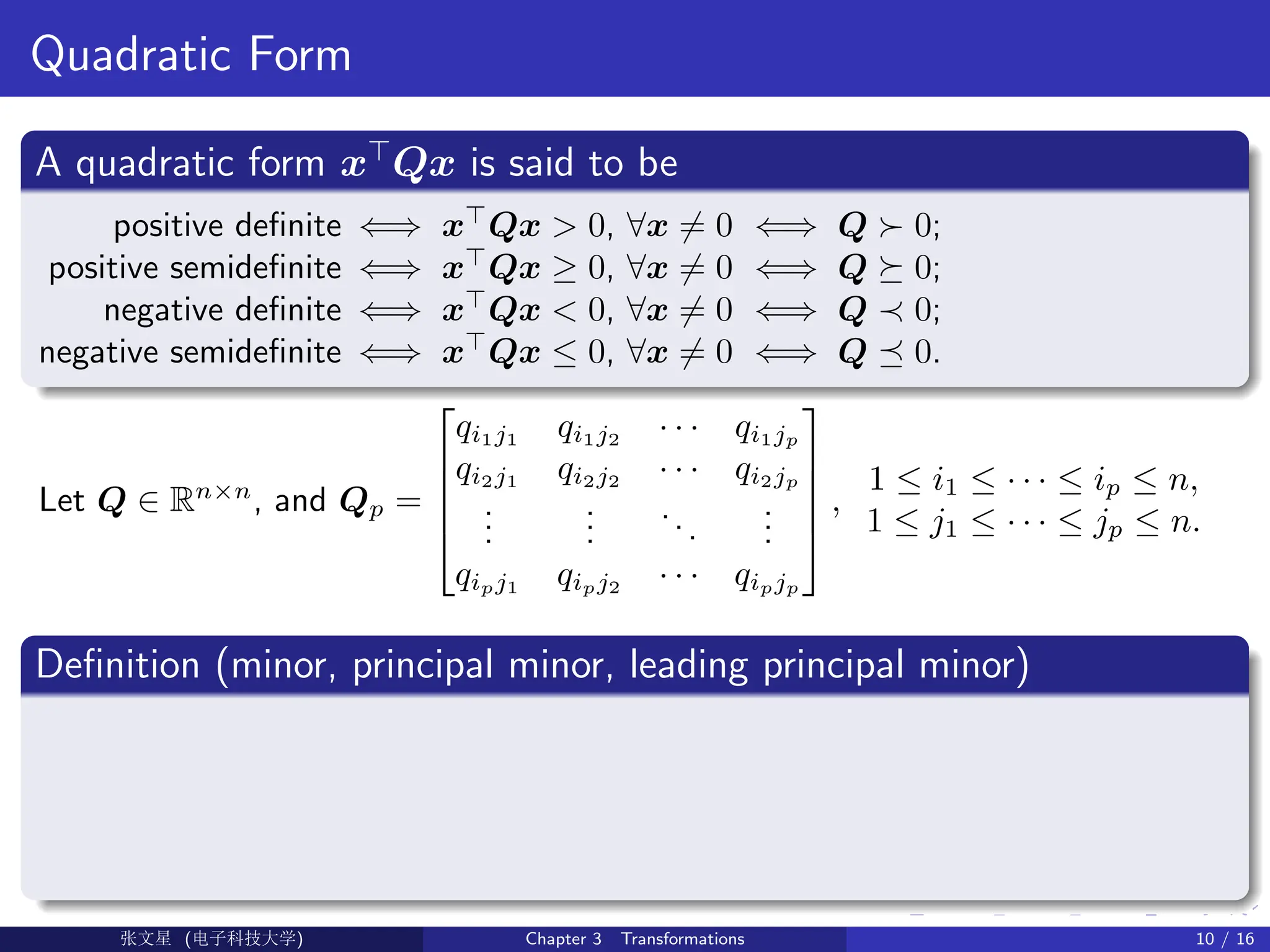
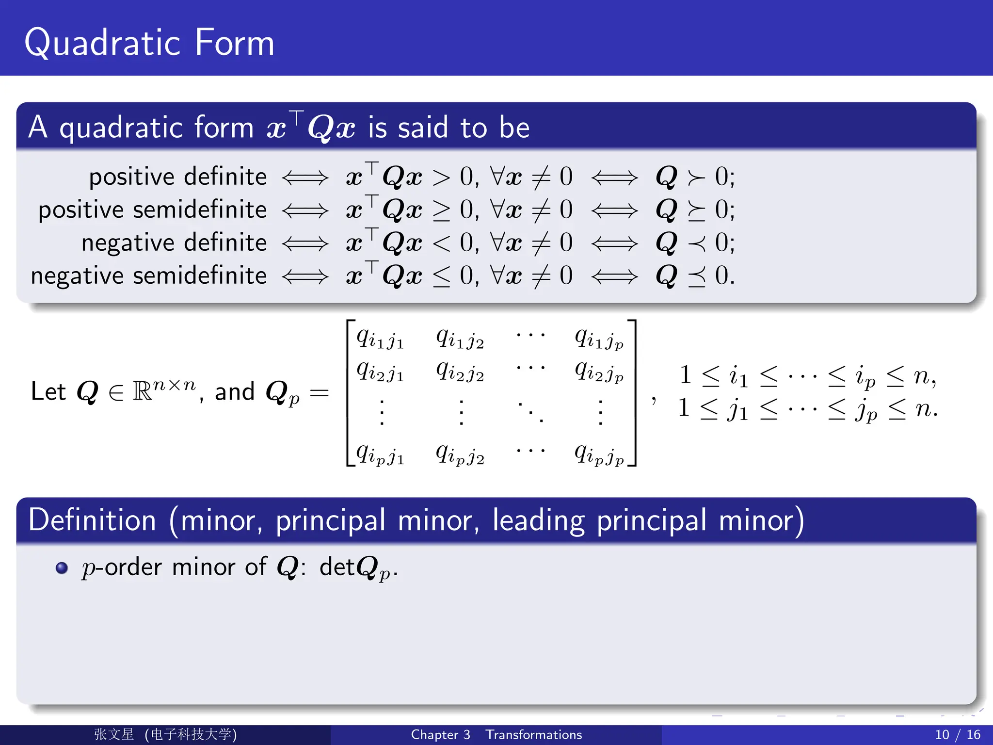
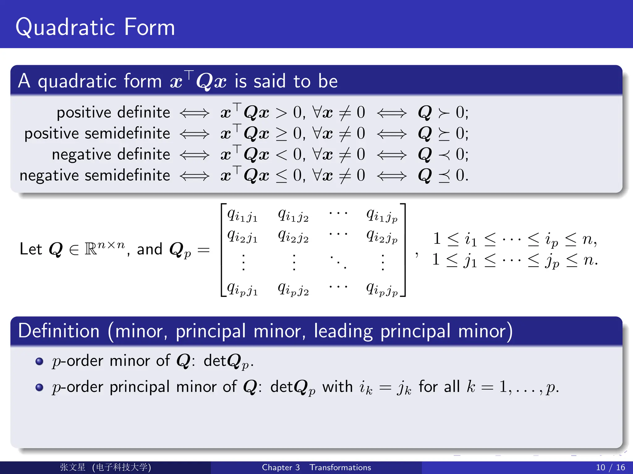
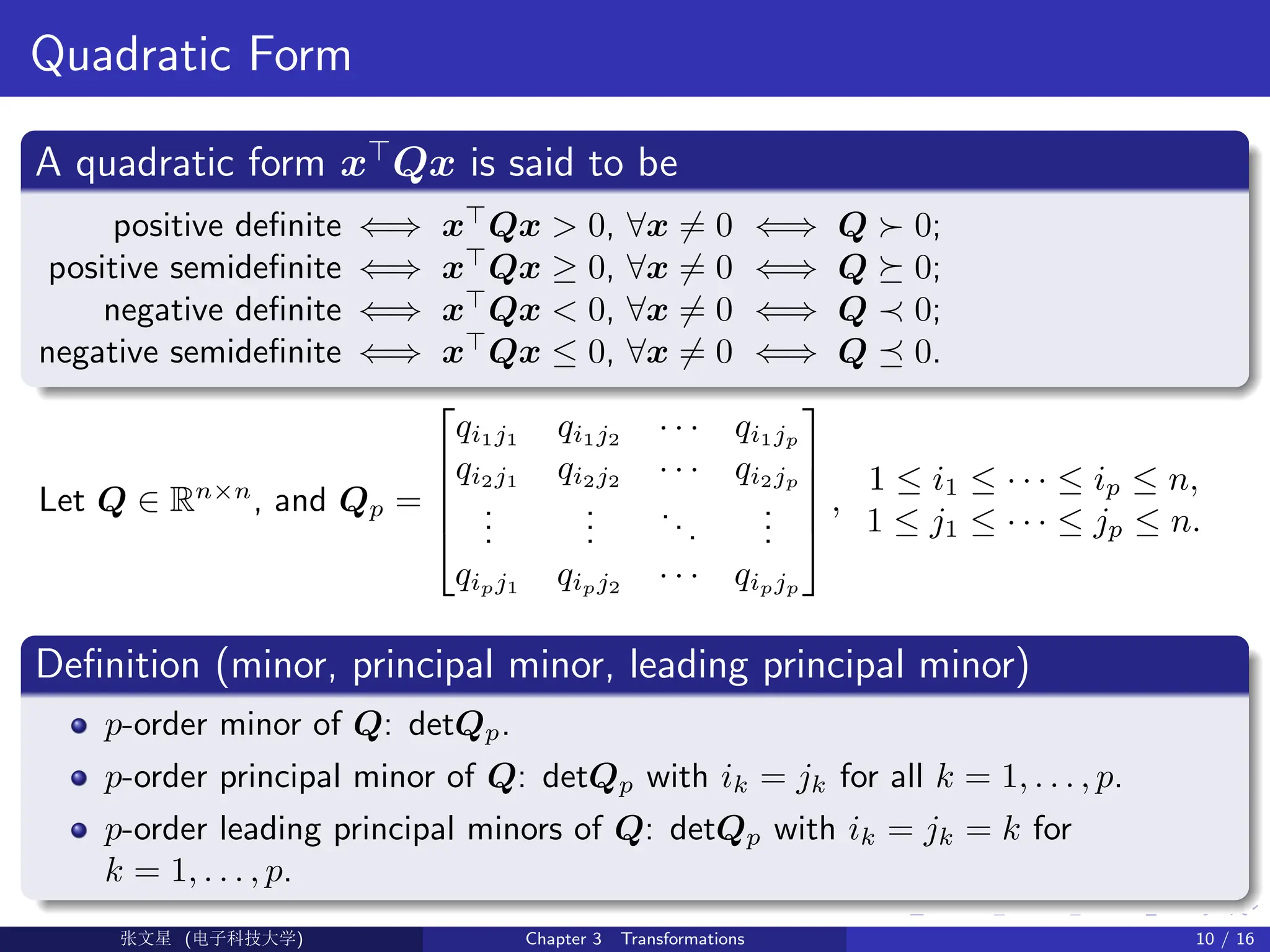

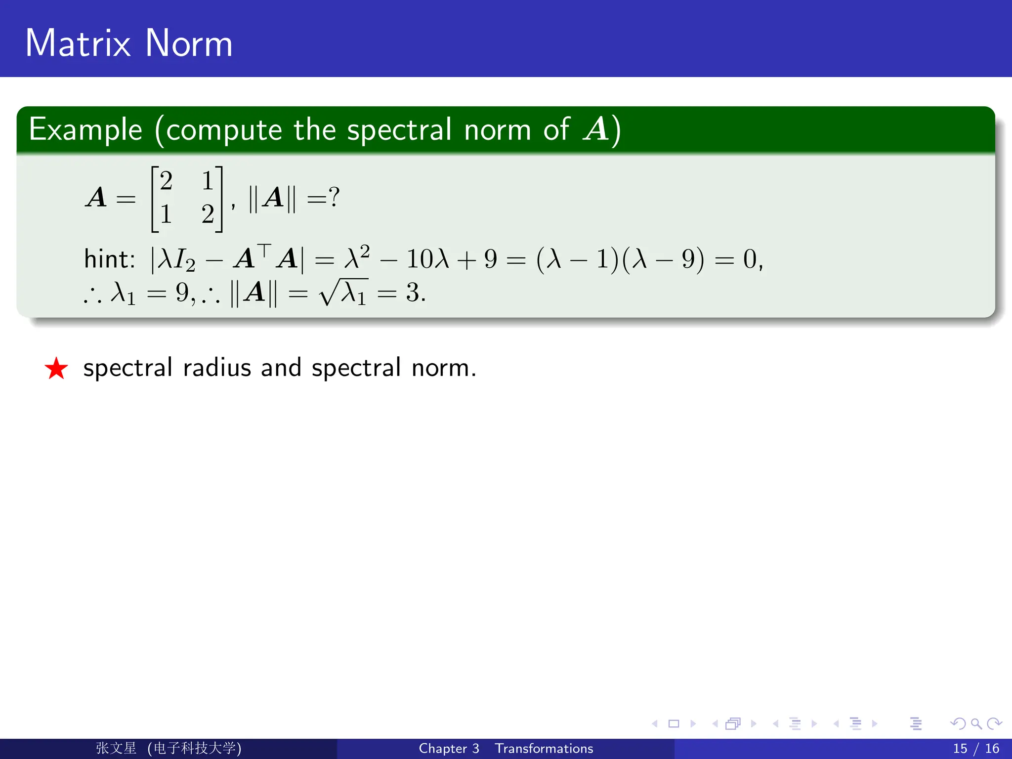
![Quadratic Form
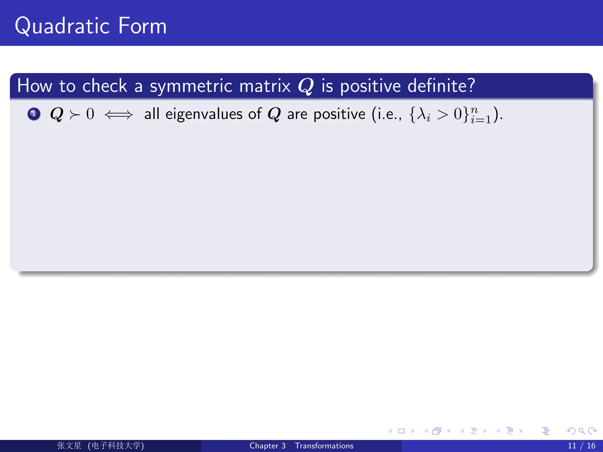
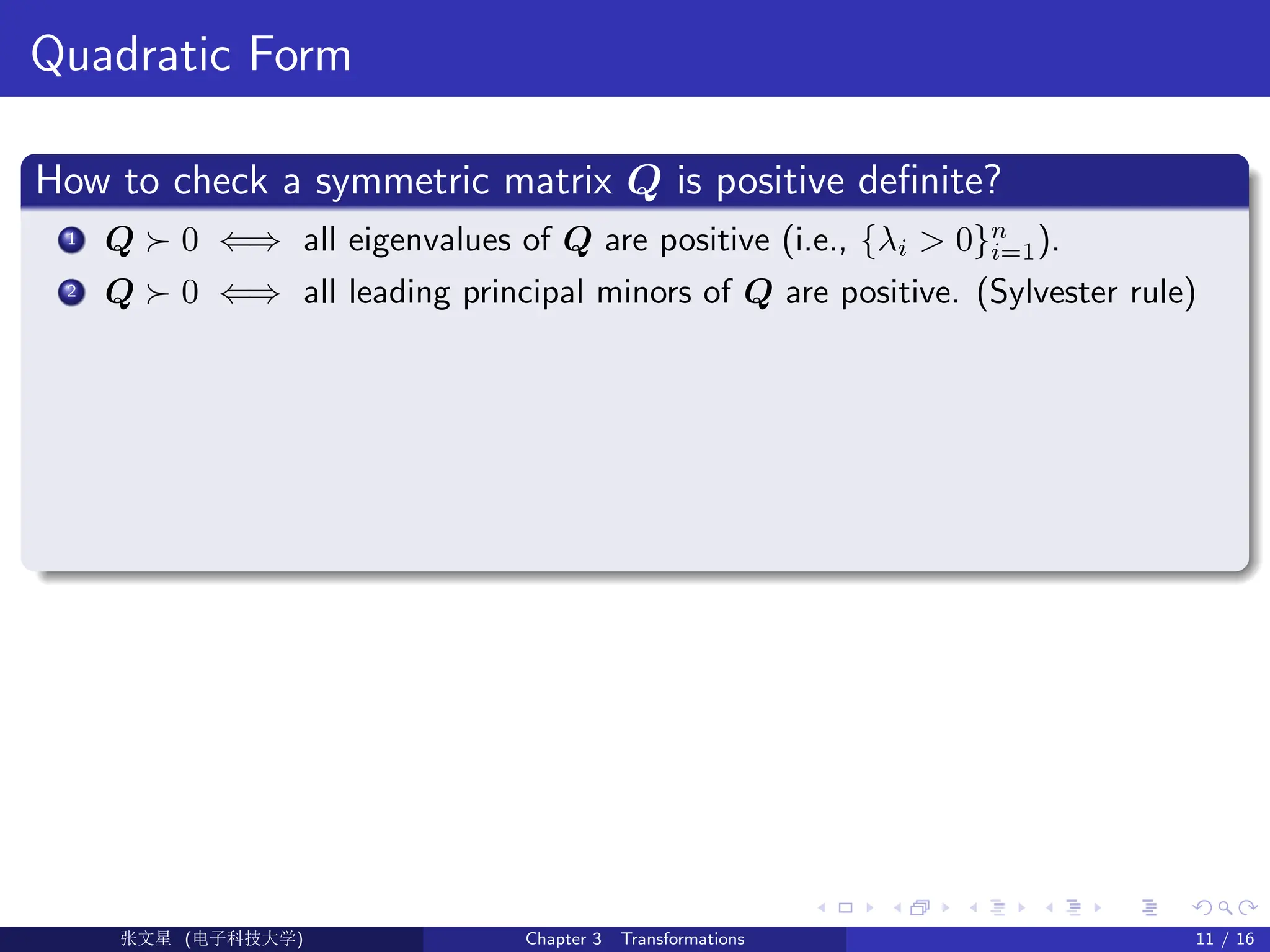
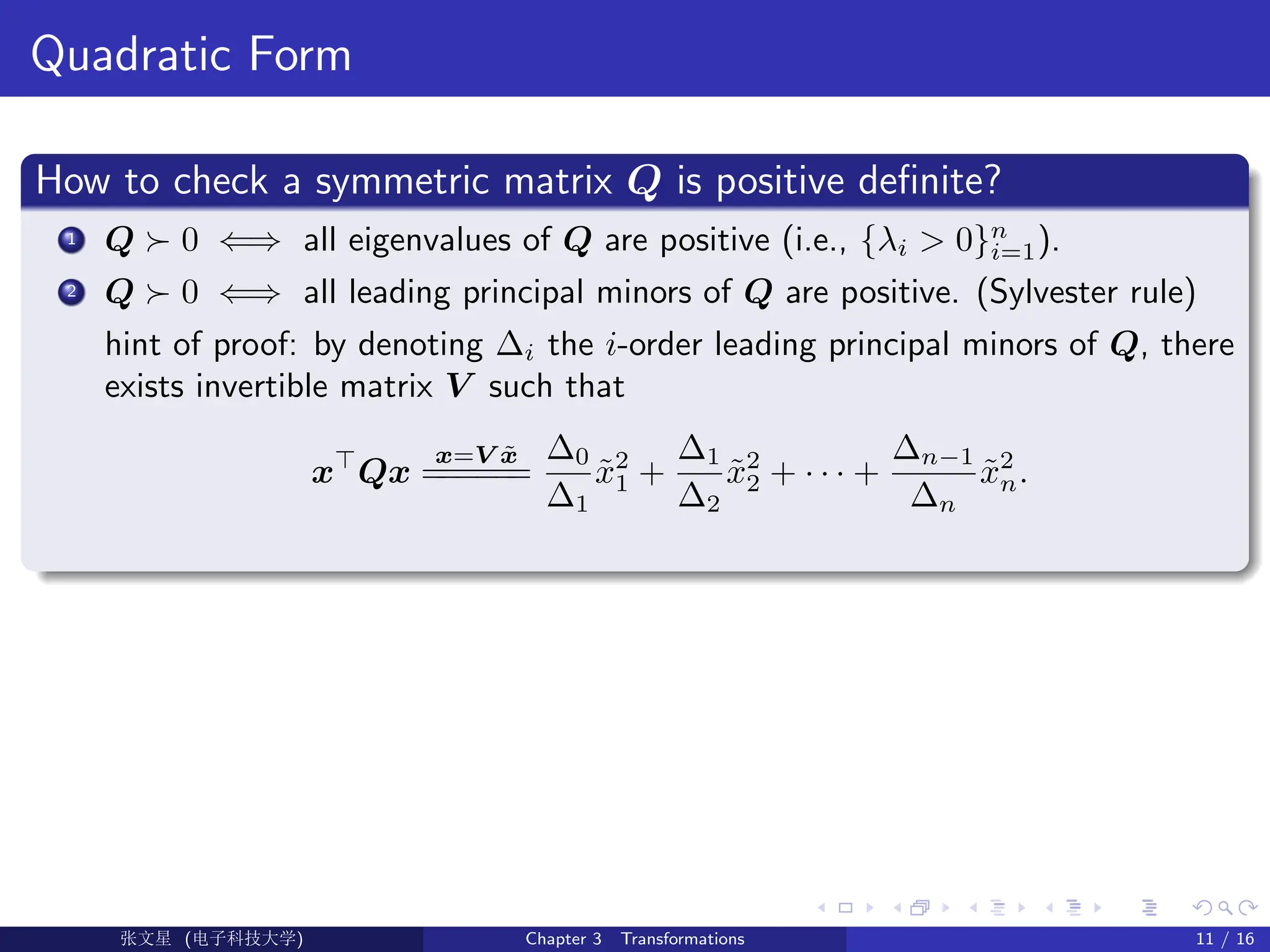
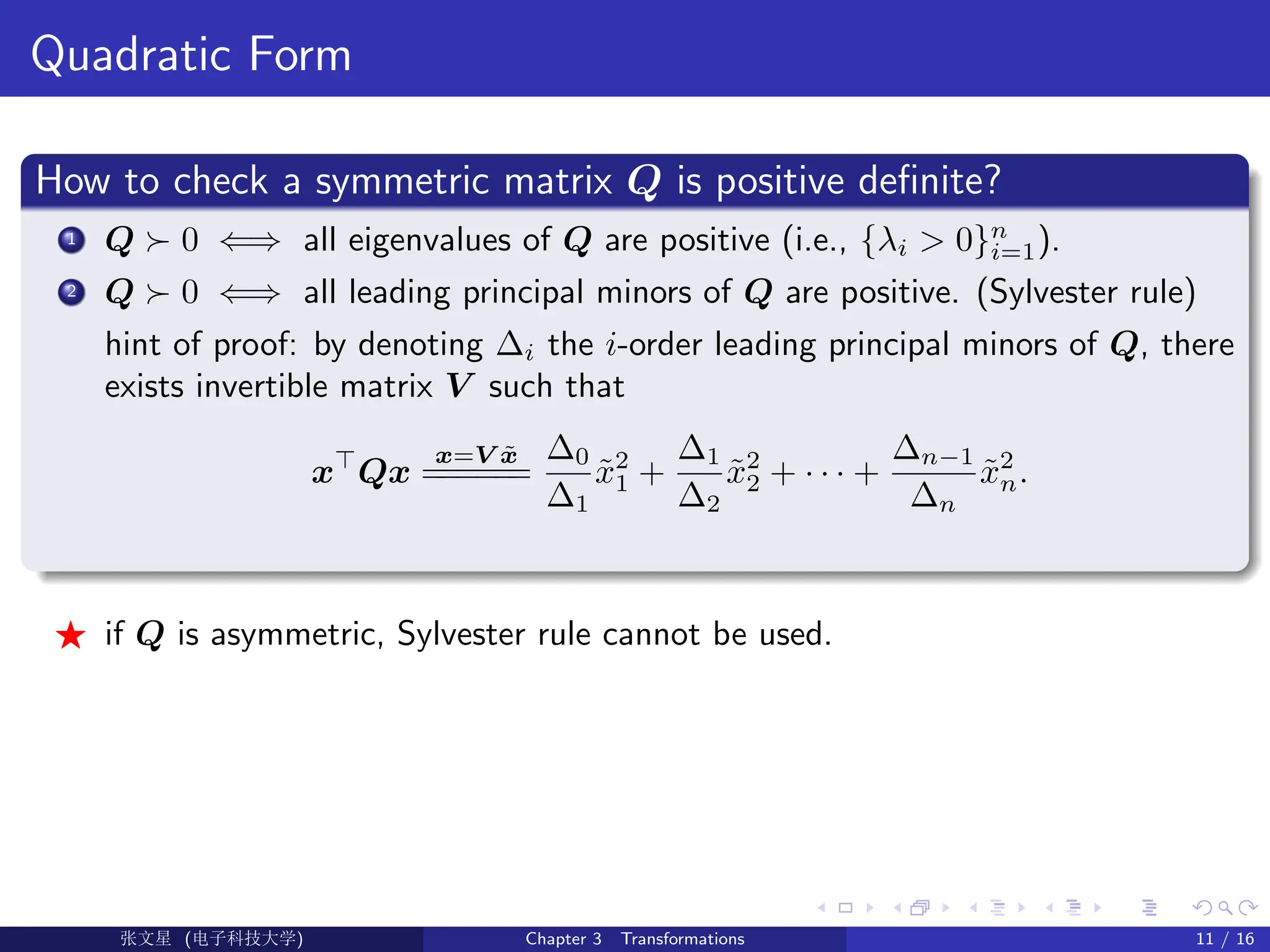
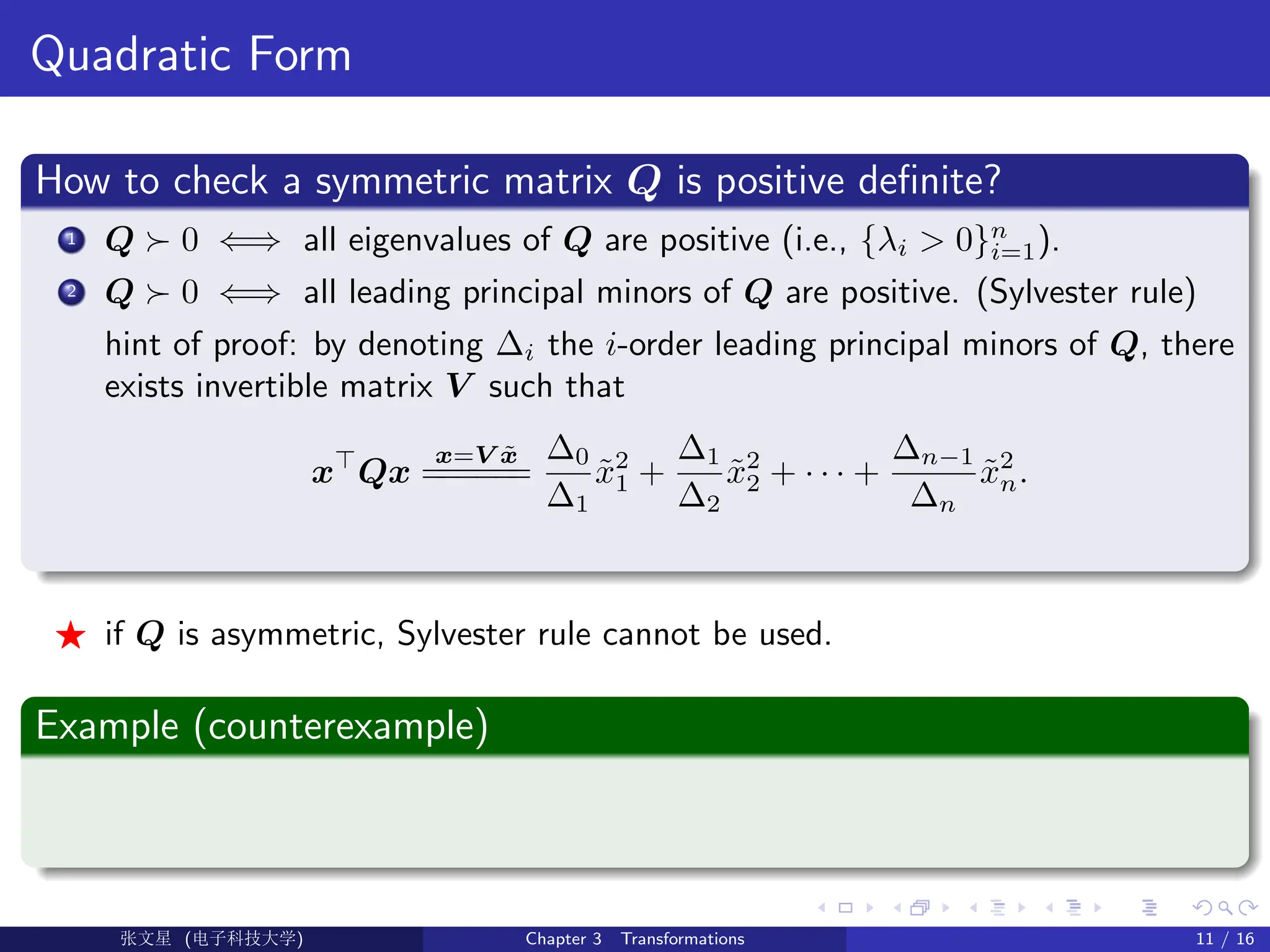
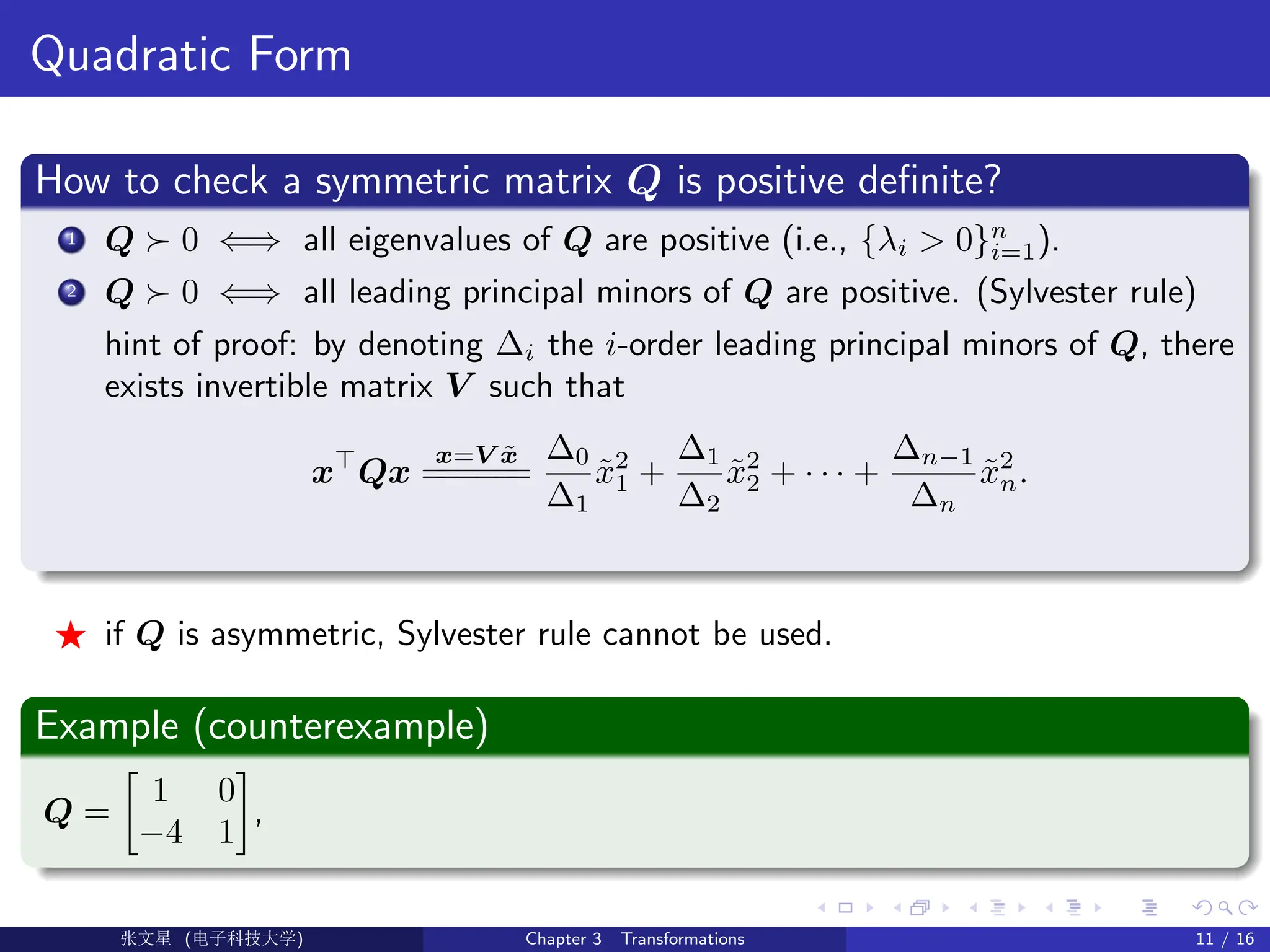
How to check a symmetric matrix Q is positive definite?
1 Q 0 ⇐⇒ all eigenvalues of Q are positive (i.e., {λi 0}n
i=1).
2 Q 0 ⇐⇒ all leading principal minors of Q are positive. (Sylvester rule)
hint of proof: by denoting ∆i the i-order leading principal minors of Q, there
exists invertible matrix V such that
x
Qx
x=V x̃
=
=
=
=
=
=
∆0
∆1
x̃2
1 +
∆1
∆2
x̃2
2 + · · · +
∆n−1
∆n
x̃2
n.
F if Q is asymmetric, Sylvester rule cannot be used.
Example (counterexample)
Q =
1 0
−4 1
,
Although ∆1 = 1 0 and ∆2 = detQ = 1 0, Q 0
(∵ x = [1, 1]
=⇒ x
Qx = −2 0).
Ü©( (f‰EŒÆ) Chapter 3 Transformations 11 / 16](https://image.slidesharecdn.com/chapter3-251114130840-87080d8d/75/Introduction-to-Optimization-methods-lecture-1-61-2048.jpg)
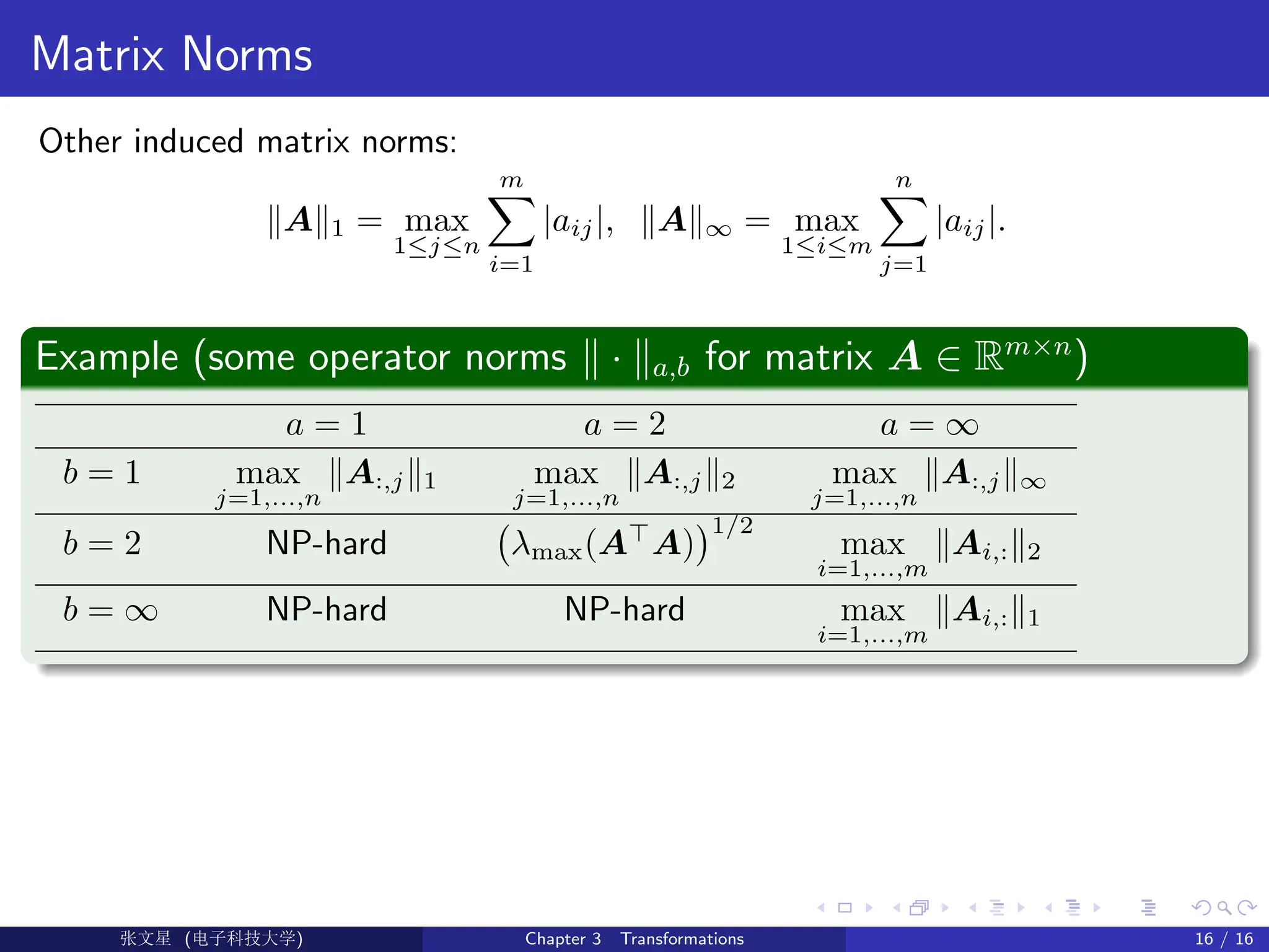
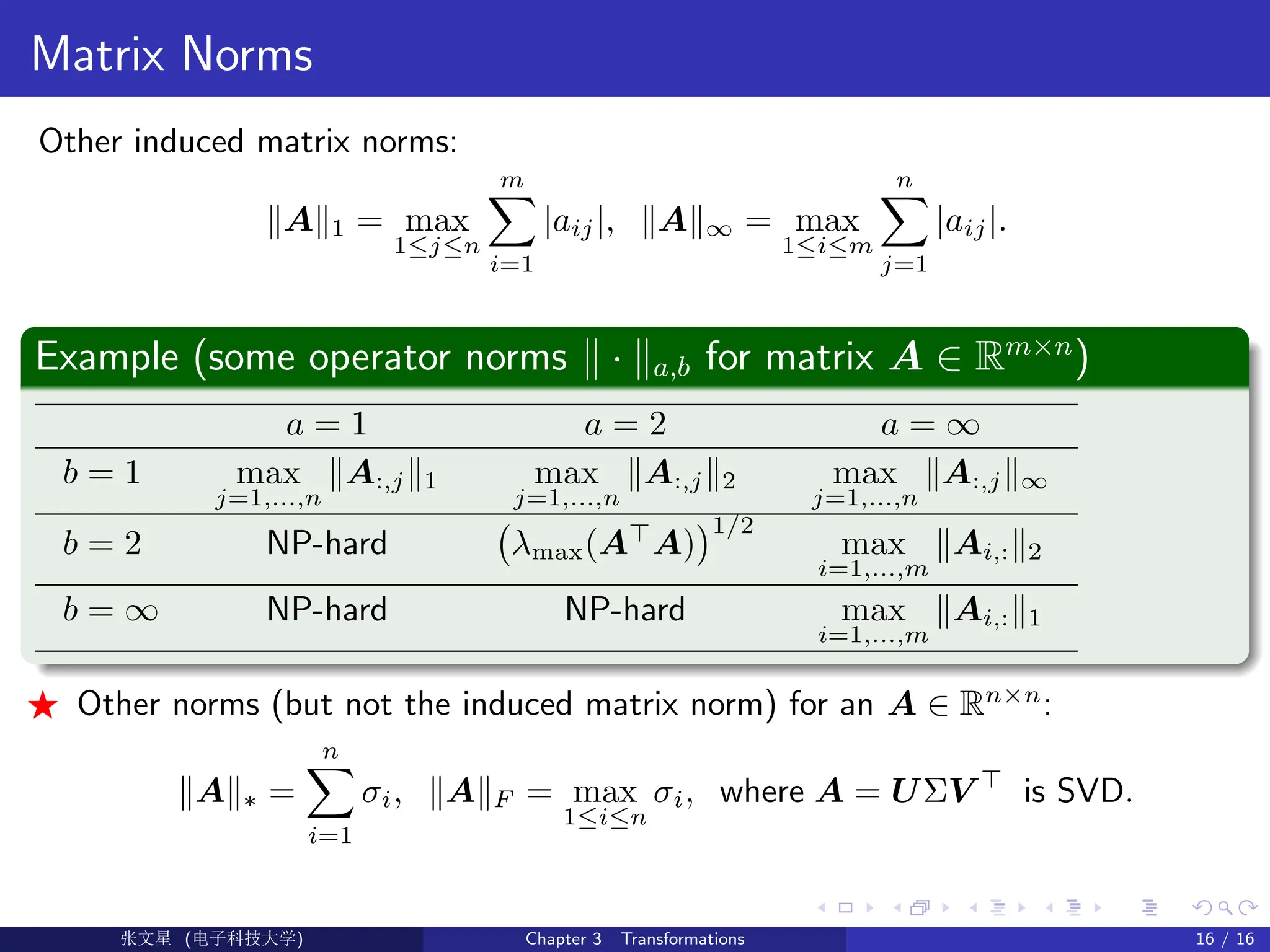
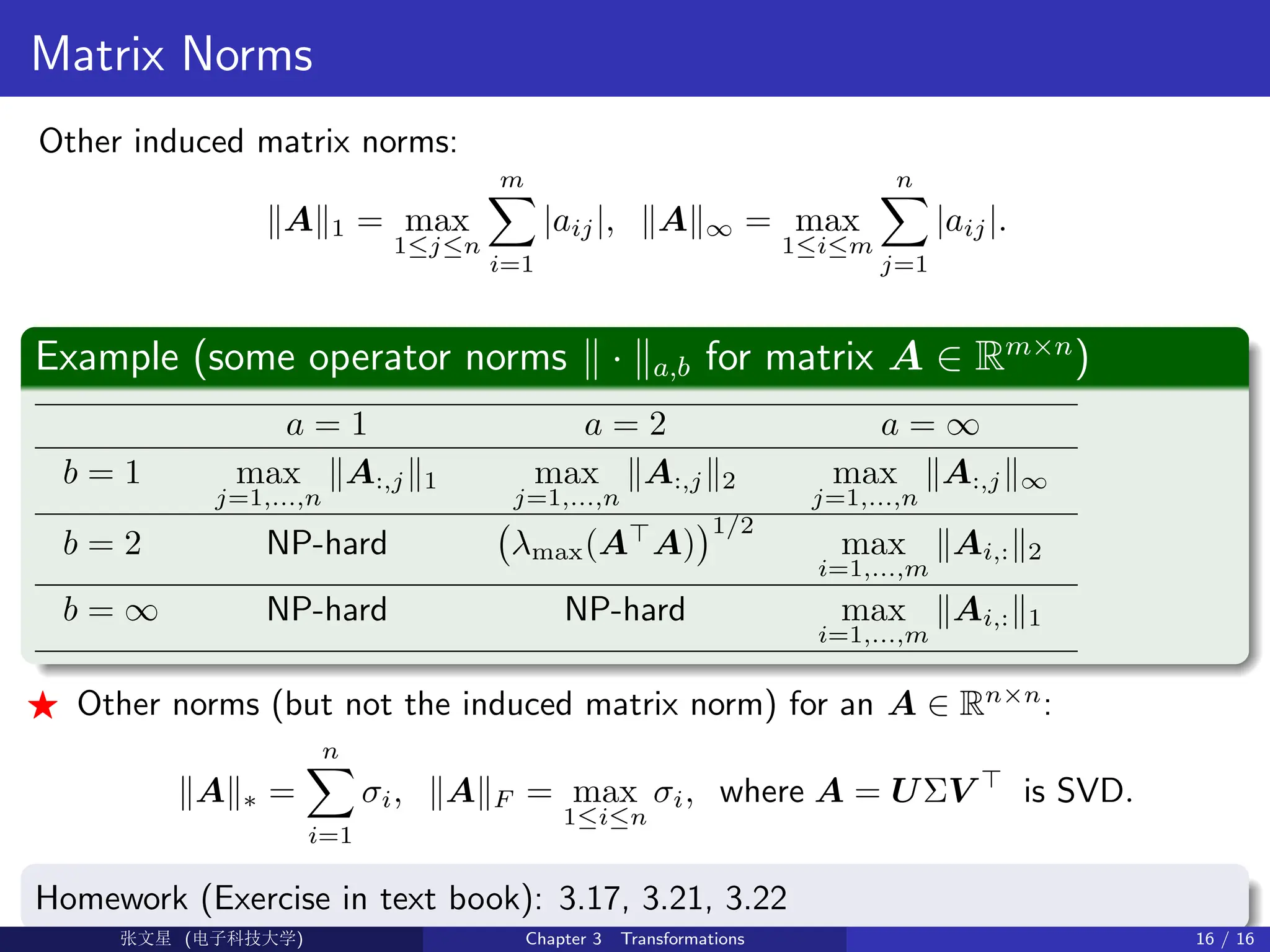
![Inner Products and Norms
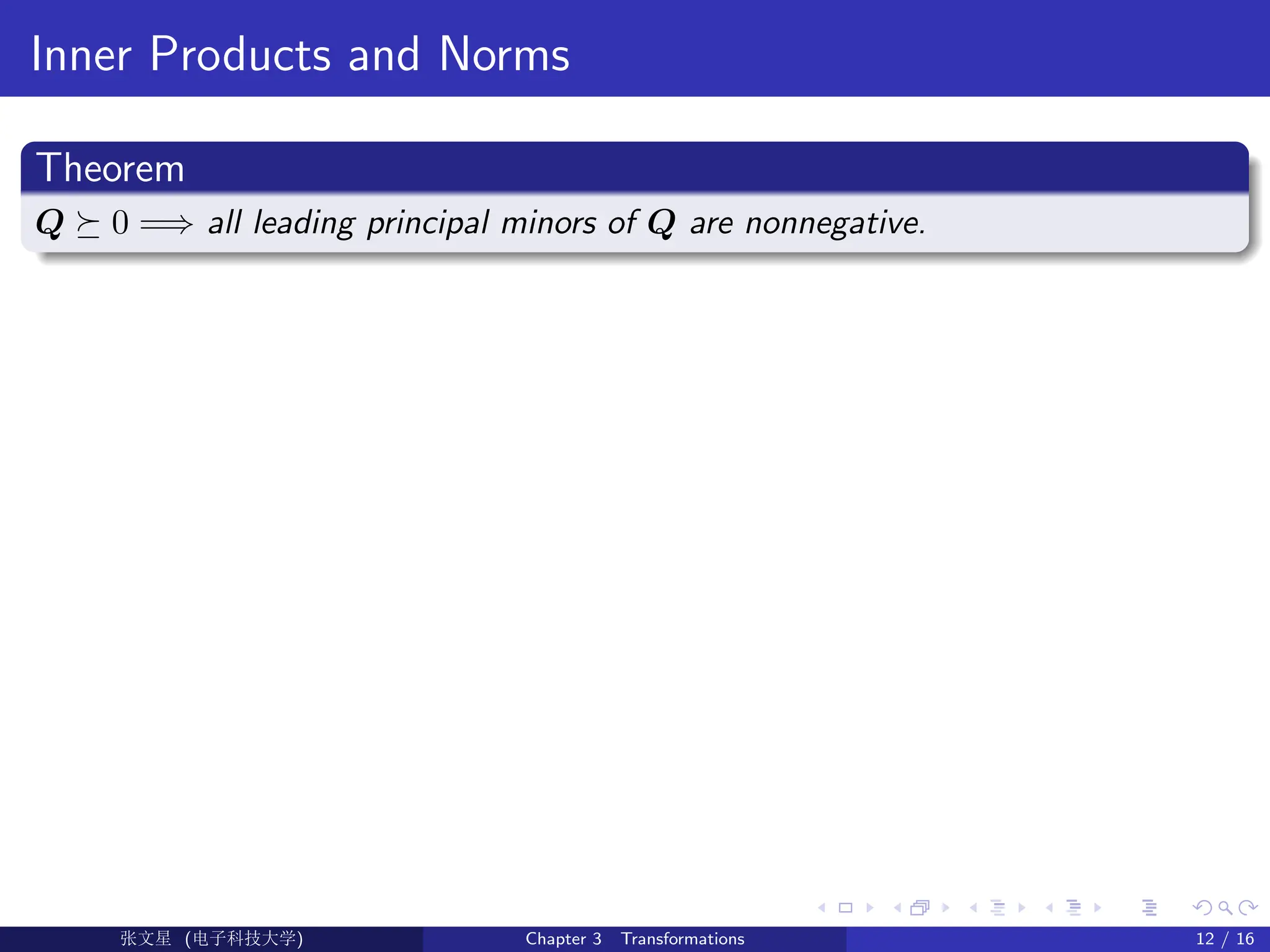
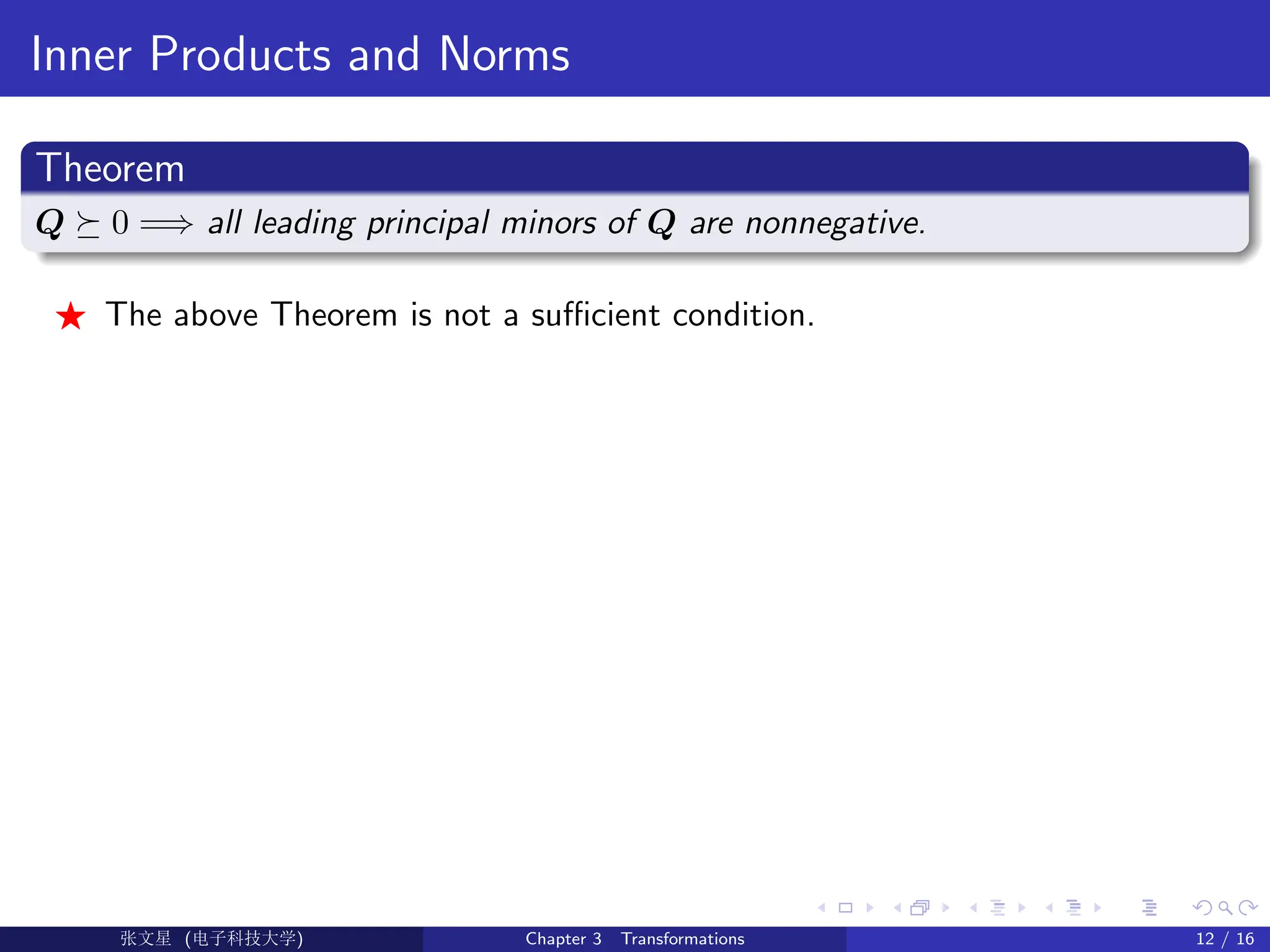
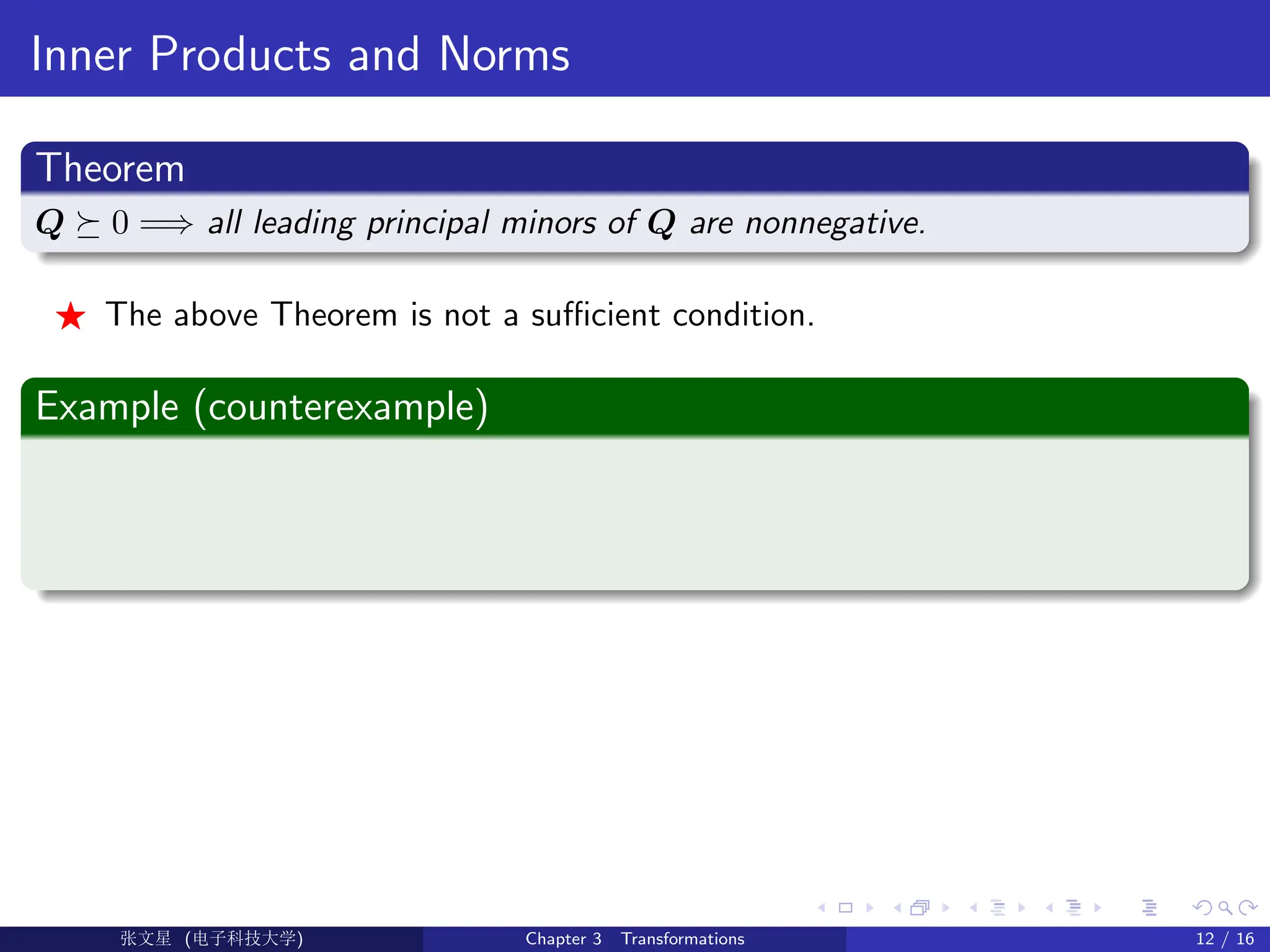
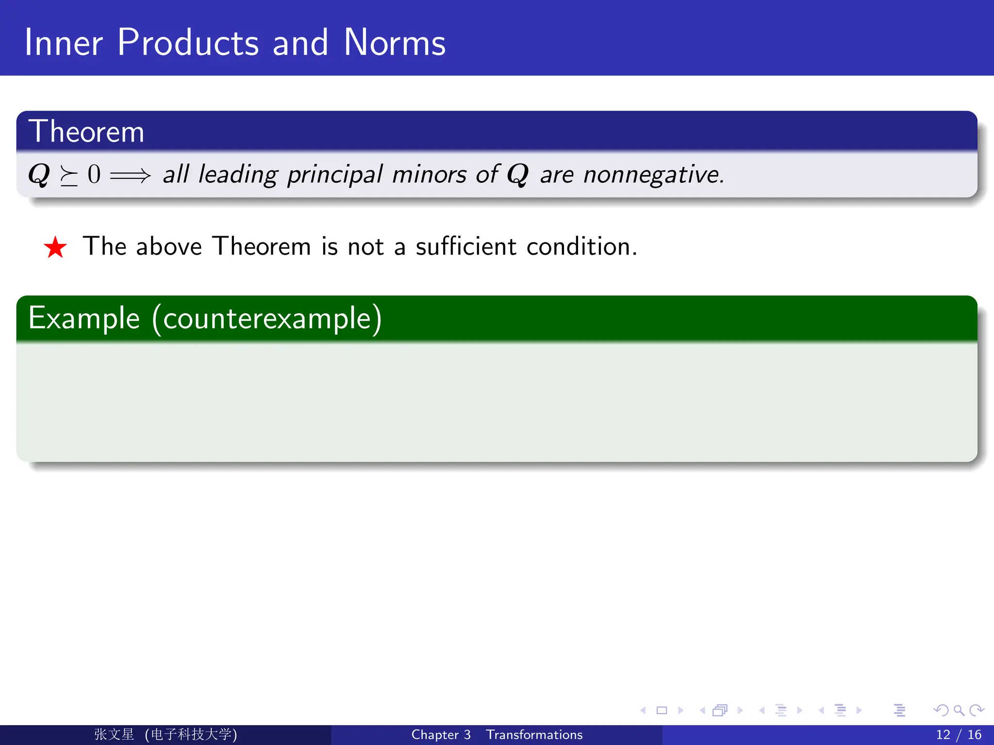
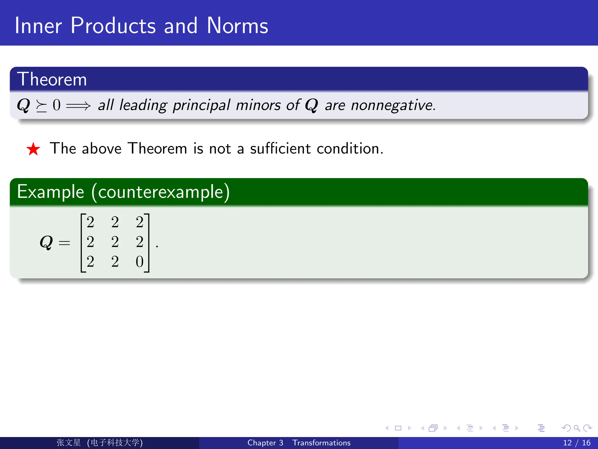
Theorem
Q 0 =⇒ all leading principal minors of Q are nonnegative.
F The above Theorem is not a sufficient condition.
Example (counterexample)
Q =
2 2 2
2 2 2
2 2 0
.
Although ∆1 = 2, ∆2 = 0 ∆3 = 0, Q 0.
(∵ x = [1, 1, −2]
⇔ x
Qx 0).
Ü©( (f‰EŒÆ) Chapter 3 Transformations 12 / 16](https://image.slidesharecdn.com/chapter3-251114130840-87080d8d/75/Introduction-to-Optimization-methods-lecture-1-67-2048.jpg)
![Inner Products and Norms
Theorem
Q 0 =⇒ all leading principal minors of Q are nonnegative.
F The above Theorem is not a sufficient condition.
Example (counterexample)
Q =
2 2 2
2 2 2
2 2 0
.
Although ∆1 = 2, ∆2 = 0 ∆3 = 0, Q 0.
(∵ x = [1, 1, −2]
⇔ x
Qx 0).
Theorem (positive semidefinite)
Ü©( (f‰EŒÆ) Chapter 3 Transformations 12 / 16](https://image.slidesharecdn.com/chapter3-251114130840-87080d8d/75/Introduction-to-Optimization-methods-lecture-1-68-2048.jpg)
![Inner Products and Norms
Theorem
Q 0 =⇒ all leading principal minors of Q are nonnegative.
F The above Theorem is not a sufficient condition.
Example (counterexample)
Q =
2 2 2
2 2 2
2 2 0
.
Although ∆1 = 2, ∆2 = 0 ∆3 = 0, Q 0.
(∵ x = [1, 1, −2]
⇔ x
Qx 0).
Theorem (positive semidefinite)
Q 0 ⇐⇒ all principal minors of Q are nonnegative.
Ü©( (f‰EŒÆ) Chapter 3 Transformations 12 / 16](https://image.slidesharecdn.com/chapter3-251114130840-87080d8d/75/Introduction-to-Optimization-methods-lecture-1-69-2048.jpg)
![Inner Products and Norms
Theorem
Q 0 =⇒ all leading principal minors of Q are nonnegative.
F The above Theorem is not a sufficient condition.
Example (counterexample)
Q =
2 2 2
2 2 2
2 2 0
.
Although ∆1 = 2, ∆2 = 0 ∆3 = 0, Q 0.
(∵ x = [1, 1, −2]
⇔ x
Qx 0).
Theorem (positive semidefinite)
Q 0 ⇐⇒ all principal minors of Q are nonnegative.
Q 0 ⇐⇒ all eigenvalues of Q are nonnegative.
Ü©( (f‰EŒÆ) Chapter 3 Transformations 12 / 16](https://image.slidesharecdn.com/chapter3-251114130840-87080d8d/75/Introduction-to-Optimization-methods-lecture-1-70-2048.jpg)
![Inner Products and Norms
Theorem
Q 0 =⇒ all leading principal minors of Q are nonnegative.
F The above Theorem is not a sufficient condition.
Example (counterexample)
Q =
2 2 2
2 2 2
2 2 0
.
Although ∆1 = 2, ∆2 = 0 ∆3 = 0, Q 0.
(∵ x = [1, 1, −2]
⇔ x
Qx 0).
Theorem (positive semidefinite)
Q 0 ⇐⇒ all principal minors of Q are nonnegative.
Q 0 ⇐⇒ all eigenvalues of Q are nonnegative.
proof in linear algebra textbook.
Ü©( (f‰EŒÆ) Chapter 3 Transformations 12 / 16](https://image.slidesharecdn.com/chapter3-251114130840-87080d8d/75/Introduction-to-Optimization-methods-lecture-1-71-2048.jpg)