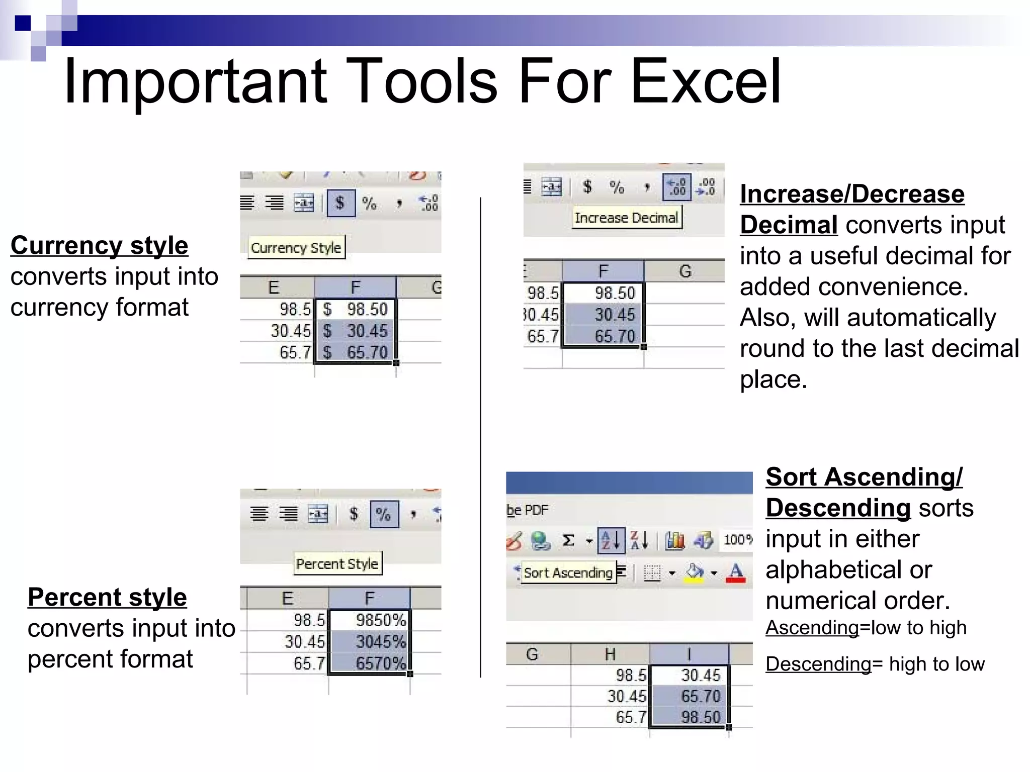
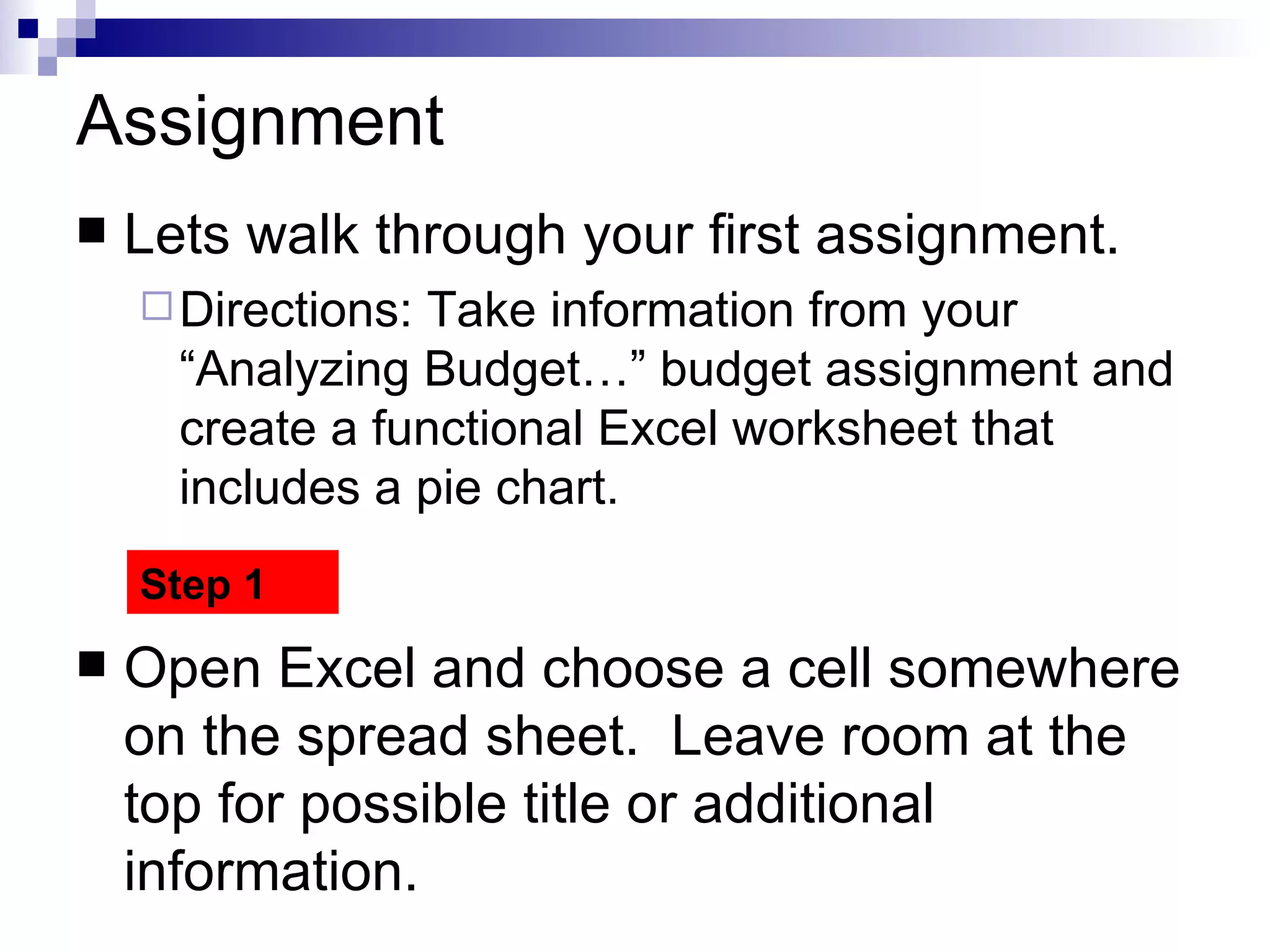
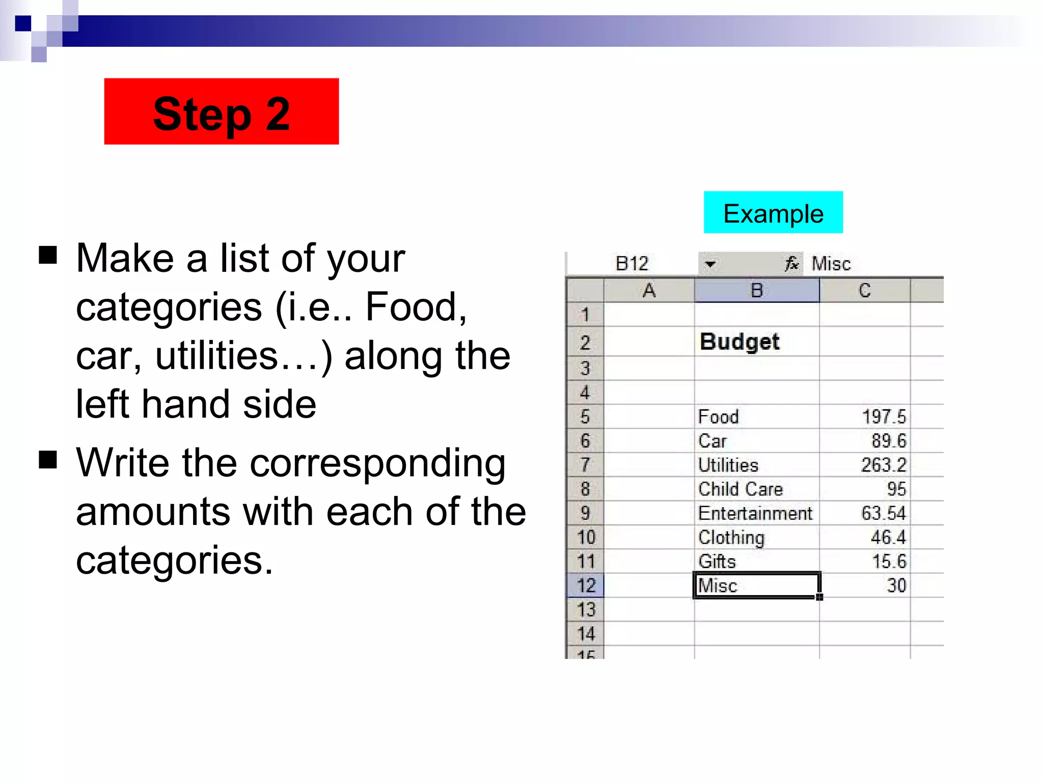
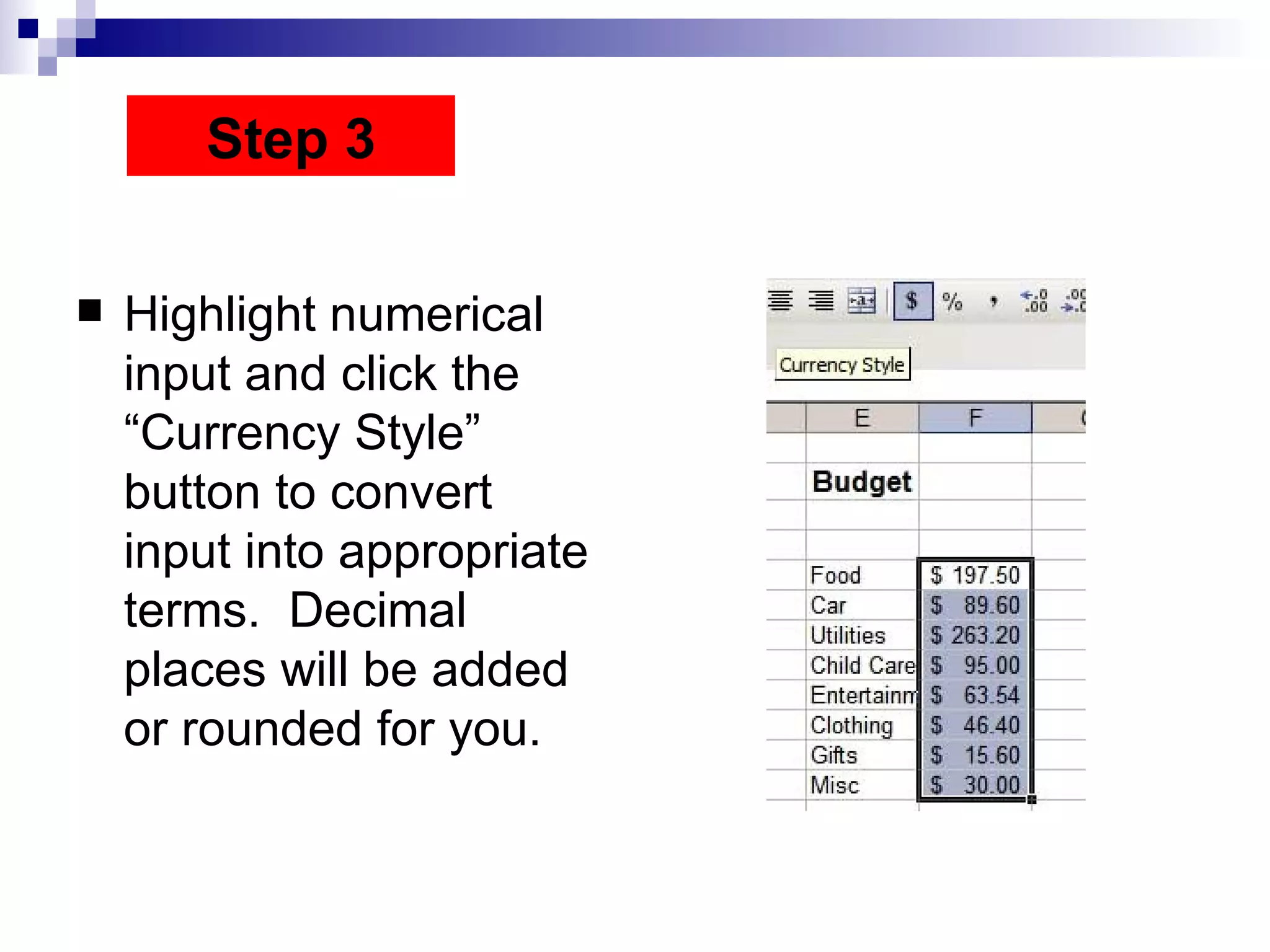
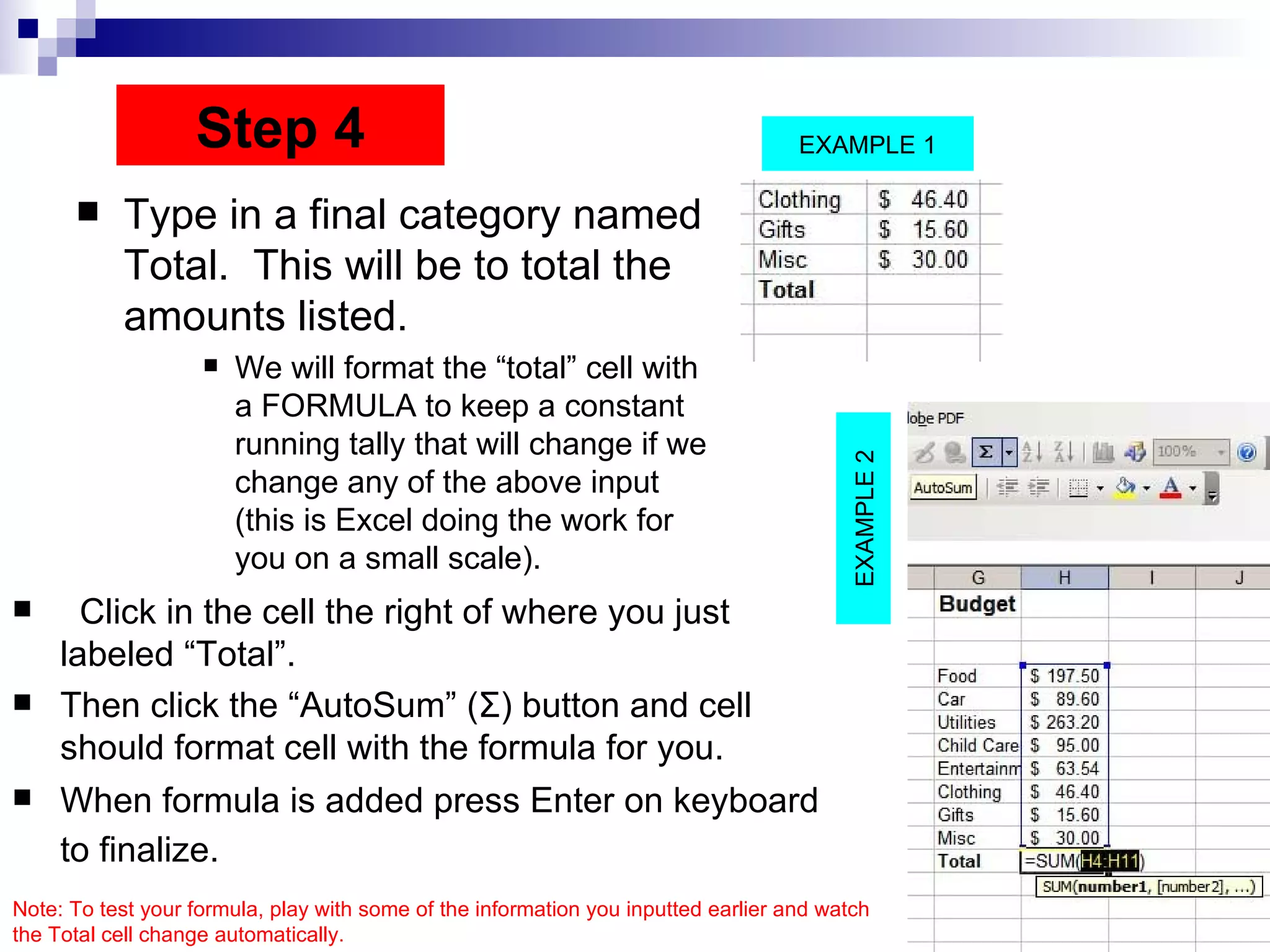
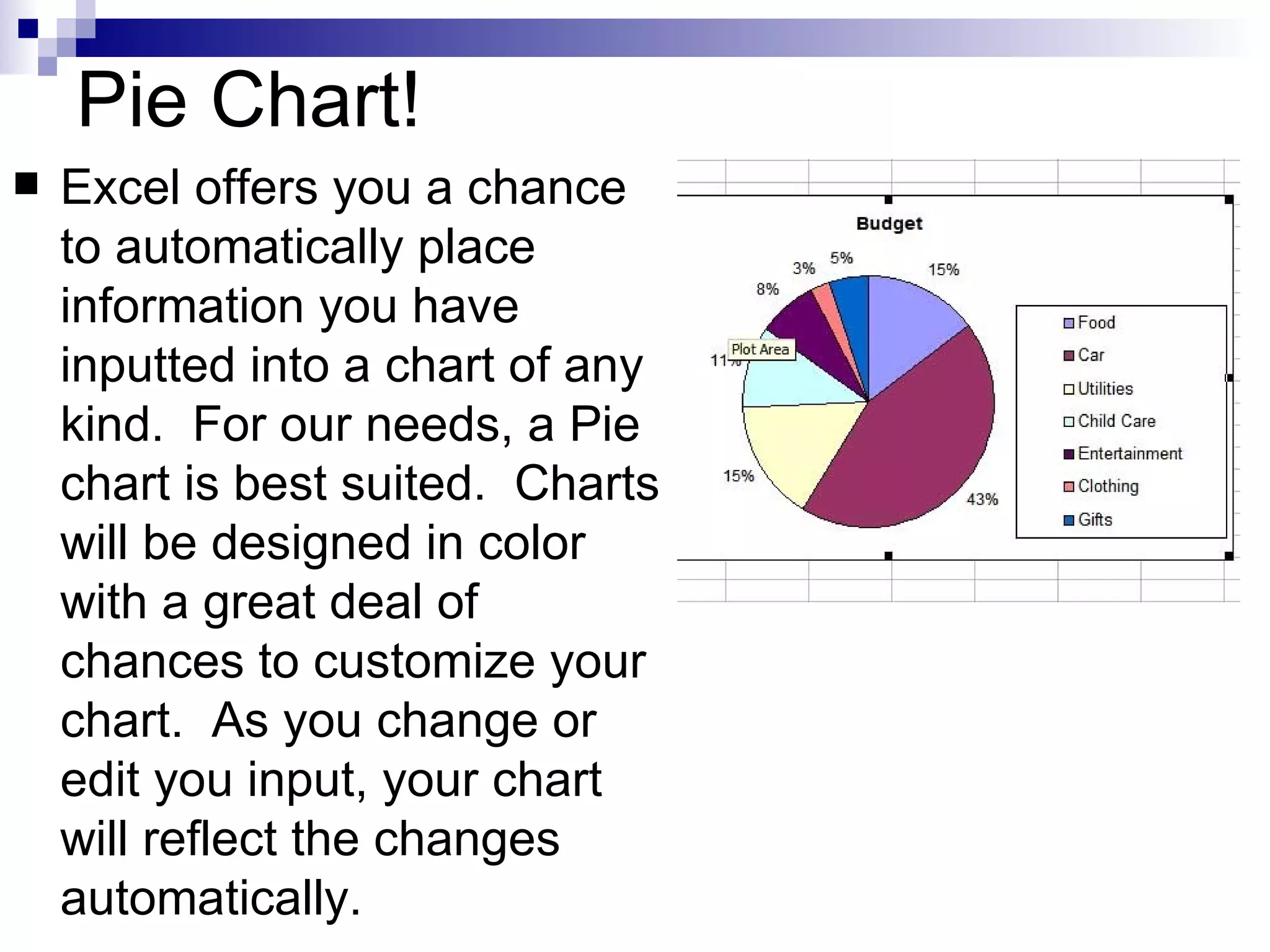
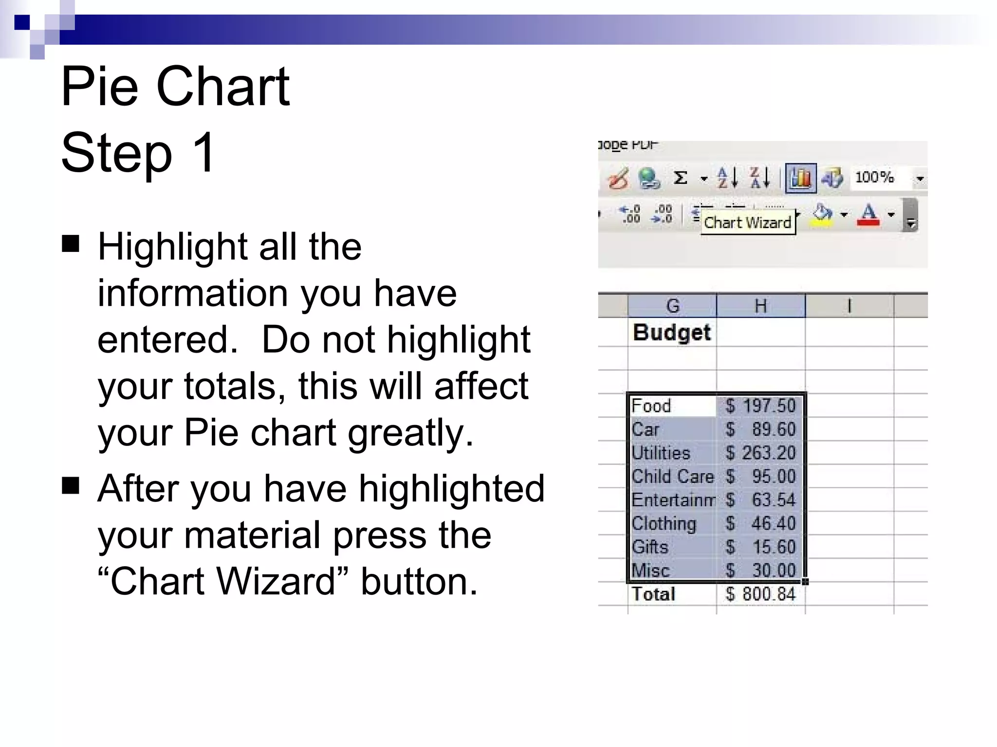
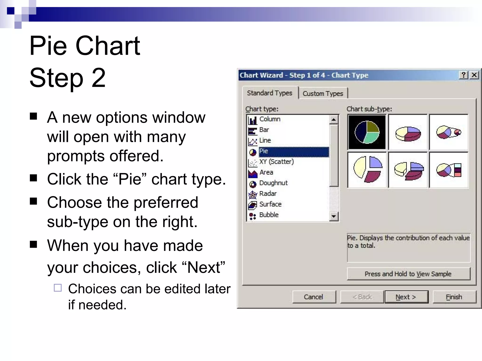
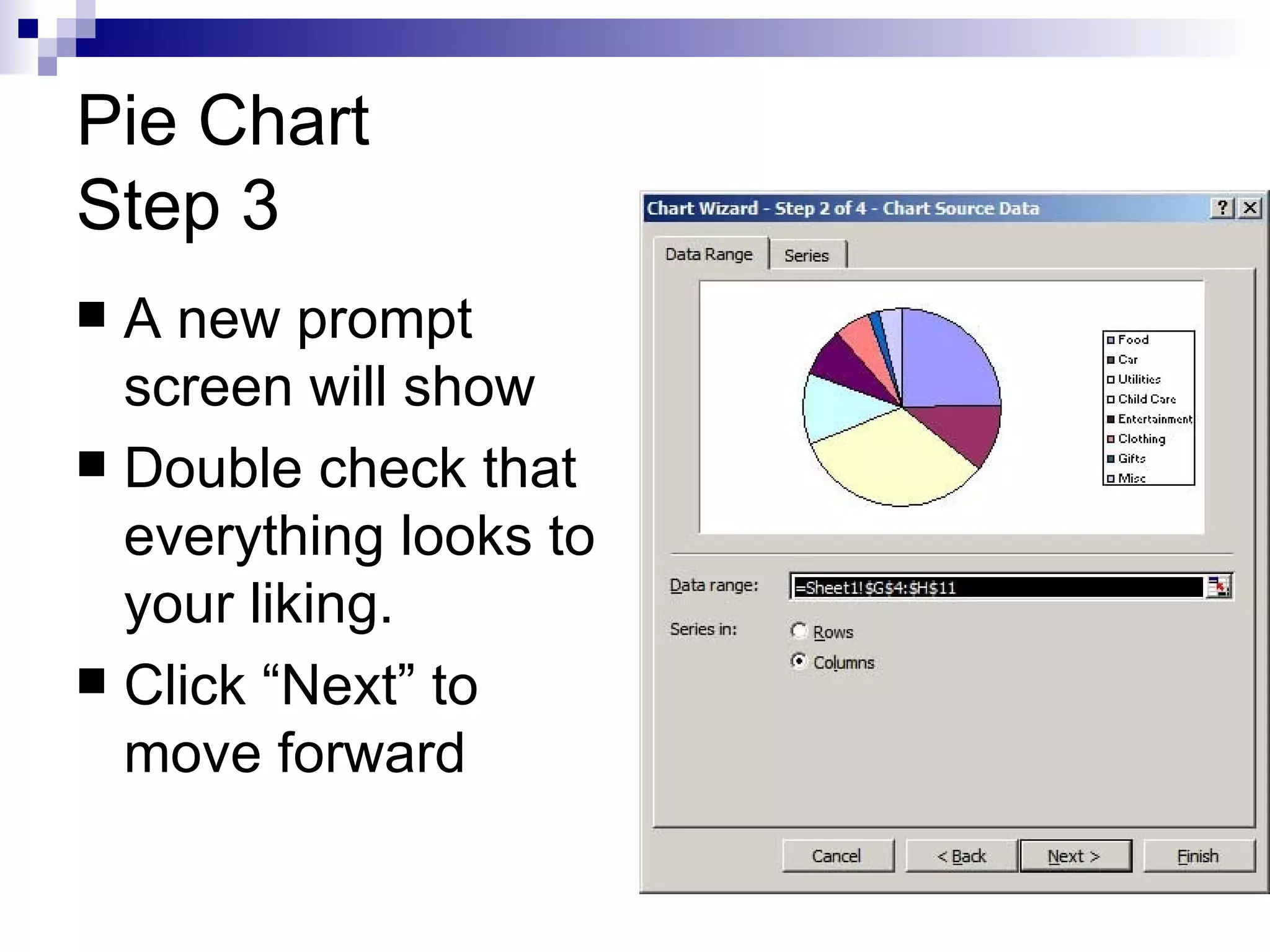
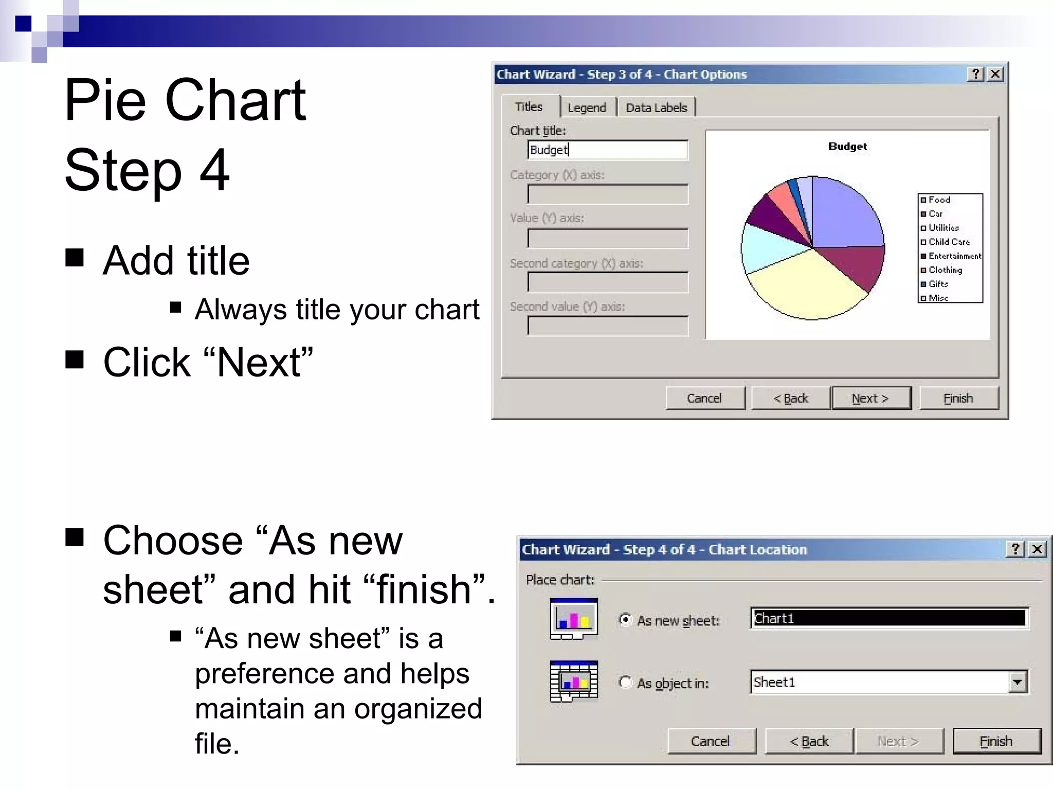
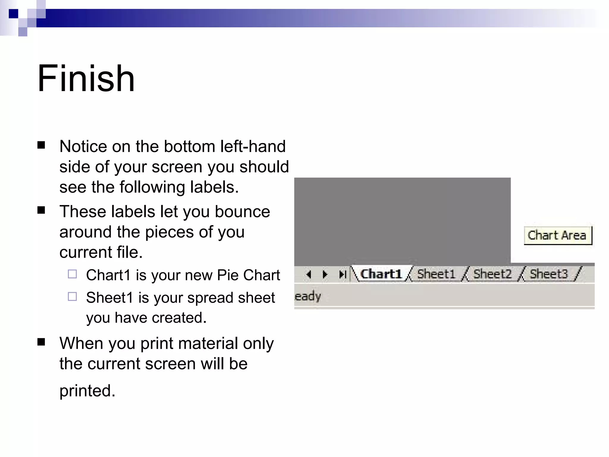
Create A Chart In Excel

Create A Chart In Excel

• 1.
  Create A Chartin Excel Consumer Education Mr. Lowery
• 2.
  Welcome To Excel…itsfun! Excel can be a helpful tool for organizing small, large, ongoing, and or repeating batches of information. If you know it well enough it can do the work for you! Which is nice.
• 3.
  Let’s begin Clickthe GREEN logo Notice the many tools along the top. Many similar to WORD
• 4.
  Important Tools ForExcel Currency style converts input into currency format Sort Ascending/ Descending sorts input in either alphabetical or numerical order. Ascending =low to high Descending = high to low Increase/Decrease Decimal converts input into a useful decimal for added convenience. Also, will automatically round to the last decimal place. Percent style converts input into percent format
• 5.
  Hints!!! Trust me…CTRL + Z … Undo the last thing you did. You can hit this as many times as you want to get back to the desired spot. ESC while working in a cell, the ESC key will remove you without changing the first input.
• 6.
  Assignment Lets walkthrough your first assignment. Directions: Take information from your “Analyzing Budget…” budget assignment and create a functional Excel worksheet that includes a pie chart. Open Excel and choose a cell somewhere on the spread sheet. Leave room at the top for possible title or additional information. Step 1
• 7.
  Make a listof your categories (i.e.. Food, car, utilities…) along the left hand side Write the corresponding amounts with each of the categories. Step 2 Example
• 8.
  Highlight numerical inputand click the “Currency Style” button to convert input into appropriate terms. Decimal places will be added or rounded for you. Step 3
• 9.
  Type in afinal category named Total. This will be to total the amounts listed. We will format the “total” cell with a FORMULA to keep a constant running tally that will change if we change any of the above input (this is Excel doing the work for you on a small scale). Click in the cell the right of where you just labeled “Total”. Then click the “AutoSum” ( Σ ) button and cell should format cell with the formula for you. When formula is added press Enter on keyboard to finalize. Step 4 EXAMPLE 2 EXAMPLE 1 Note: To test your formula, play with some of the information you inputted earlier and watch the Total cell change automatically.
• 10.
  Pie Chart! Exceloffers you a chance to automatically place information you have inputted into a chart of any kind. For our needs, a Pie chart is best suited. Charts will be designed in color with a great deal of chances to customize your chart. As you change or edit you input, your chart will reflect the changes automatically.
• 11.
  Pie Chart Step 1 Highlight all the information you have entered. Do not highlight your totals, this will affect your Pie chart greatly. After you have highlighted your material press the “Chart Wizard” button.
• 12.
  Pie Chart Step2 A new options window will open with many prompts offered. Click the “Pie” chart type. Choose the preferred sub-type on the right. When you have made your choices, click “Next” Choices can be edited later if needed.
• 13.
  Pie Chart Step3 A new prompt screen will show Double check that everything looks to your liking. Click “Next” to move forward
• 14.
  Pie Chart Step4 Add title Always title your chart Click “Next” Choose “As new sheet” and hit “finish”. “ As new sheet” is a preference and helps maintain an organized file.
• 15.
  Finish Notice onthe bottom left-hand side of your screen you should see the following labels. These labels let you bounce around the pieces of you current file. Chart1 is your new Pie Chart Sheet1 is your spread sheet you have created . When you print material only the current screen will be printed.