Download as PDF, PPTX

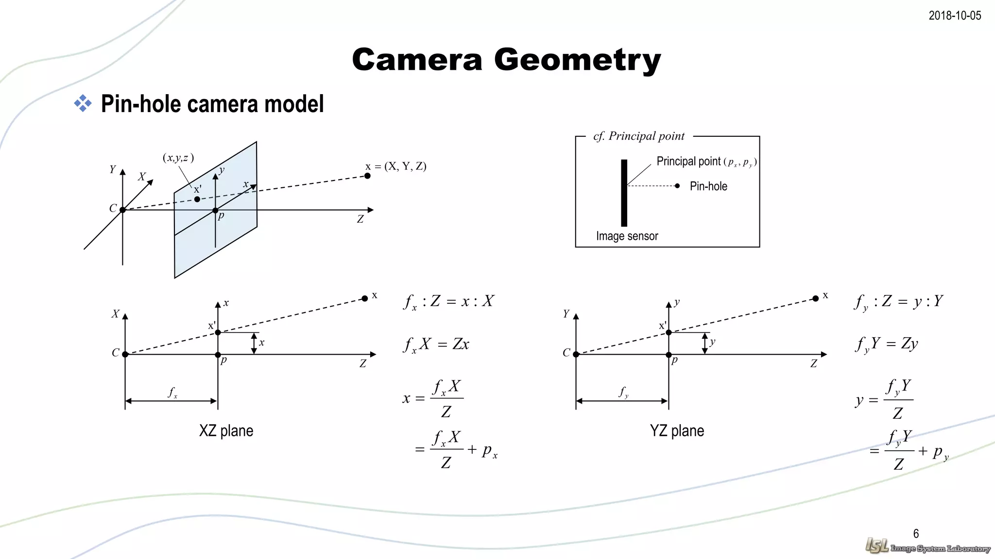


![2018-10-05
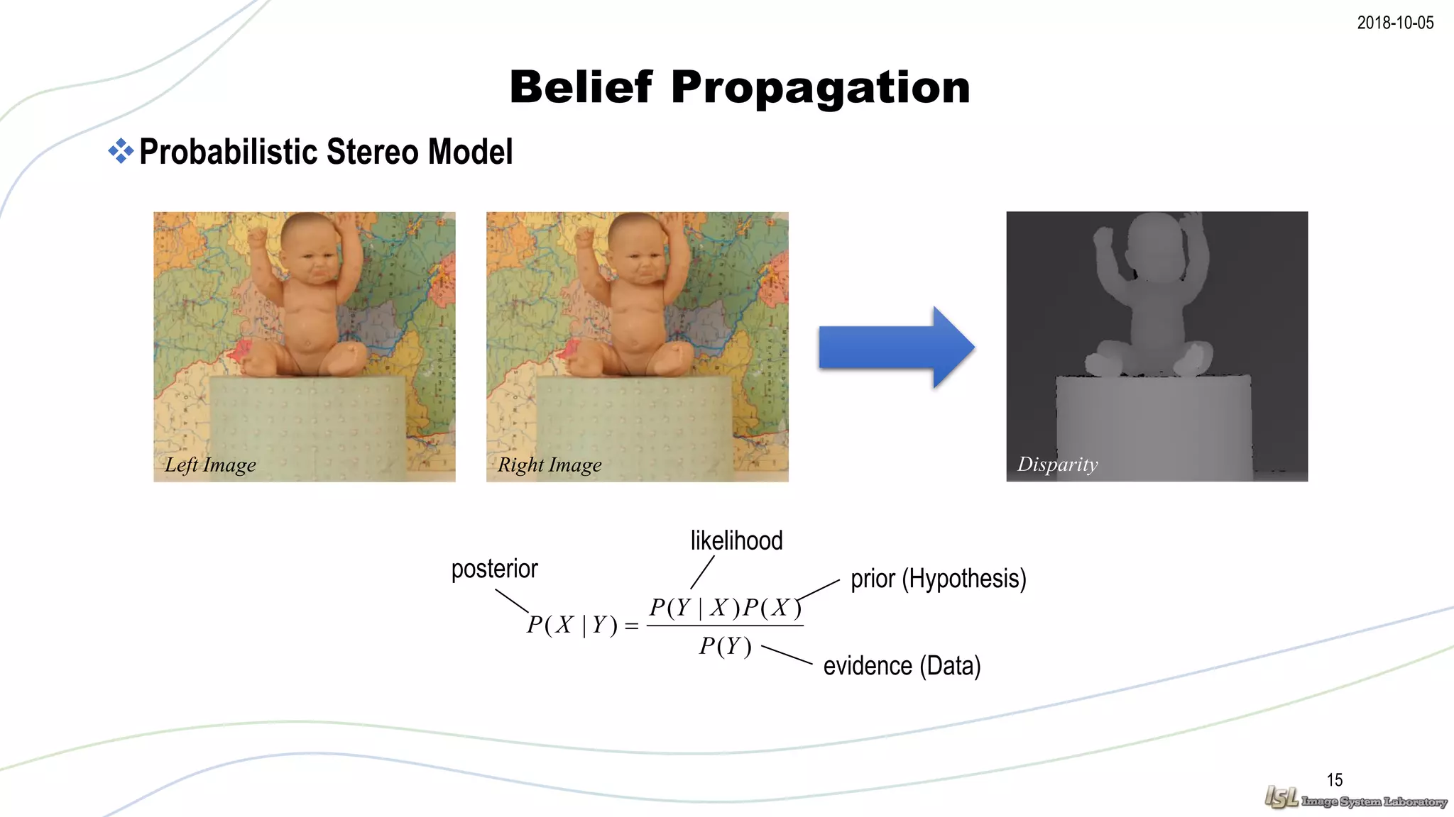
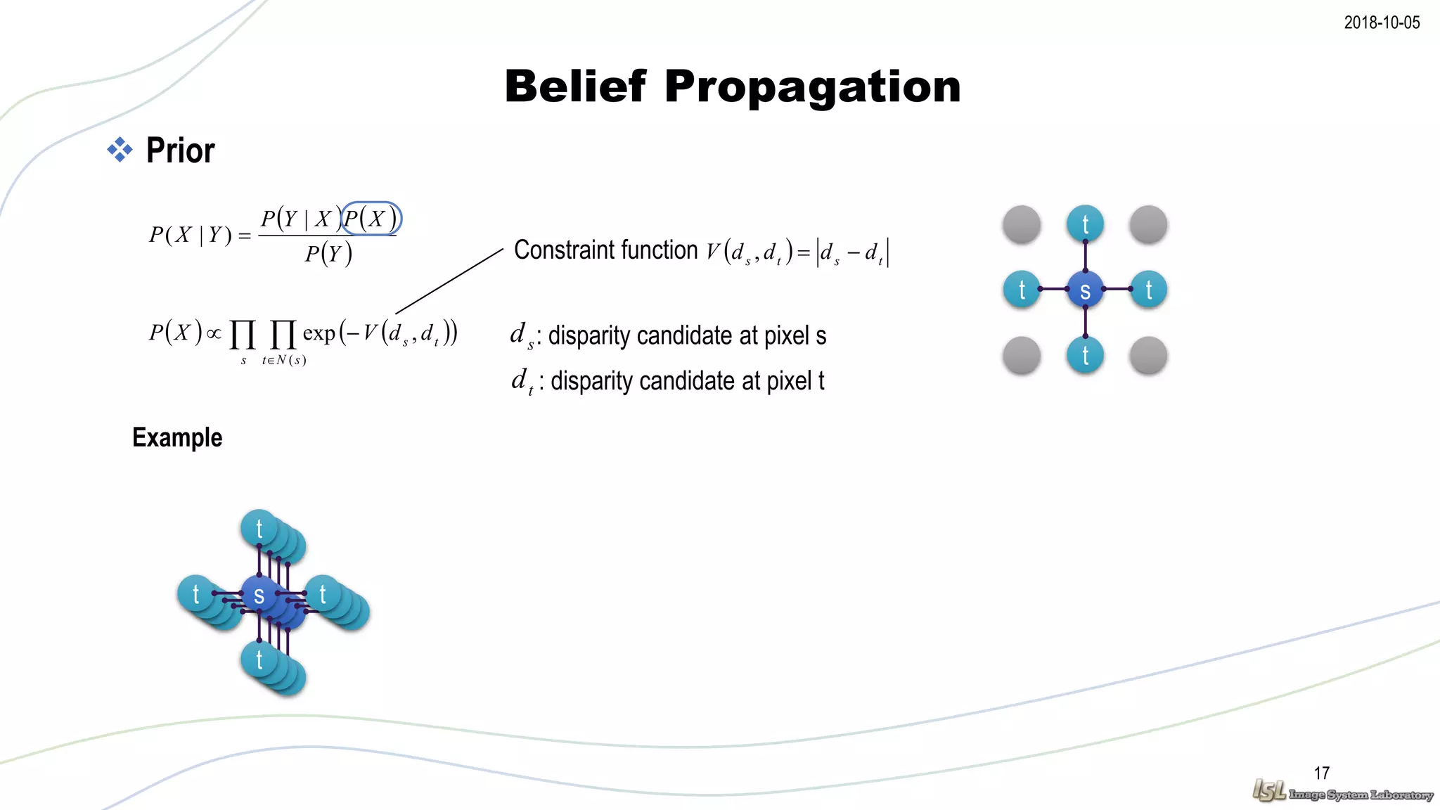
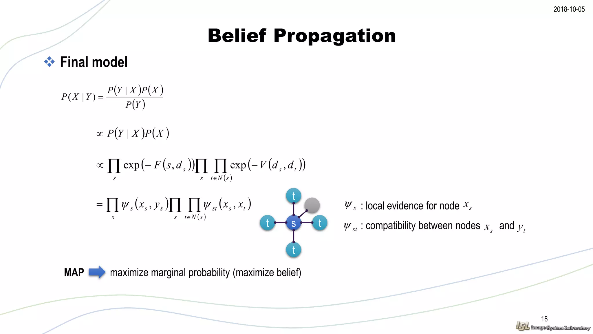
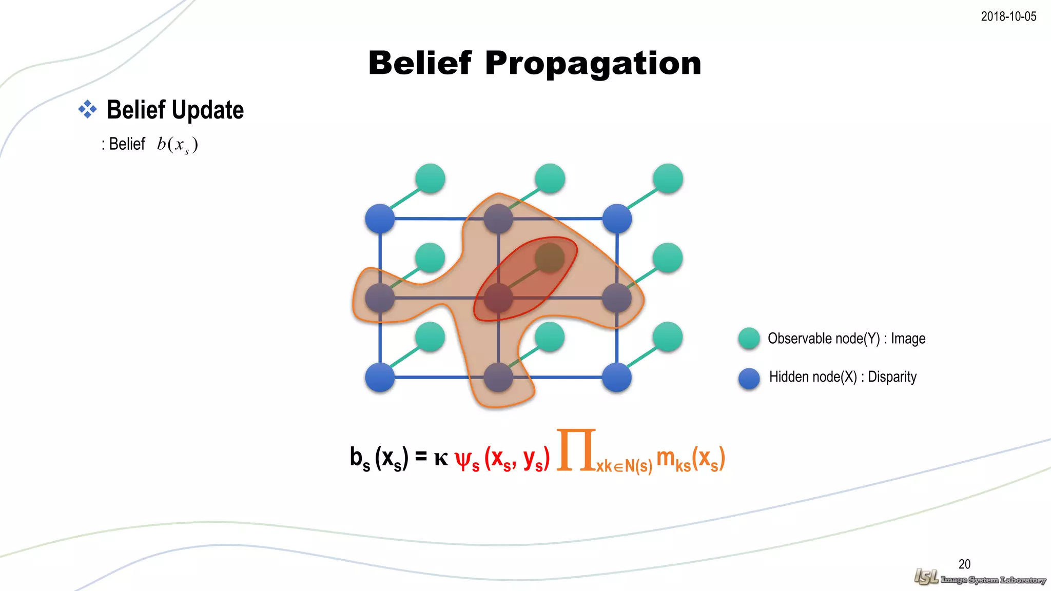
Belief Propagation
19
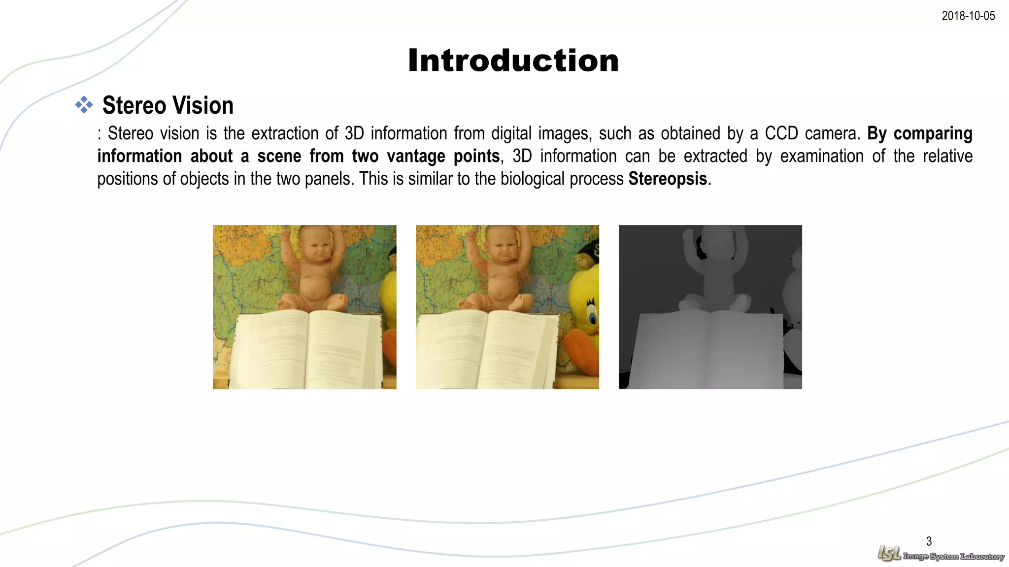
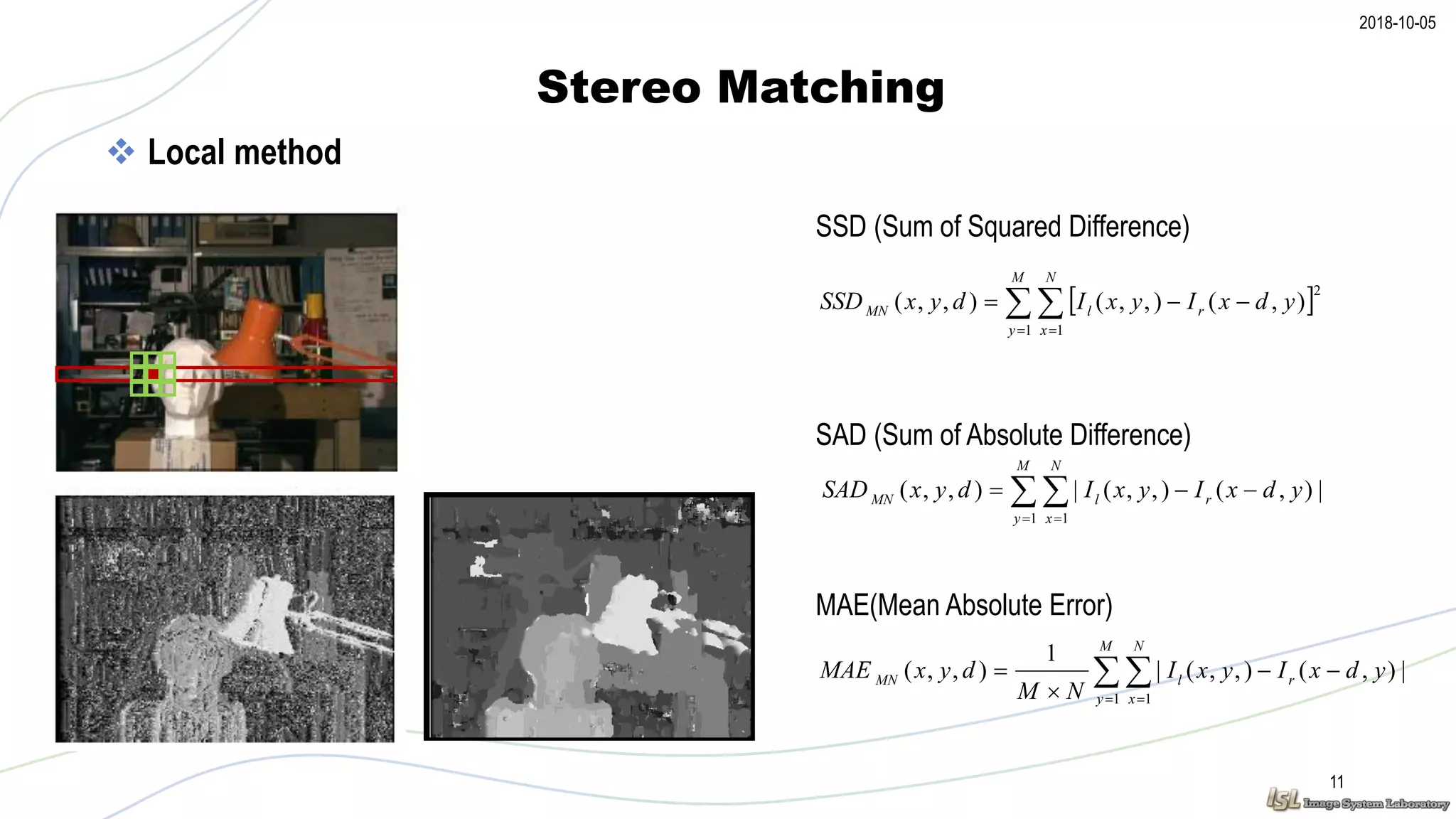
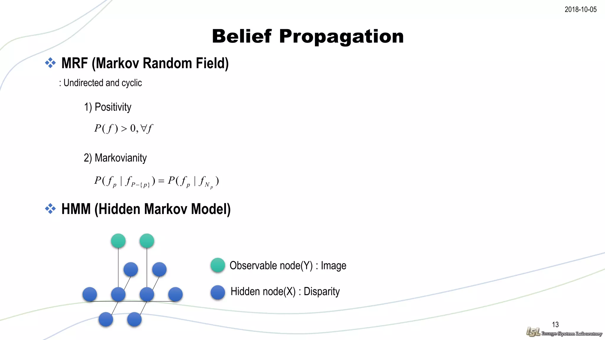
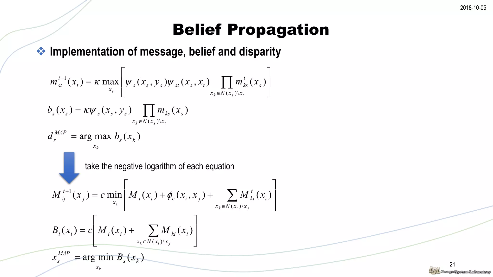
Observable node(Y) : Image
Hidden node(X) : Disparity
Message Passing
mst(xt) = κmax(xs) [s(xs, ys) st(xs, xt) xkN(s)t mks(xs)]
: Message stm sx txfrom to
ms(xs) : local evidence](https://image.slidesharecdn.com/stereomatchingusingbeliefpropagationalgorithm-181005080850/75/Stereo-matching-using-belief-propagation-algorithm-19-2048.jpg)
![2018-10-05
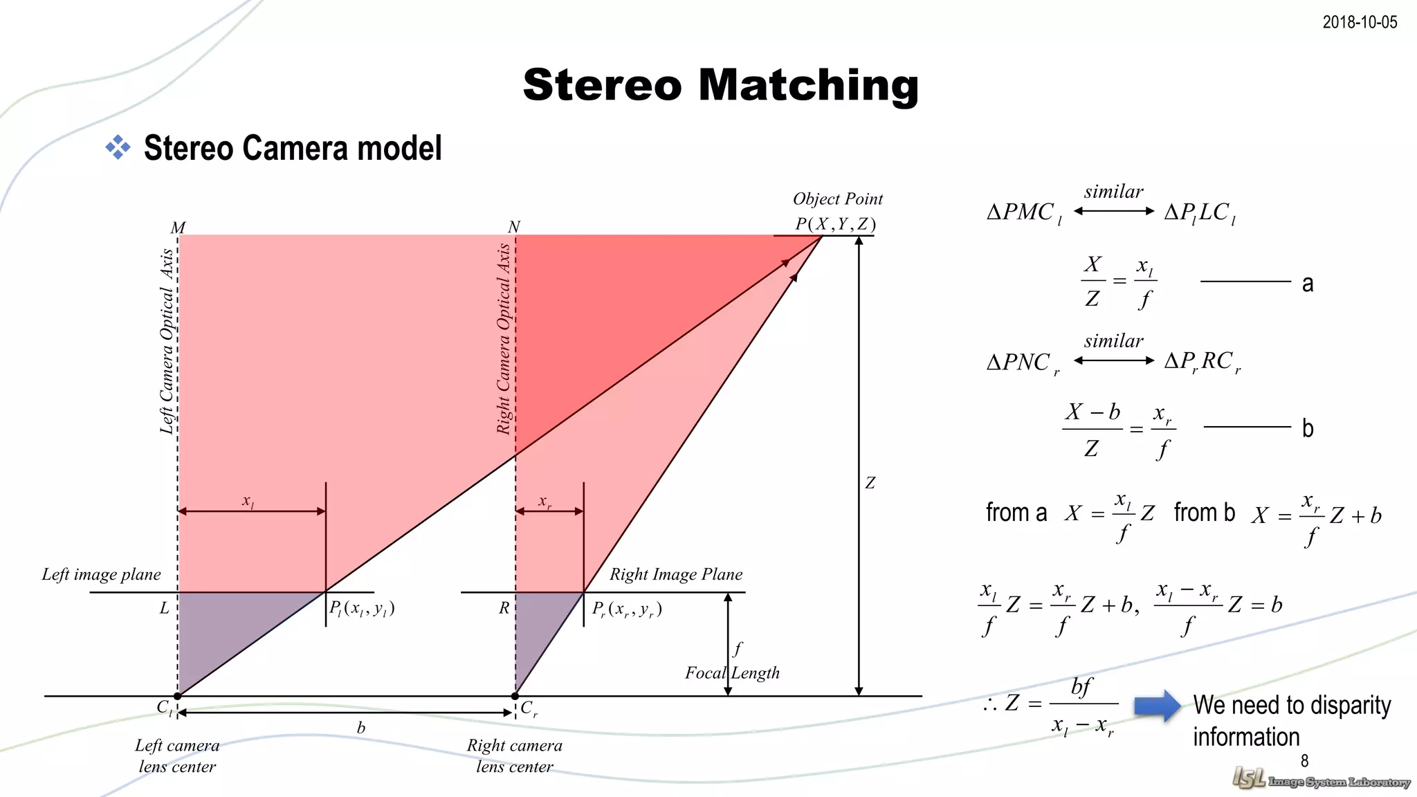
Belief Propagation
22
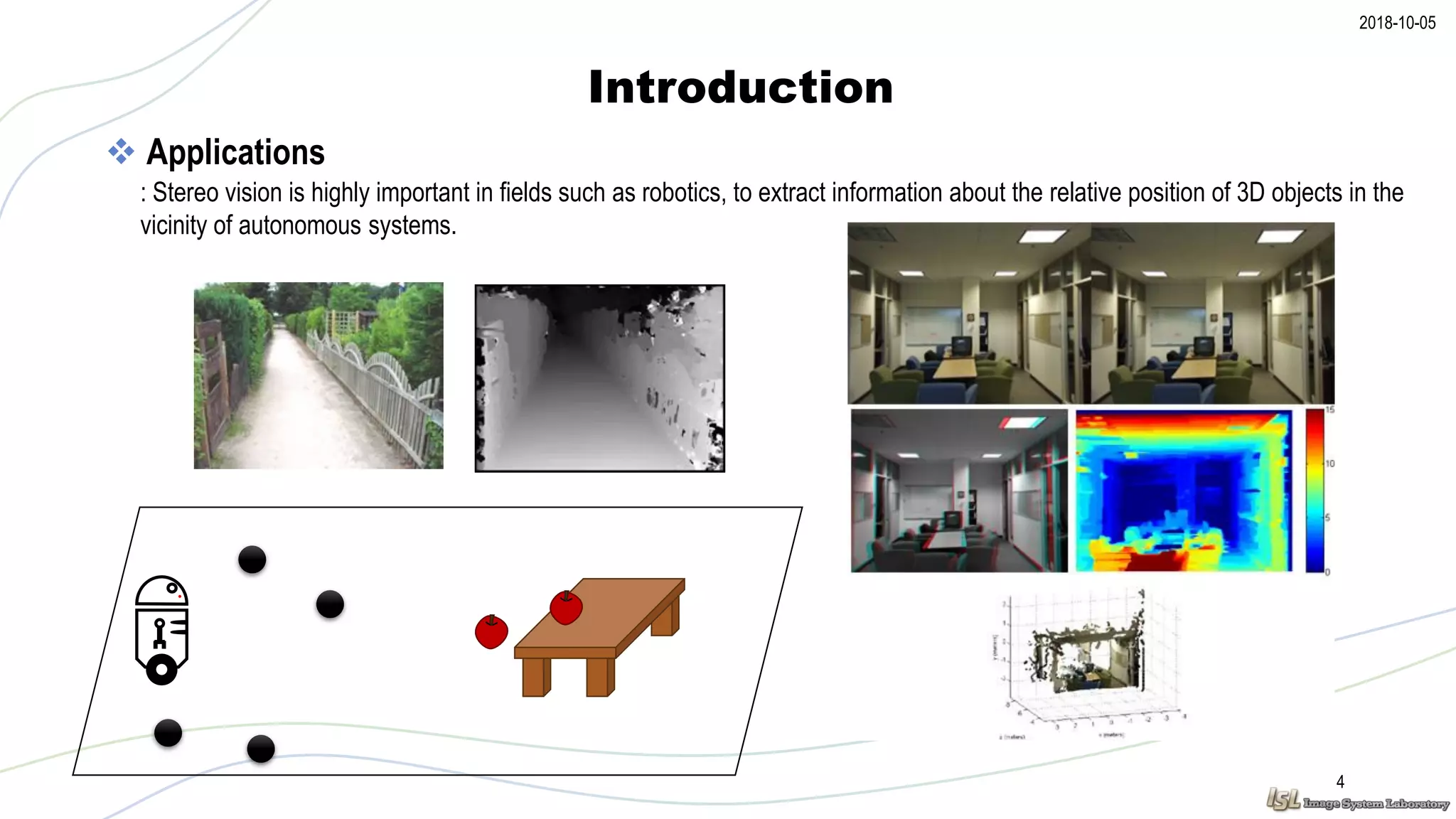
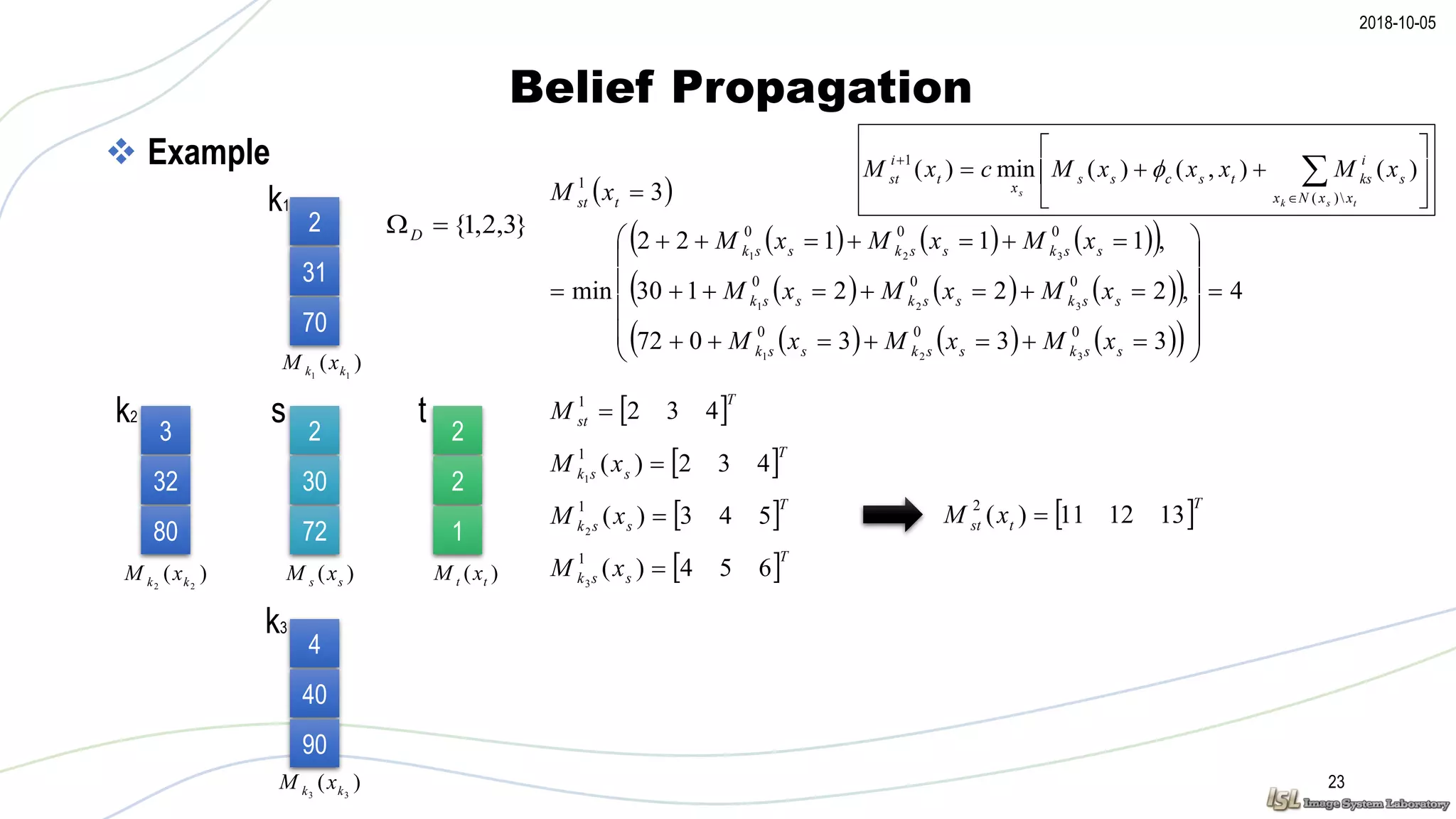
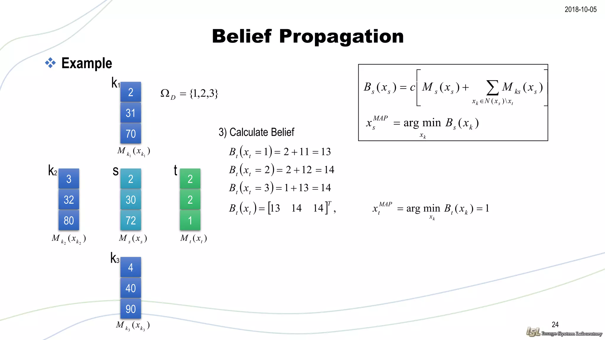
Example
T
ssksskssk
T
tst
xMxMxM
xM
]000[
000
000
0
321
1) Initialize
k1
2
333272
,222130
,11102
min
1
000
000
000
1
321
321
321
ssksskssk
ssksskssk
ssksskssk
tst
xMxMxM
xMxMxM
xMxMxM
xM
3
333172
,222030
,11112
min
2
000
000
000
1
321
321
321
ssksskssk
ssksskssk
ssksskssk
tst
xMxMxM
xMxMxM
xMxMxM
xM
2) Update
2
2
1
2
30
72
2
31
70
4
40
90
ts
k3
)( tt xM)( ss xM
)( 11 kk xM
)( 33 kk xM
}3,2,1{D
3
32
80
k2
)( 22 kk xM
tsk
s
xxNx
s
i
kstscss
x
t
i
st xMxxxMcxM
)(
1
)(),()(min)(
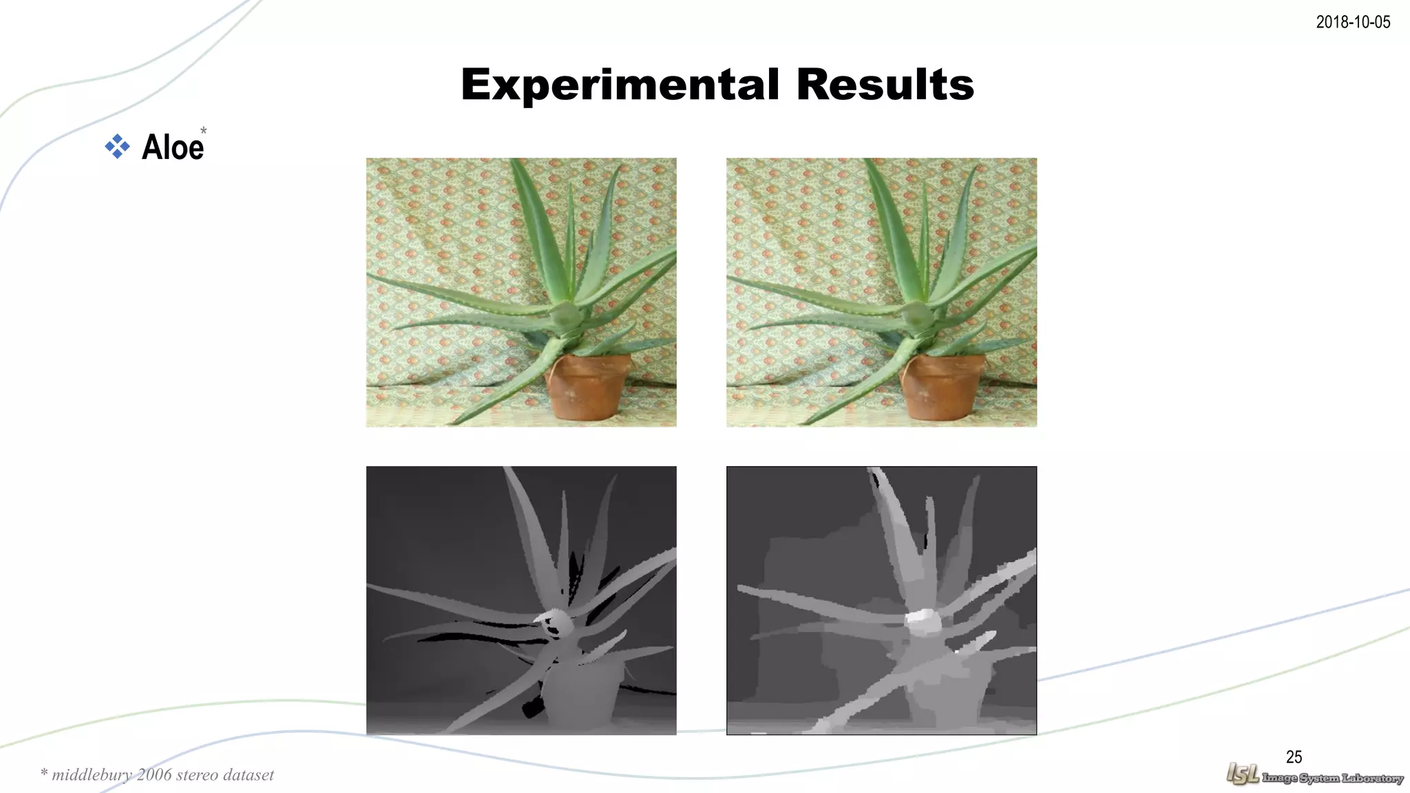
Left image
Right image](https://image.slidesharecdn.com/stereomatchingusingbeliefpropagationalgorithm-181005080850/75/Stereo-matching-using-belief-propagation-algorithm-22-2048.jpg)
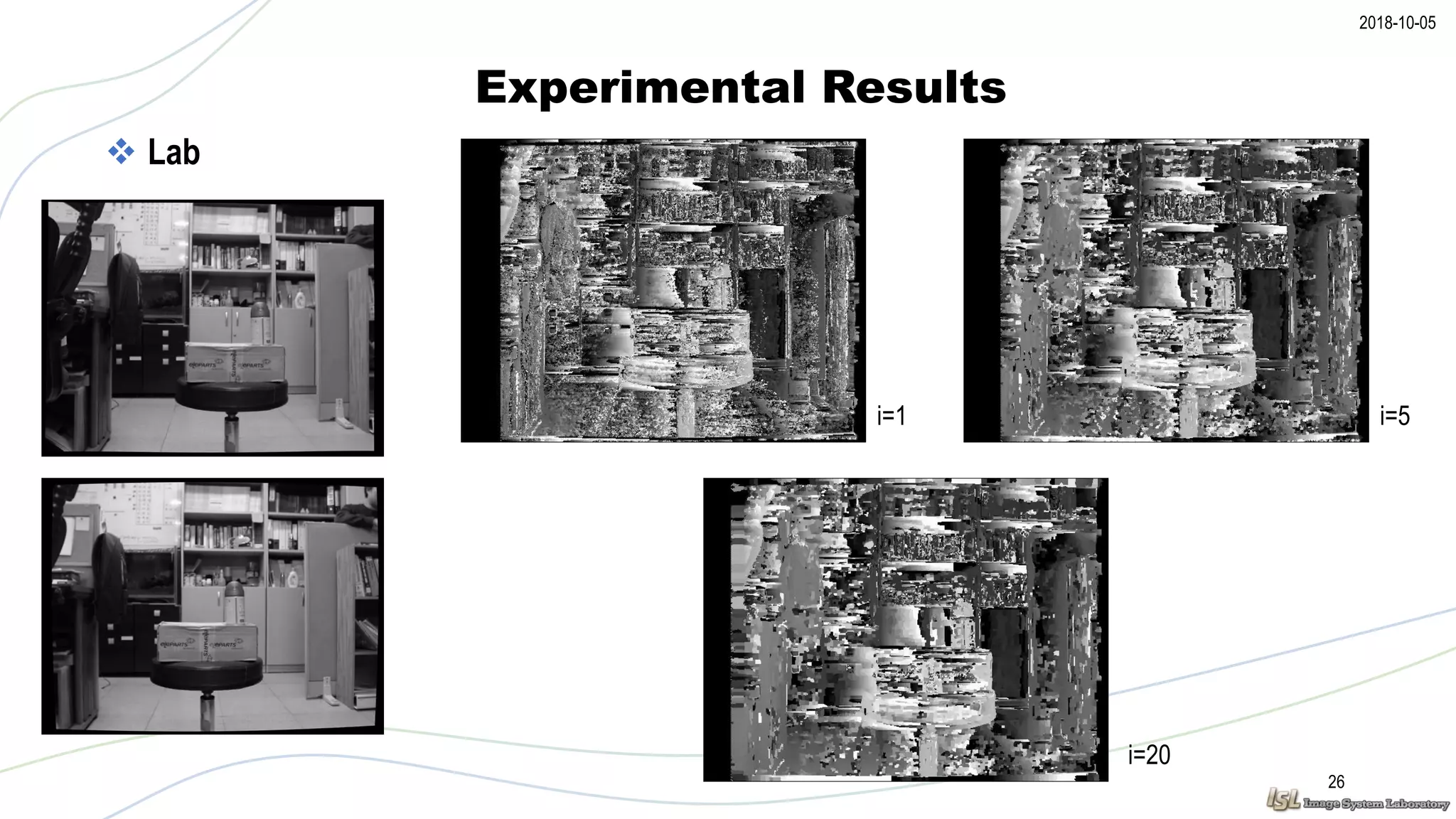


The document discusses stereo vision and the belief propagation algorithm applied to stereo matching. It explains camera geometry, with an emphasis on the pin-hole model, epipolar geometry, and challenges in correspondence problems, along with local and global methods for stereo matching. The belief propagation technique is detailed with respect to message passing and estimating disparity using probabilistic models.


![Vibe Coding vs. Spec-Driven Development [Free Meetup]](https://cdn.slidesharecdn.com/ss_thumbnails/vibecodingvsspecdrivendevelopment-251209105622-43f455e7-thumbnail.jpg?width=640&height=640&fit=bounds)
