Road Map
• Basicconcepts
• Decision tree induction
• Evaluation of classifiers
• Naïve Bayesian classification
• Naïve Bayes for text classification
• Support vector machines
• Linear regression and gradient descent
• Neural networks
• K-nearest neighbor
• Ensemble methods
• Summary
2
3.
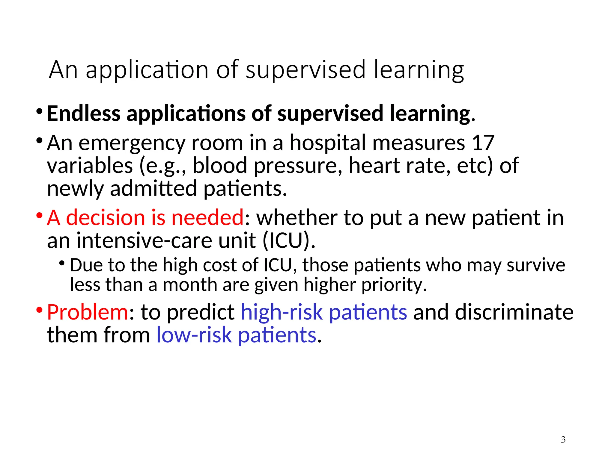
An application ofsupervised learning
•Endless applications of supervised learning.
•An emergency room in a hospital measures 17
variables (e.g., blood pressure, heart rate, etc) of
newly admitted patients.
•A decision is needed: whether to put a new patient in
an intensive-care unit (ICU).
• Due to the high cost of ICU, those patients who may survive
less than a month are given higher priority.
•Problem: to predict high-risk patients and discriminate
them from low-risk patients.
3
4.
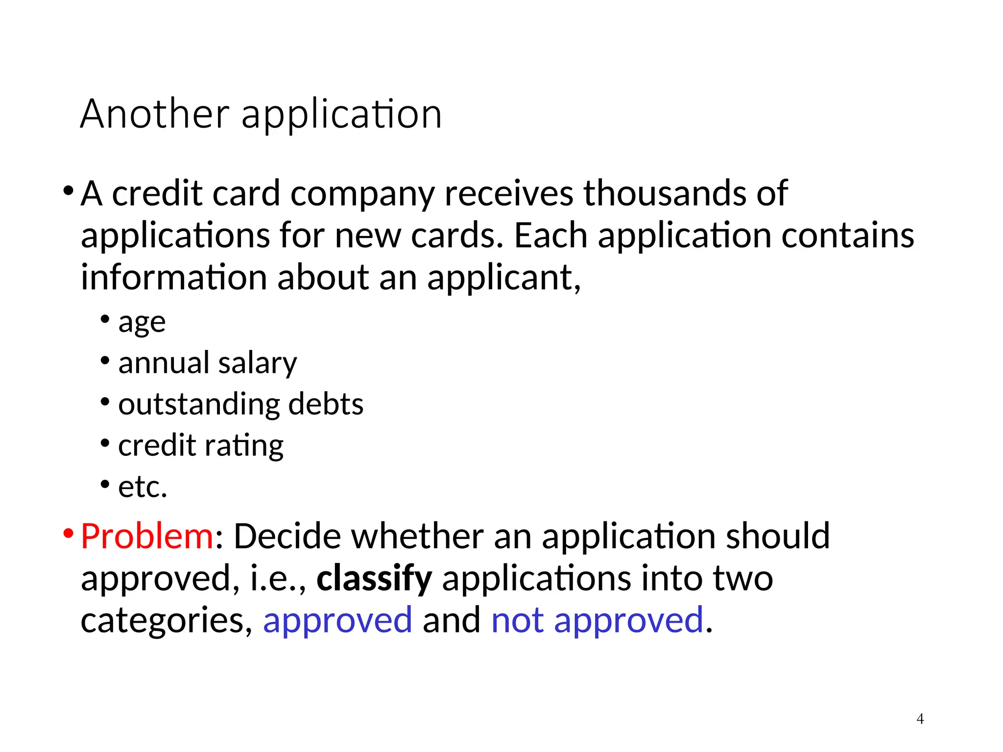
Another application
•A creditcard company receives thousands of
applications for new cards. Each application contains
information about an applicant,
• age
• annual salary
• outstanding debts
• credit rating
• etc.
•Problem: Decide whether an application should
approved, i.e., classify applications into two
categories, approved and not approved.
4
5.
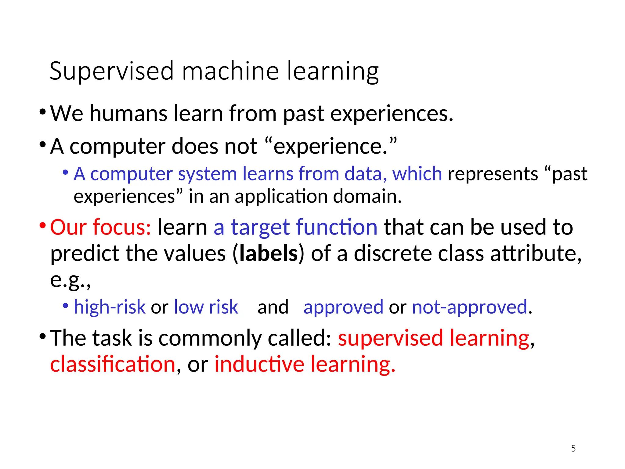
Supervised machine learning
•Wehumans learn from past experiences.
•A computer does not “experience.”
• A computer system learns from data, which represents “past
experiences” in an application domain.
•Our focus: learn a target function that can be used to
predict the values (labels) of a discrete class attribute,
e.g.,
• high-risk or low risk and approved or not-approved.
•The task is commonly called: supervised learning,
classification, or inductive learning.
5
6.
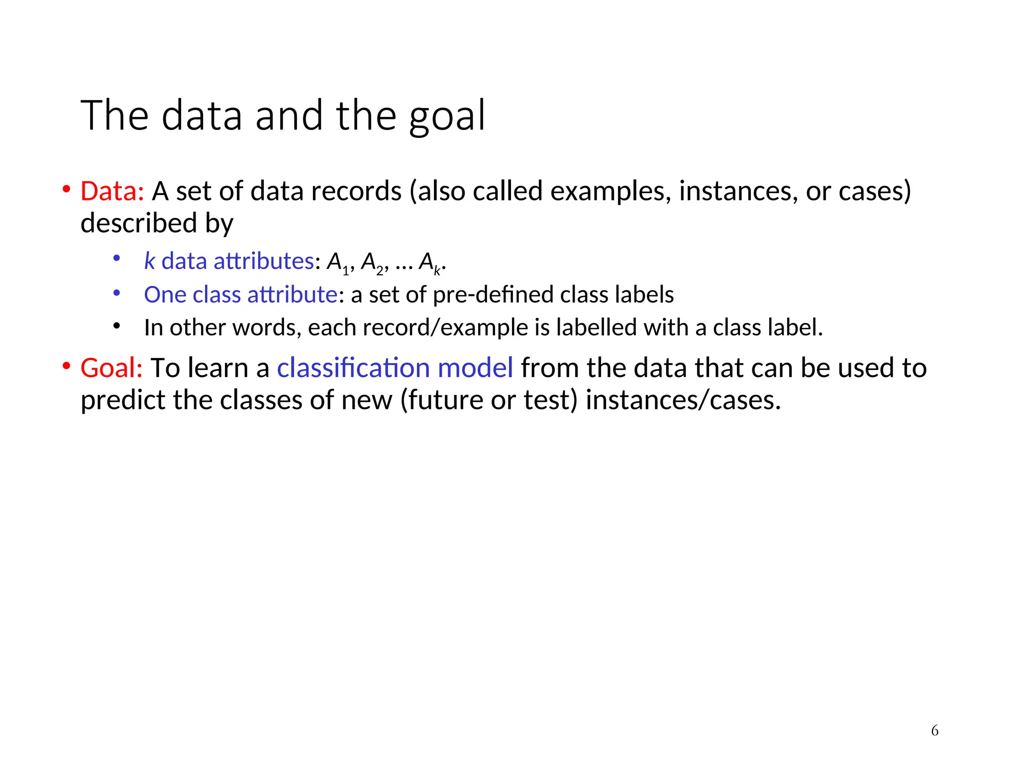
The data andthe goal
• Data: A set of data records (also called examples, instances, or cases)
described by
• k data attributes: A1, A2, … Ak.
• One class attribute: a set of pre-defined class labels
• In other words, each record/example is labelled with a class label.
• Goal: To learn a classification model from the data that can be used to
predict the classes of new (future or test) instances/cases.
6
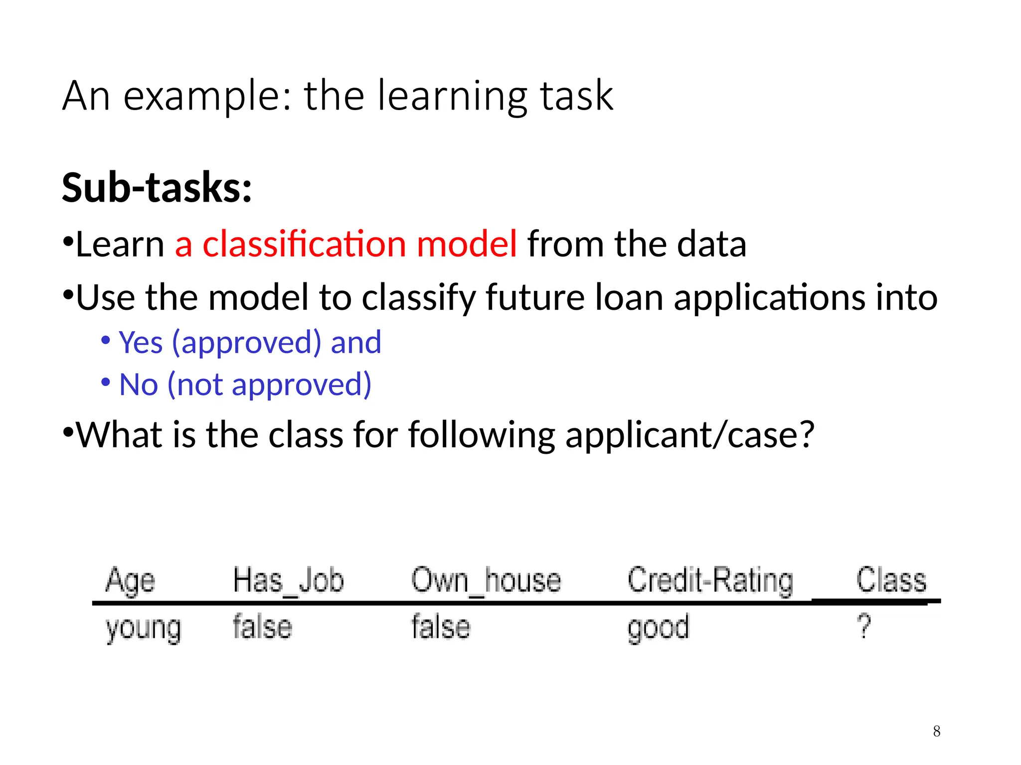
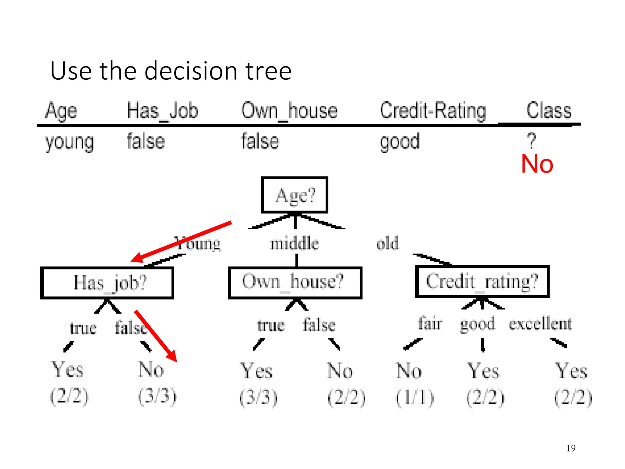
An example: thelearning task
Sub-tasks:
•Learn a classification model from the data
•Use the model to classify future loan applications into
• Yes (approved) and
• No (not approved)
•What is the class for following applicant/case?
8
9.
Supervised vs. unsupervisedLearning
• Supervised learning: classification is supervised learning from examples.
• Supervision: The data (observations, measurements, etc.) are labeled with pre-
defined classes, which is
• like a “teacher” gives us the classes (supervision).
• Unsupervised learning (clustering)
• Class labels of the data are not given or unknown
• Goal: Given a set of data, the task is to establish the existence of classes or clusters in
the data
9
10.
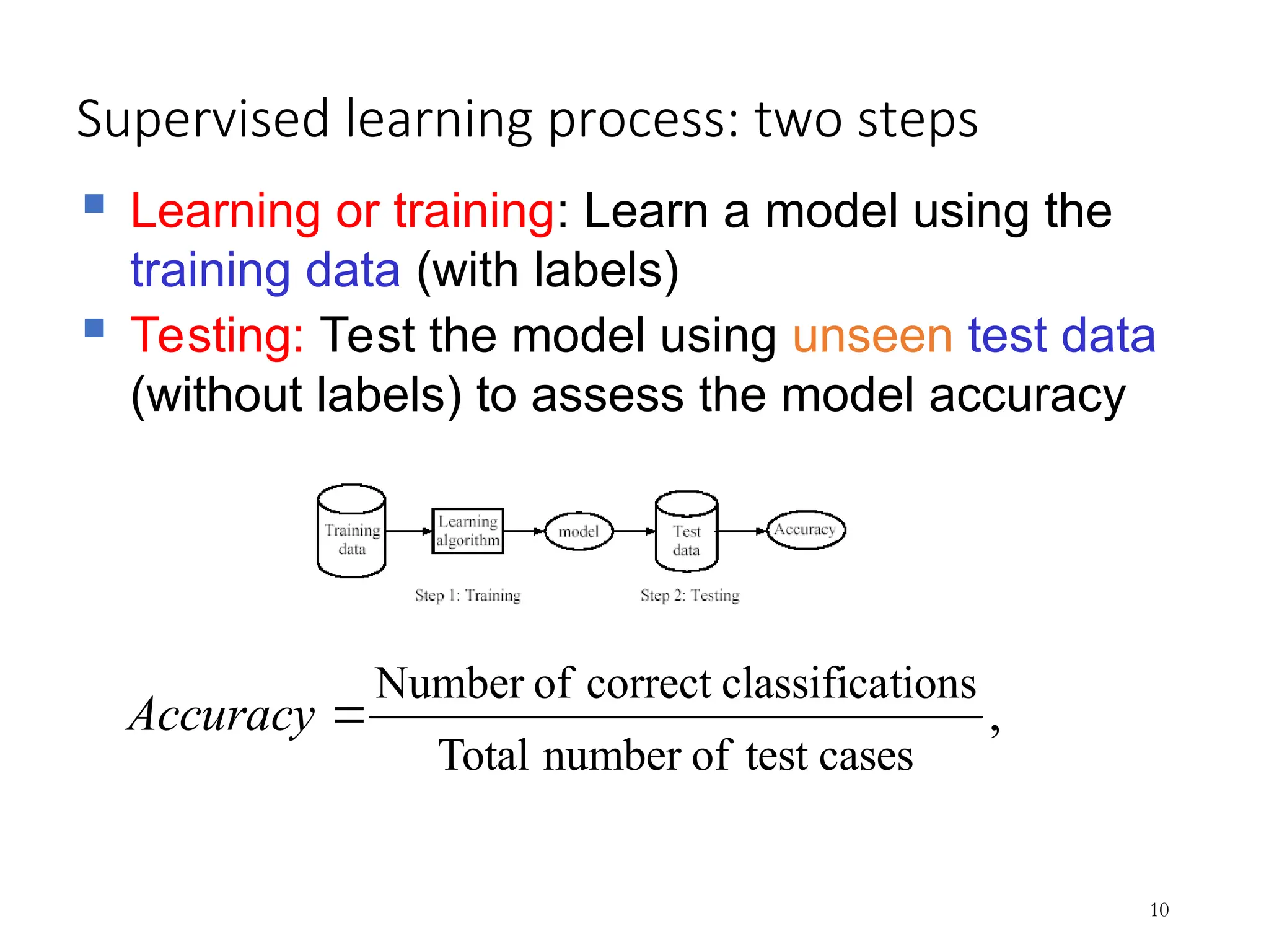
Supervised learning process:two steps
10
Learning or training: Learn a model using the
training data (with labels)
Testing: Test the model using unseen test data
(without labels) to assess the model accuracy
,
cases
test
of
number
Total
tions
classifica
correct
of
Number
Accuracy
11.
What do wemean by learning?
•Given
• a data set D,
• a task T, and
• a performance measure M,
•A computer system is said to learn from D to perform
the task T,
• if after learning, the system’s performance on T improves as
measured by M.
• In other words, the learned model helps the system to
perform T better as compared to without learning.
11
12.
An example
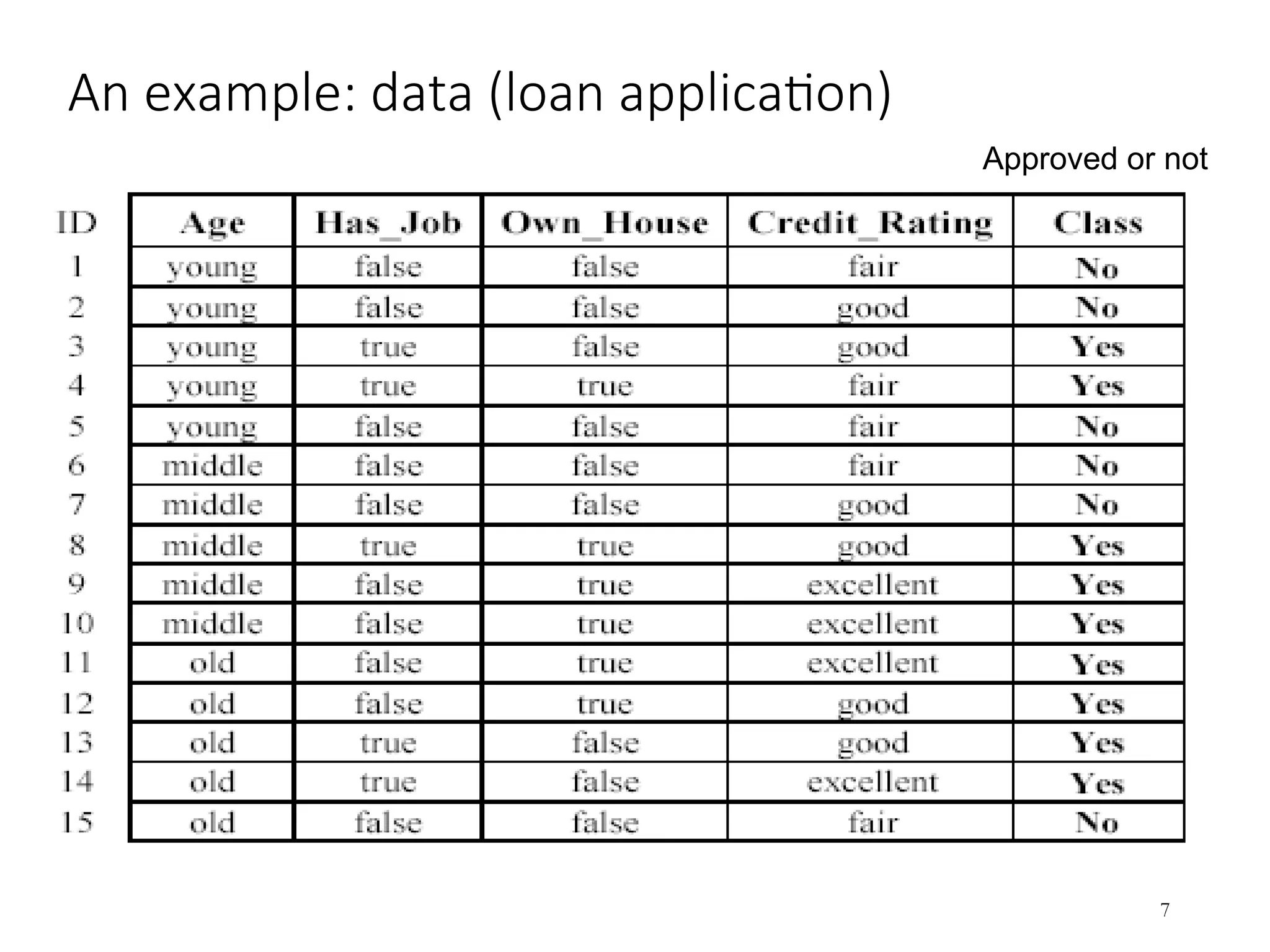
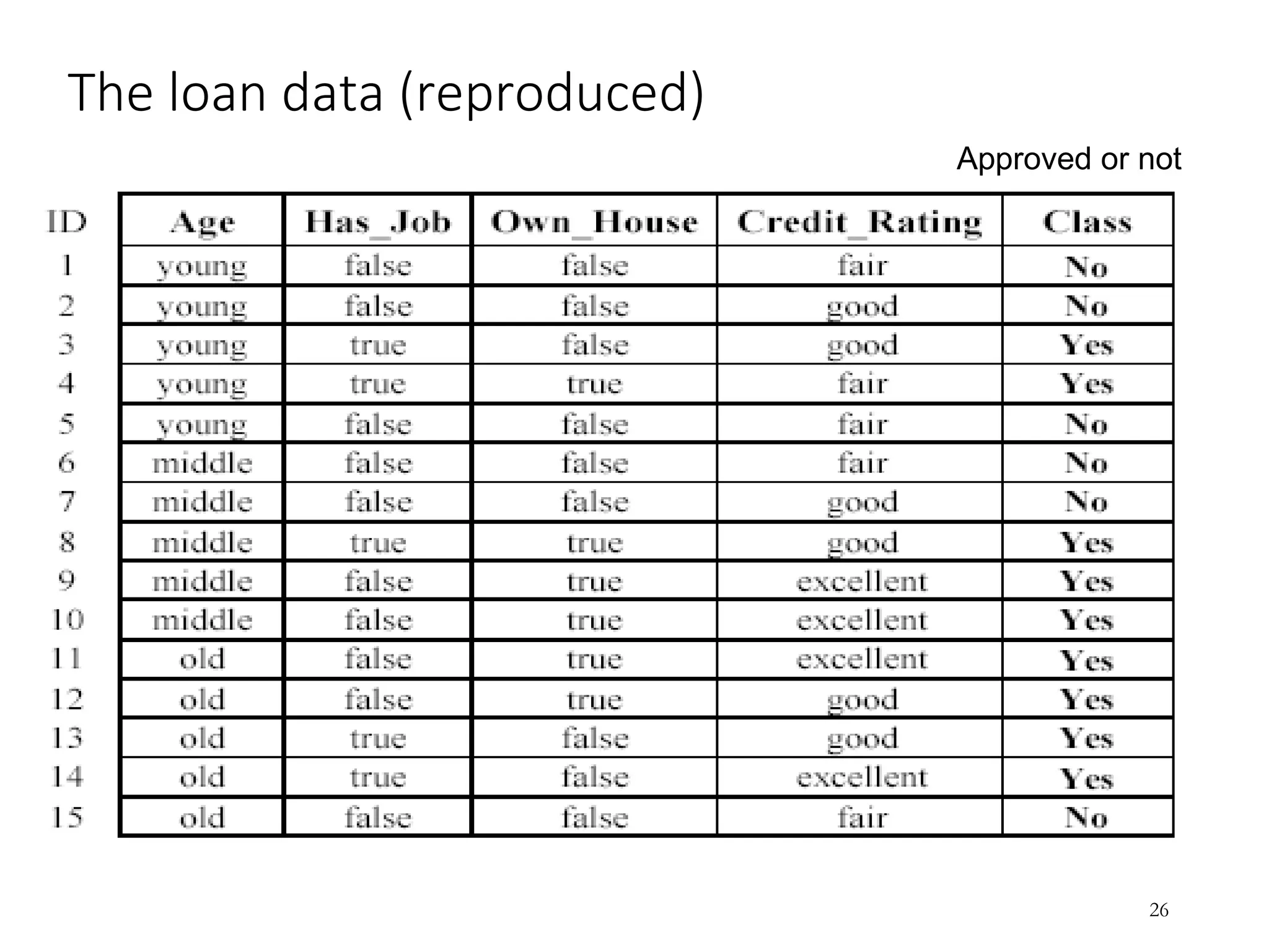
• Data:Loan application data
• Task: Predict whether a loan should be approved or not.
• Performance measure: accuracy.
• No learning: classify all future applications (test data) to the majority
class (i.e., Yes):
Pr(Yes) = 9/15 = 60%.
• Expected accuracy = 60%.
• Can we do better (> 60%) with learning?
12
13.
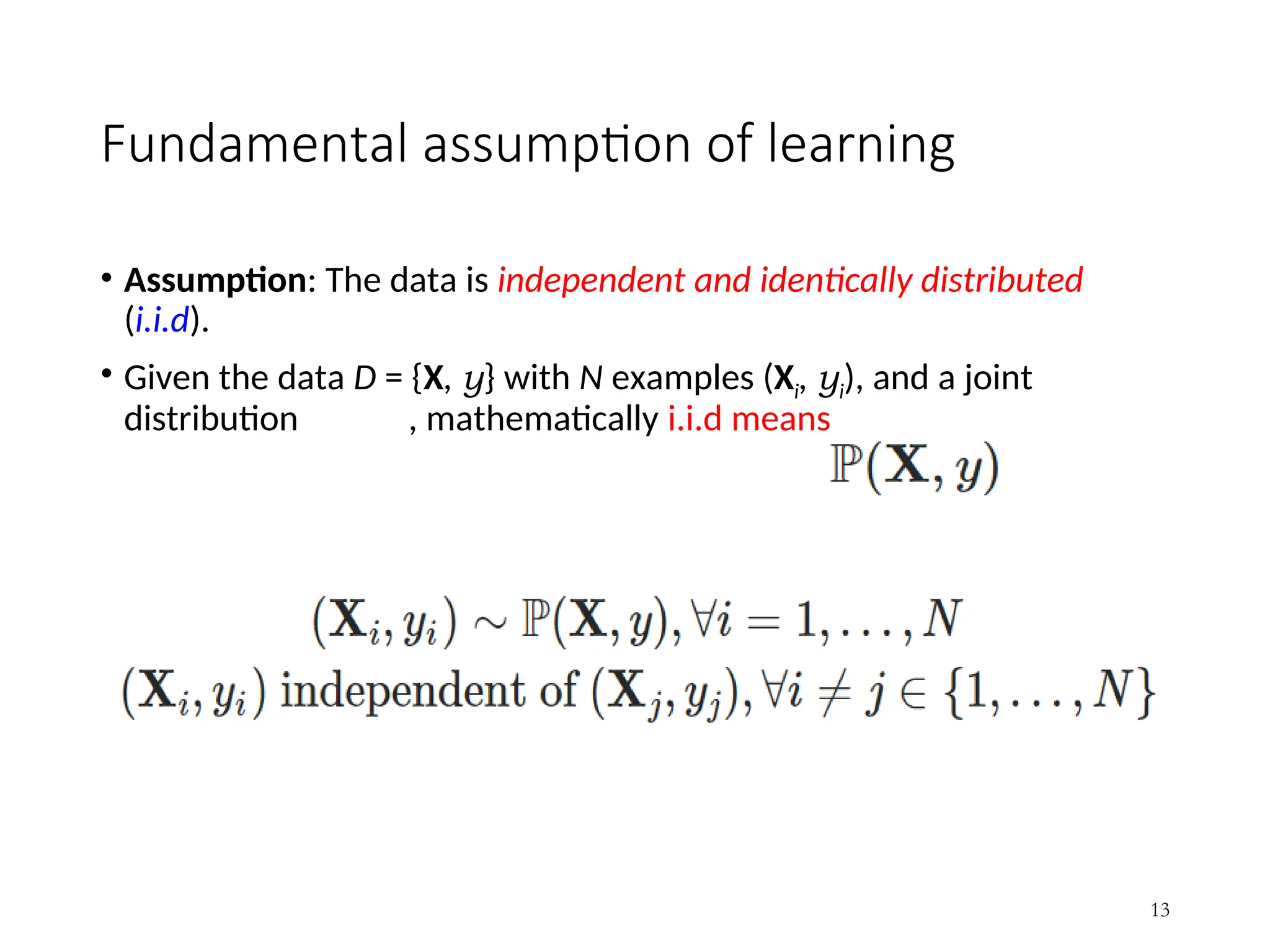
Fundamental assumption oflearning
• Assumption: The data is independent and identically distributed
(i.i.d).
• Given the data D = {X, y} with N examples (Xi, yi), and a joint
distribution , mathematically i.i.d means
13
14.
Fundamental assumption oflearning
• The data is split into training and test data.
• The distribution of training examples is identical to the distribution of test
examples (including future unseen examples).
• To achieve good accuracy on the test data,
• training examples must be sufficiently representative of the test data.
• In practice, this assumption is often violated to certain degree.
• Strong violations will clearly result in poor classification accuracy.
14
15.
Road Map
• Basicconcepts
• Decision tree induction
• Evaluation of classifiers
• Naïve Bayesian classification
• Naïve Bayes for text classification
• Support vector machines
• Linear regression and gradient descent
• Neural networks
• K-nearest neighbor
• Ensemble methods
• Summary
15
16.
Introduction
• Decision treelearning is one of the most widely used techniques for
classification.
• Its accuracy is competitive with other methods,
• it is very efficient.
• The classification model is a tree, called a decision tree.
• C4.5 by Ross Quinlan is perhaps the best known system. It can be
downloaded from the Web.
16
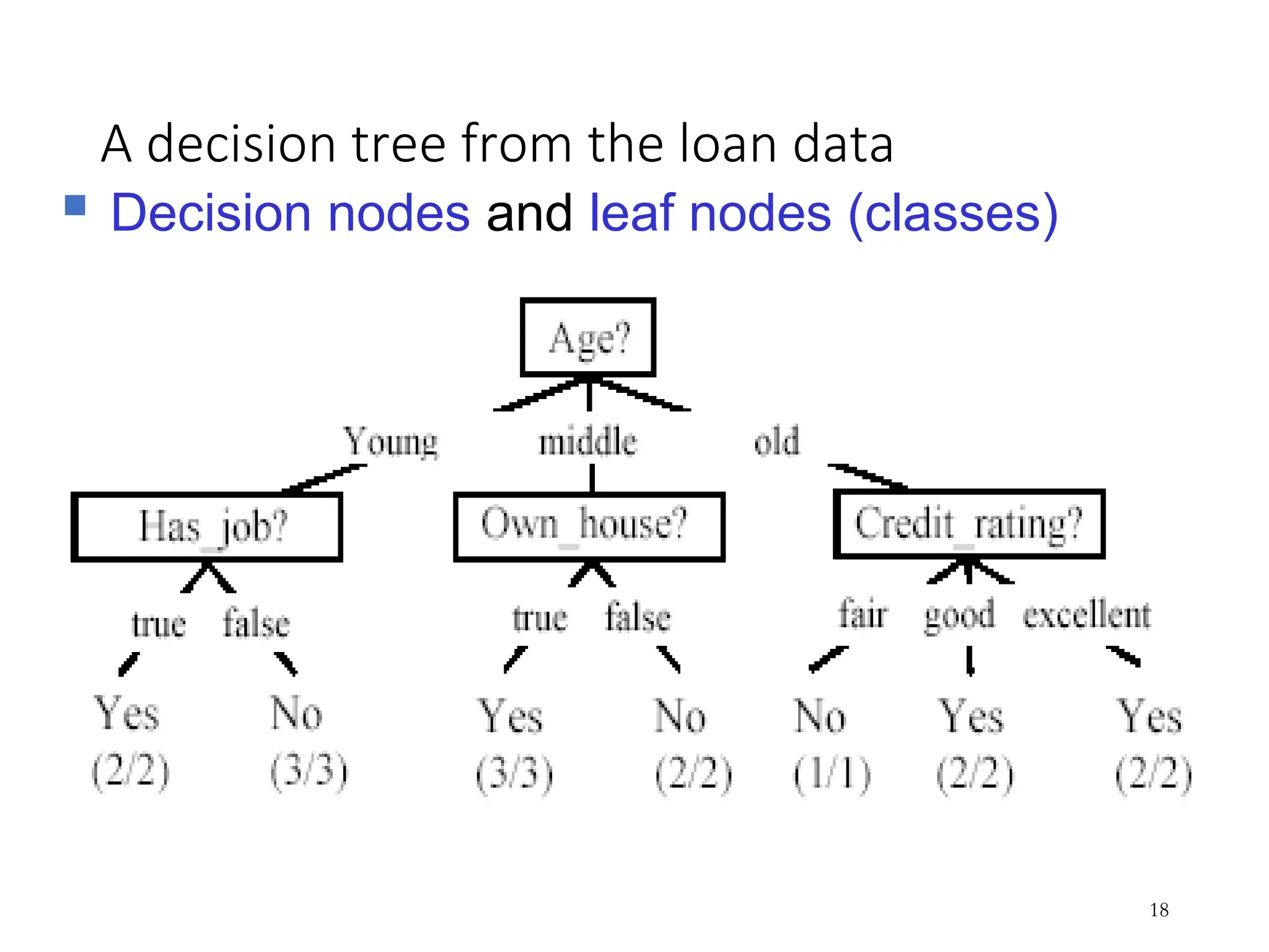
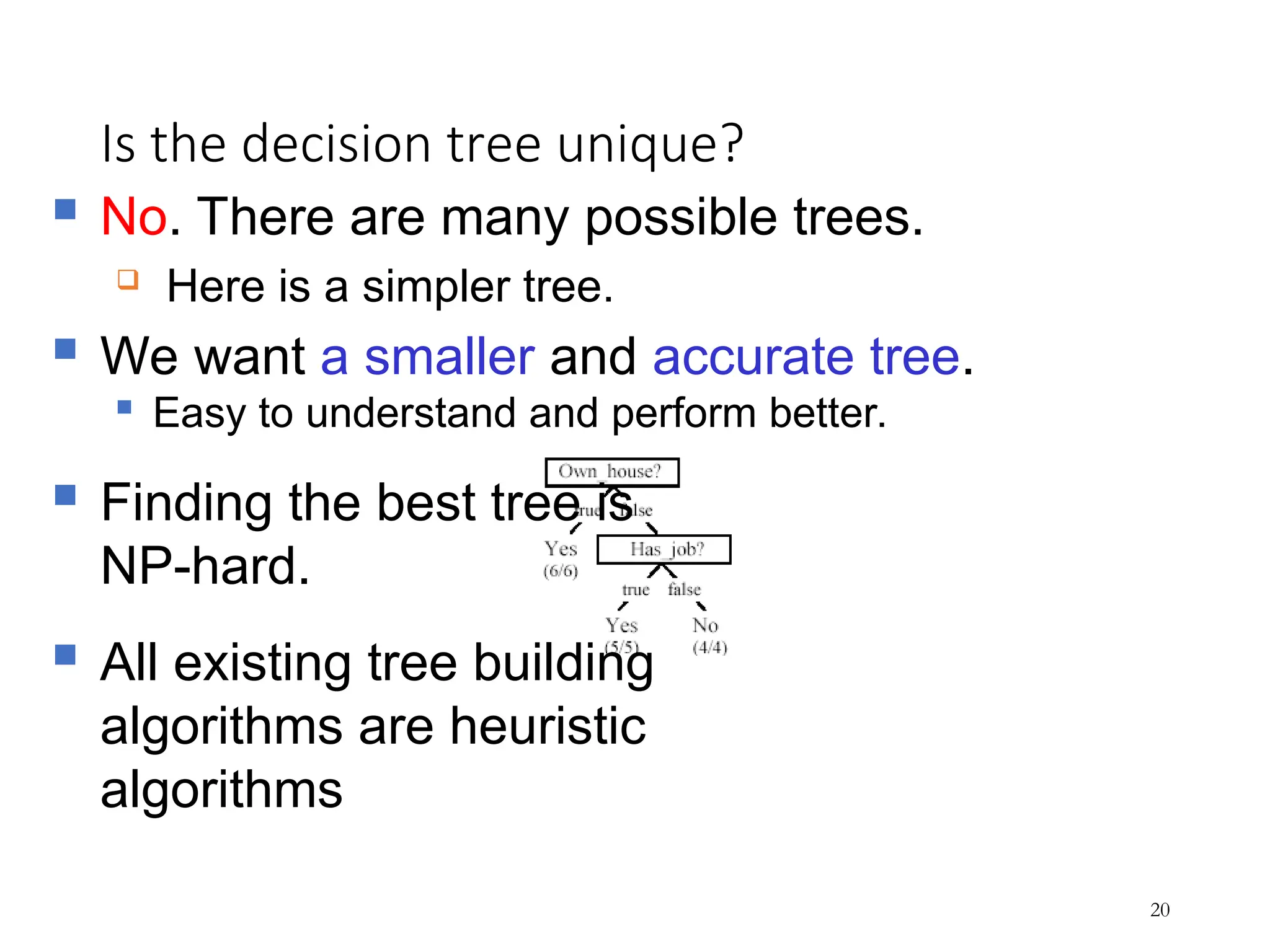
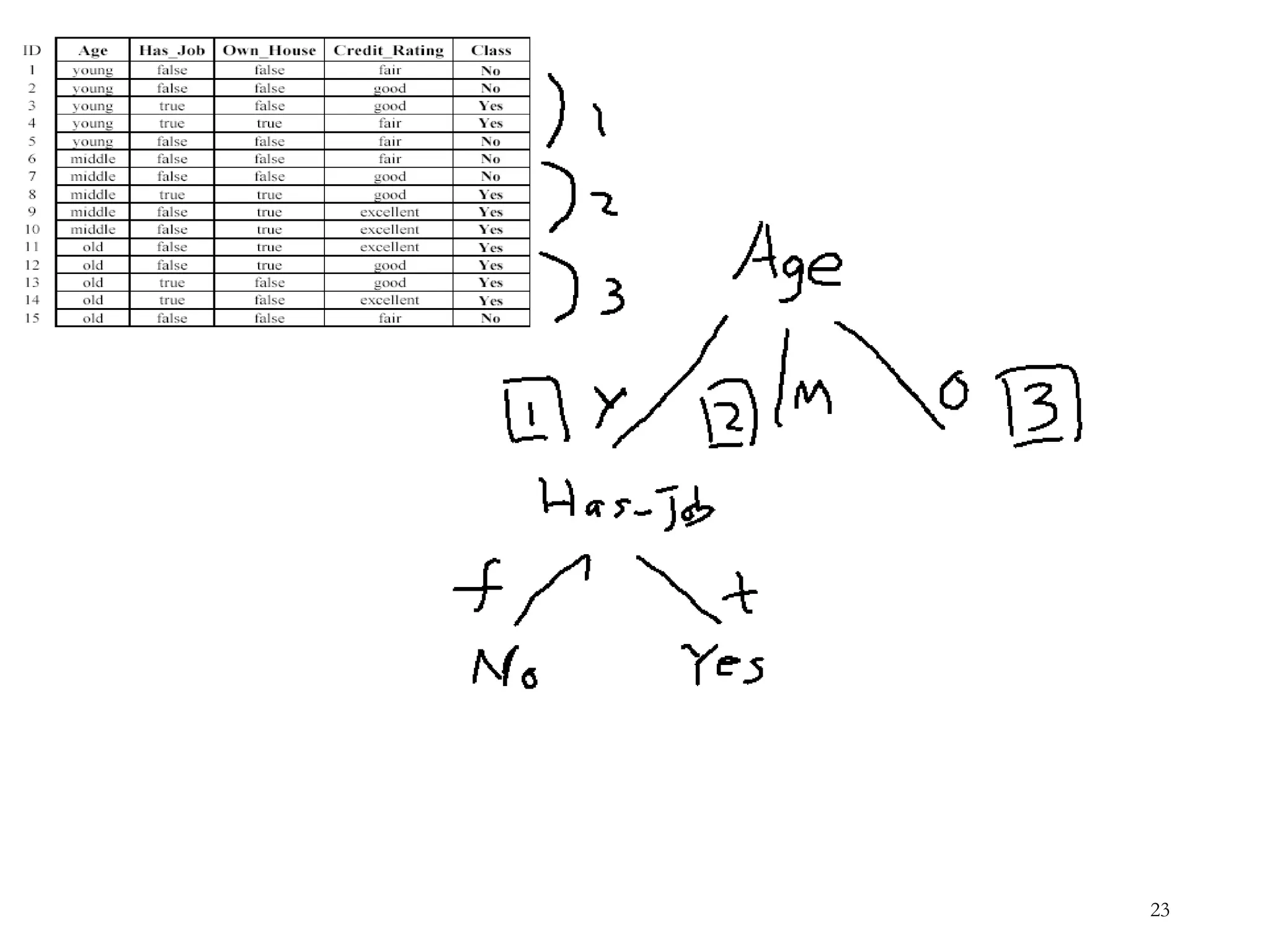
Is the decisiontree unique?
20
No. There are many possible trees.
Here is a simpler tree.
We want a smaller and accurate tree.
Easy to understand and perform better.
Finding the best tree is
NP-hard.
All existing tree building
algorithms are heuristic
algorithms
21.
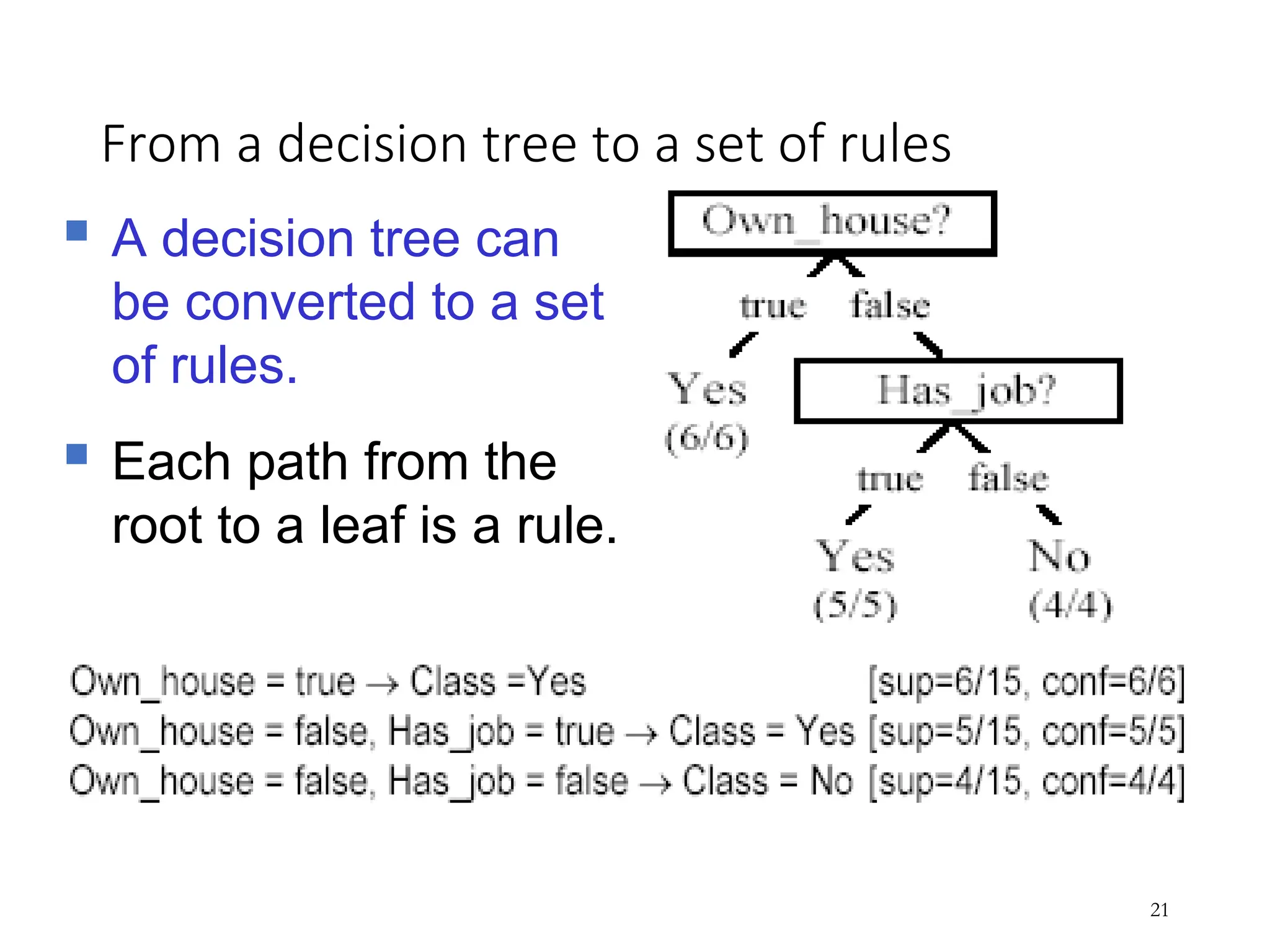
From a decisiontree to a set of rules
21
A decision tree can
be converted to a set
of rules.
Each path from the
root to a leaf is a rule.
22.
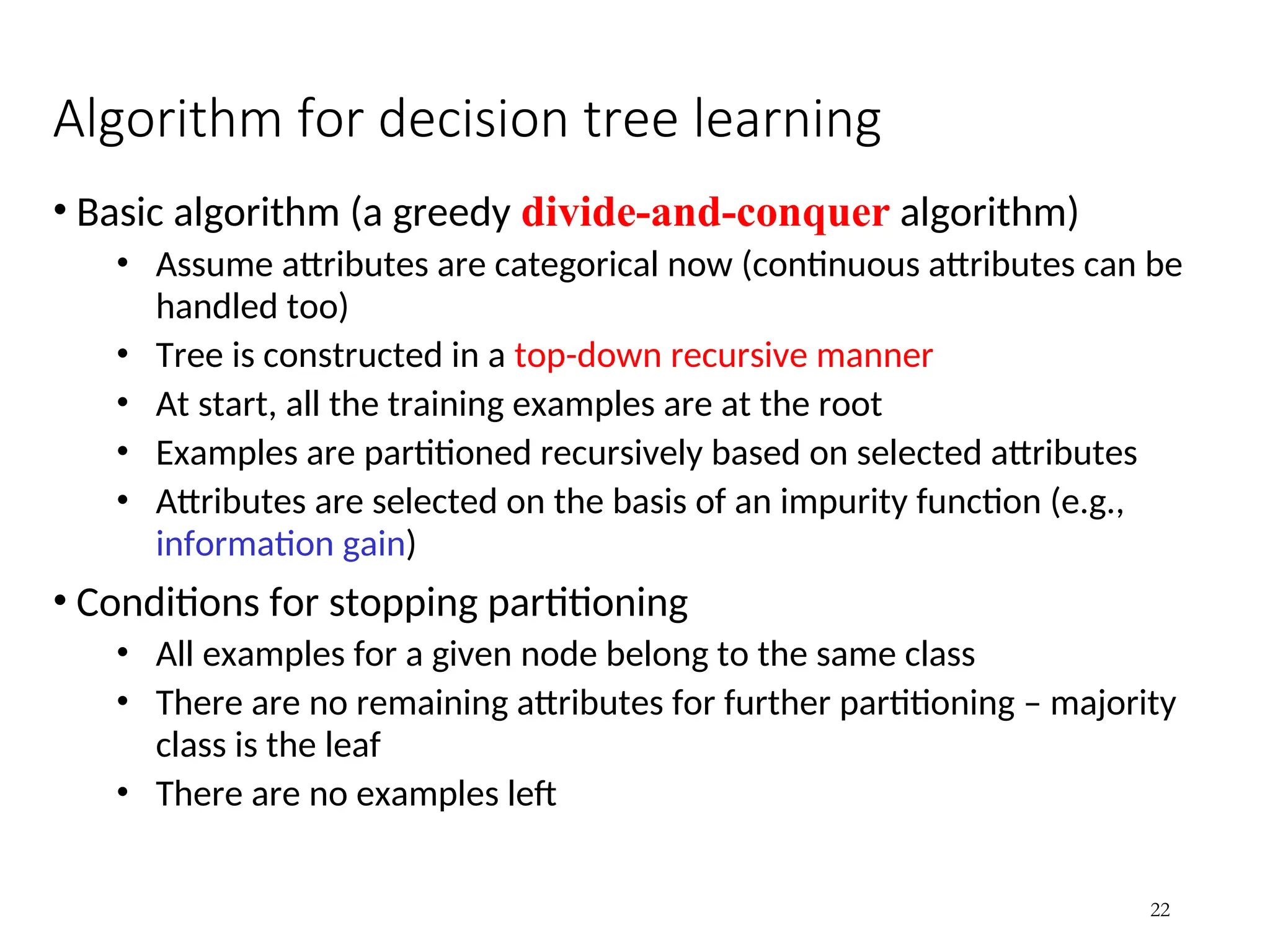
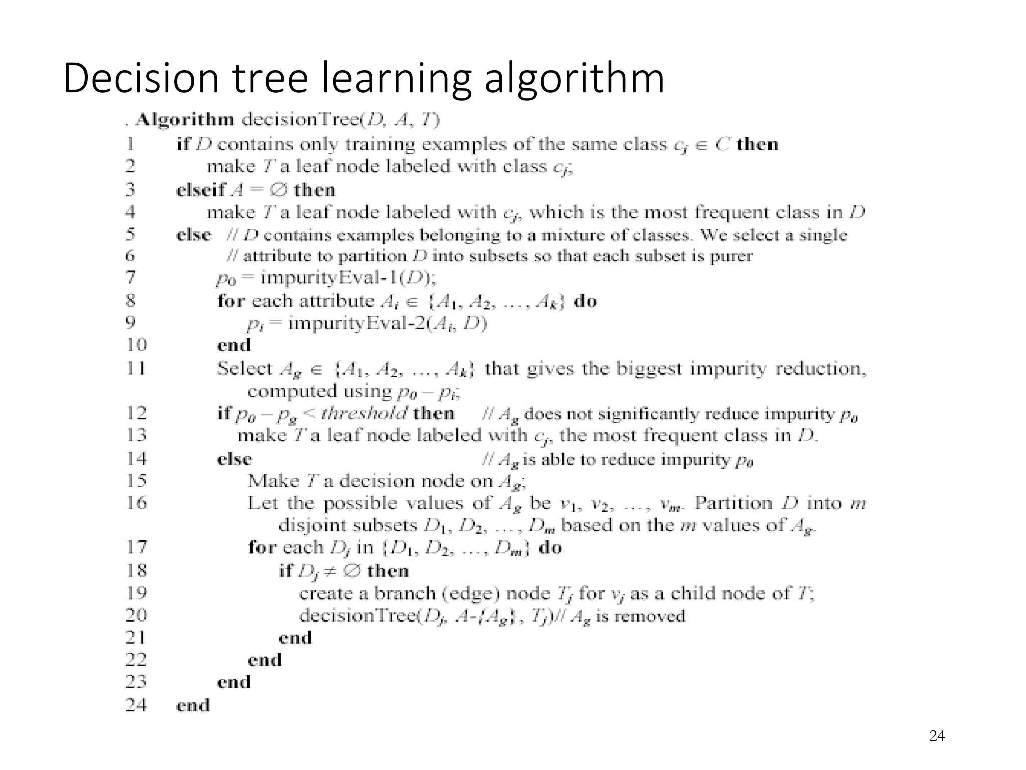
Algorithm for decisiontree learning
• Basic algorithm (a greedy divide-and-conquer algorithm)
• Assume attributes are categorical now (continuous attributes can be
handled too)
• Tree is constructed in a top-down recursive manner
• At start, all the training examples are at the root
• Examples are partitioned recursively based on selected attributes
• Attributes are selected on the basis of an impurity function (e.g.,
information gain)
• Conditions for stopping partitioning
• All examples for a given node belong to the same class
• There are no remaining attributes for further partitioning – majority
class is the leaf
• There are no examples left
22
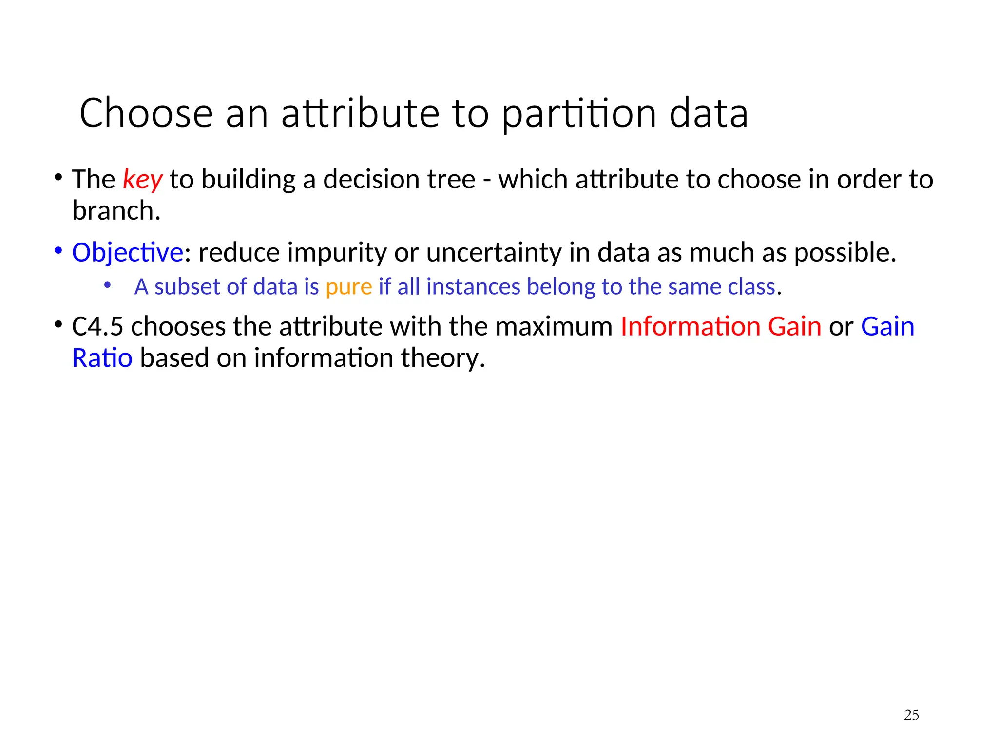
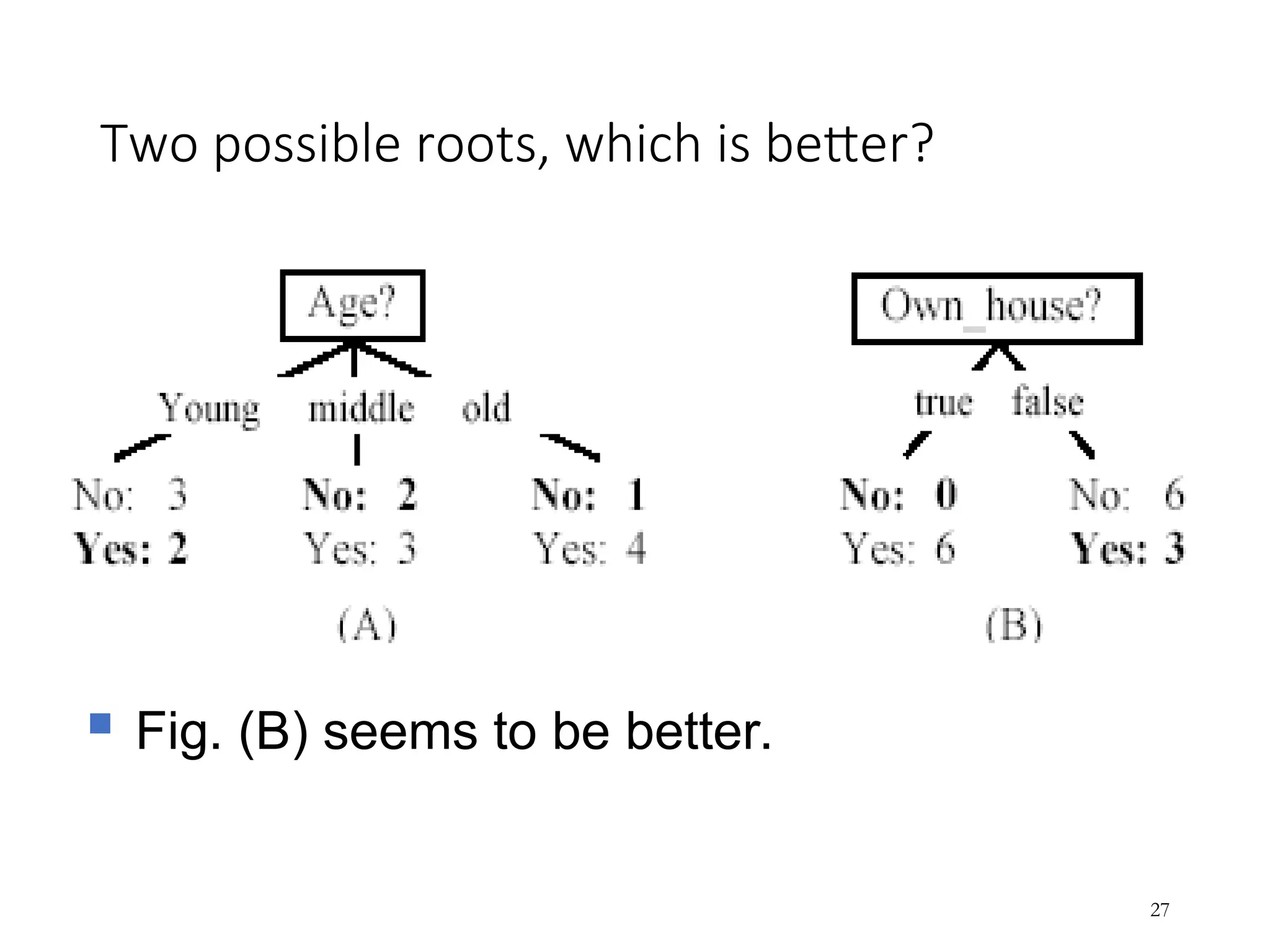
Choose an attributeto partition data
• The key to building a decision tree - which attribute to choose in order to
branch.
• Objective: reduce impurity or uncertainty in data as much as possible.
• A subset of data is pure if all instances belong to the same class.
• C4.5 chooses the attribute with the maximum Information Gain or Gain
Ratio based on information theory.
25
C4.5 uses InformationTheory
•Information theory provides a mathematical basis for
measuring the information content.
•To understand the notion of information, think about
it as providing the answer to a question, e.g., whether
a coin will come up heads.
• If one already has a good guess about the answer, then the
actual answer is less informative.
• If one already knows that the coin is rigged so that it will
come with heads with 0.99 probability, then a message
(advanced information) about the actual outcome of a flip is
worth less than it would be for a honest coin (50-50).
28
29.
Information theory (cont…)
•For a fair (honest) coin,
• you have no information, and you are willing to pay
more (say in terms of $) for advanced information - less
you know, the more valuable the information.
•Information theory uses this same intuition,
• but instead of measuring the value for information in
dollars, it measures information contents in bits.
•One bit of information is enough to answer a
yes/no question about which one has no idea, e.g.,
the flip of a fair coin (50-50).
29
30.
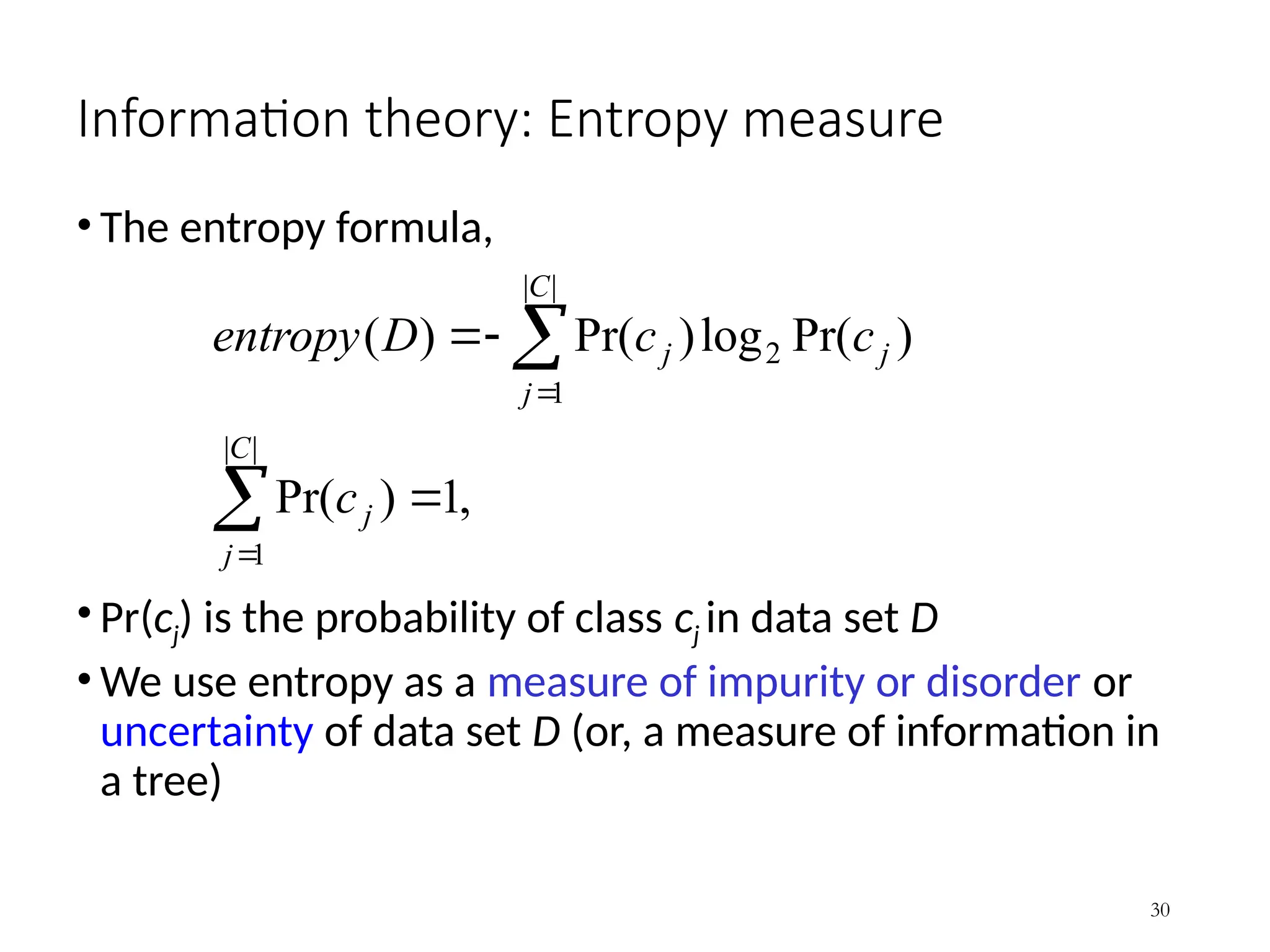
Information theory: Entropymeasure
• The entropy formula,
• Pr(cj) is the probability of class cj in data set D
• We use entropy as a measure of impurity or disorder or
uncertainty of data set D (or, a measure of information in
a tree)
30
,
1
)
Pr(
)
Pr(
log
)
Pr(
)
(
|
|
1
|
|
1
2
C
j
j
j
C
j
j
c
c
c
D
entropy
31.
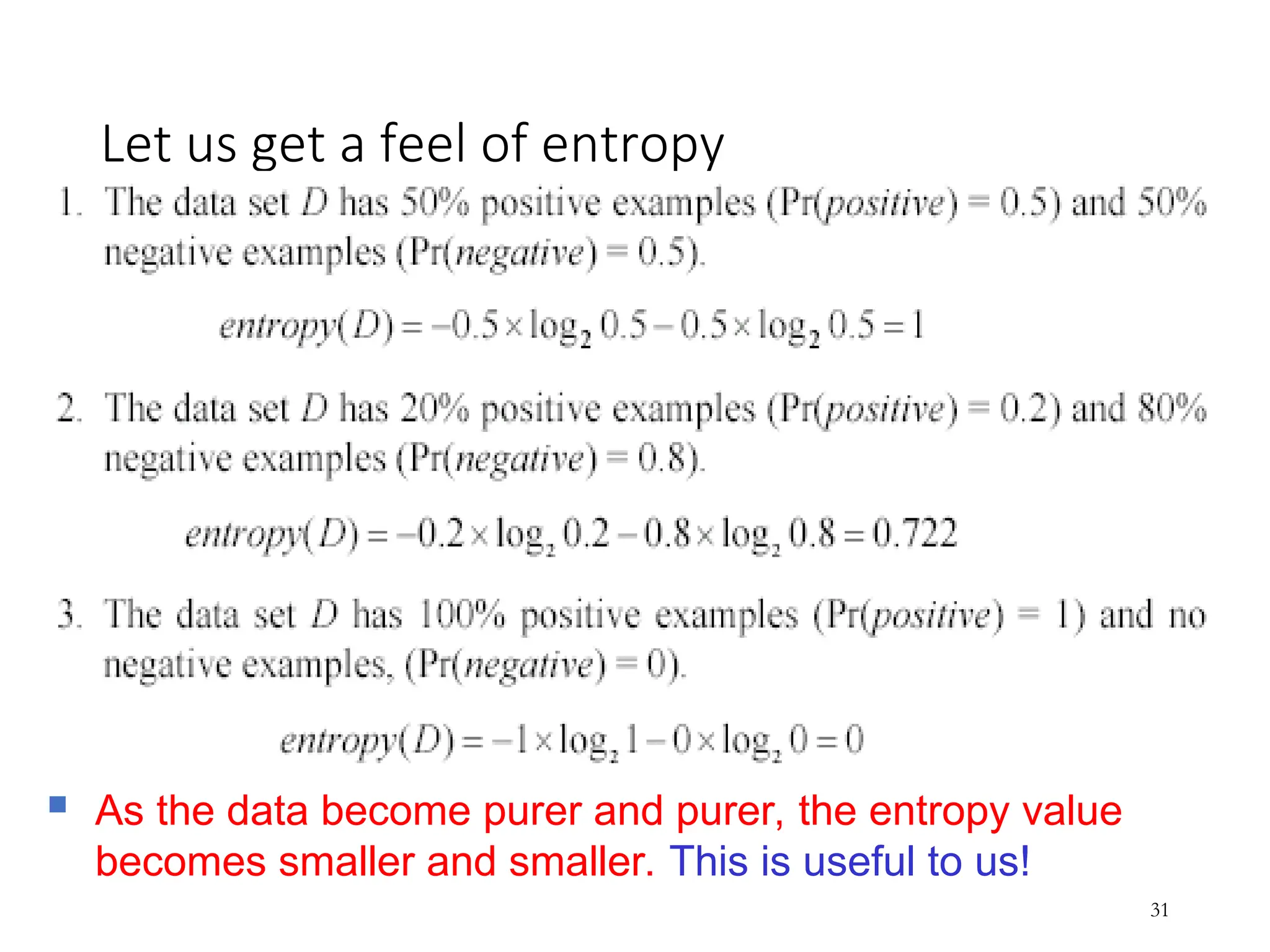
Let us geta feel of entropy
31
As the data become purer and purer, the entropy value
becomes smaller and smaller. This is useful to us!
32.
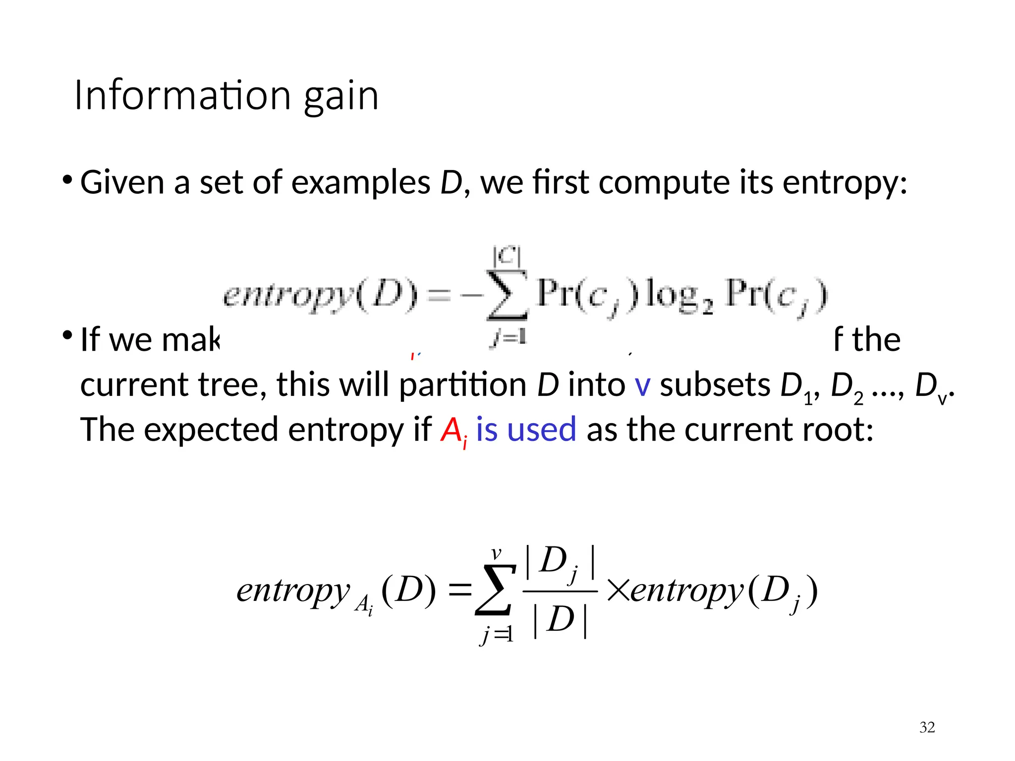
Information gain
• Givena set of examples D, we first compute its entropy:
• If we make attribute Ai, with v values, as the root of the
current tree, this will partition D into v subsets D1, D2 …, Dv.
The expected entropy if Ai is used as the current root:
32
v
j
j
j
A D
entropy
D
D
D
entropy i
1
)
(
|
|
|
|
)
(
33.
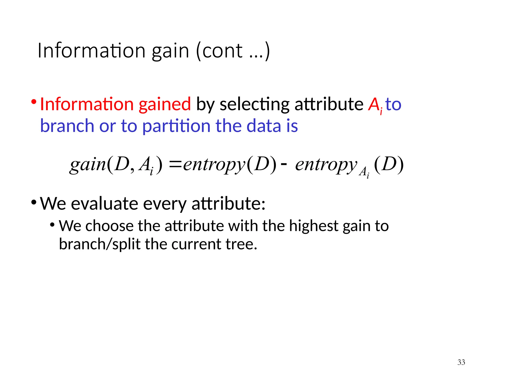
Information gain (cont…)
•Information gained by selecting attribute Ai to
branch or to partition the data is
•We evaluate every attribute:
• We choose the attribute with the highest gain to
branch/split the current tree.
33
)
(
)
(
)
,
( D
entropy
D
entropy
A
D
gain i
A
i
34.
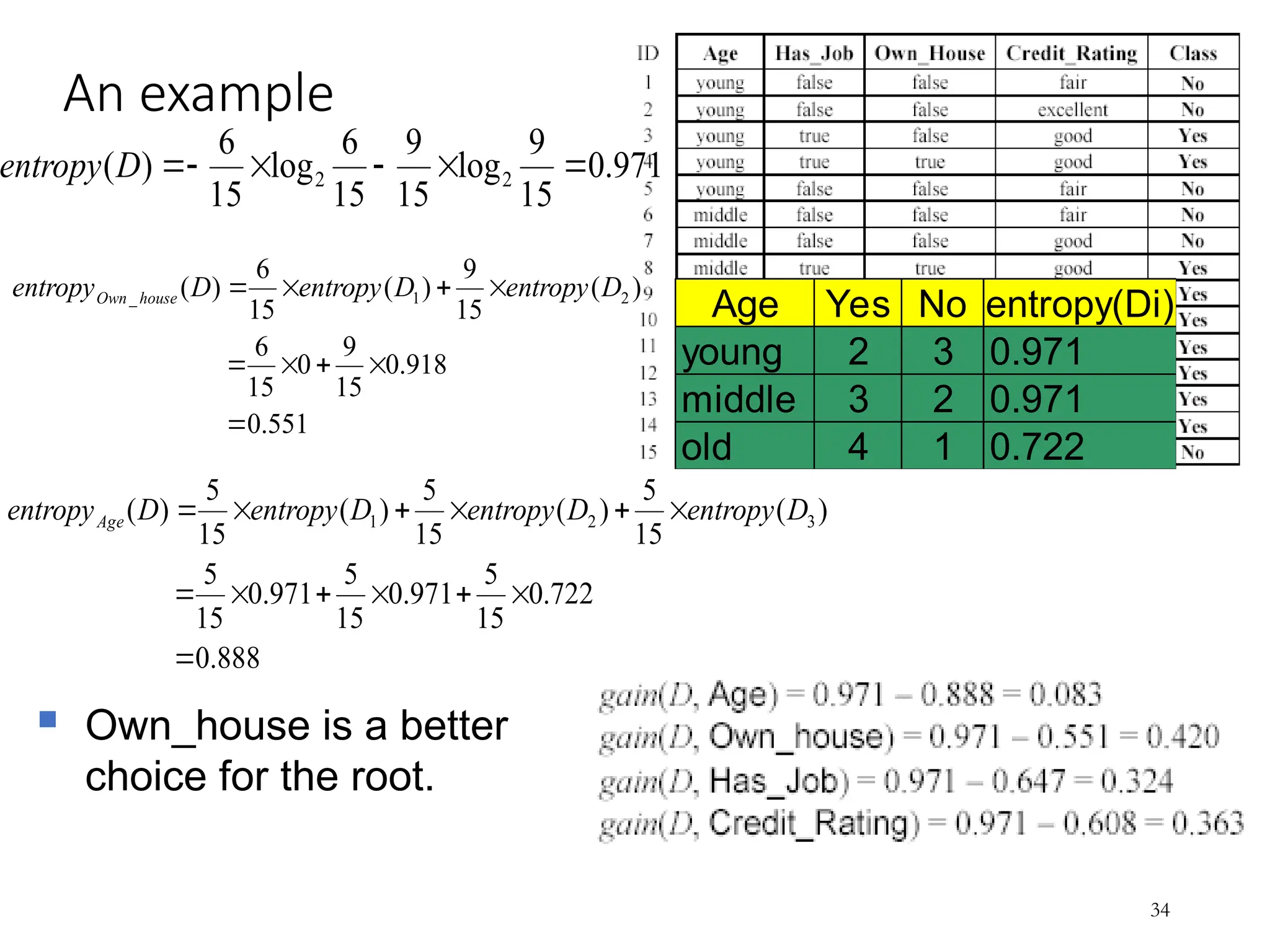
An example
Age YesNo entropy(Di)
young 2 3 0.971
middle 3 2 0.971
old 4 1 0.722
34
Own_house is a better
choice for the root.
971
.
0
15
9
log
15
9
15
6
log
15
6
)
( 2
2
D
entropy
551
.
0
918
.
0
15
9
0
15
6
)
(
15
9
)
(
15
6
)
( 2
1
_
D
entropy
D
entropy
D
entropy house
Own
888
.
0
722
.
0
15
5
971
.
0
15
5
971
.
0
15
5
)
(
15
5
)
(
15
5
)
(
15
5
)
( 3
2
1
D
entropy
D
entropy
D
entropy
D
entropyAge
35.
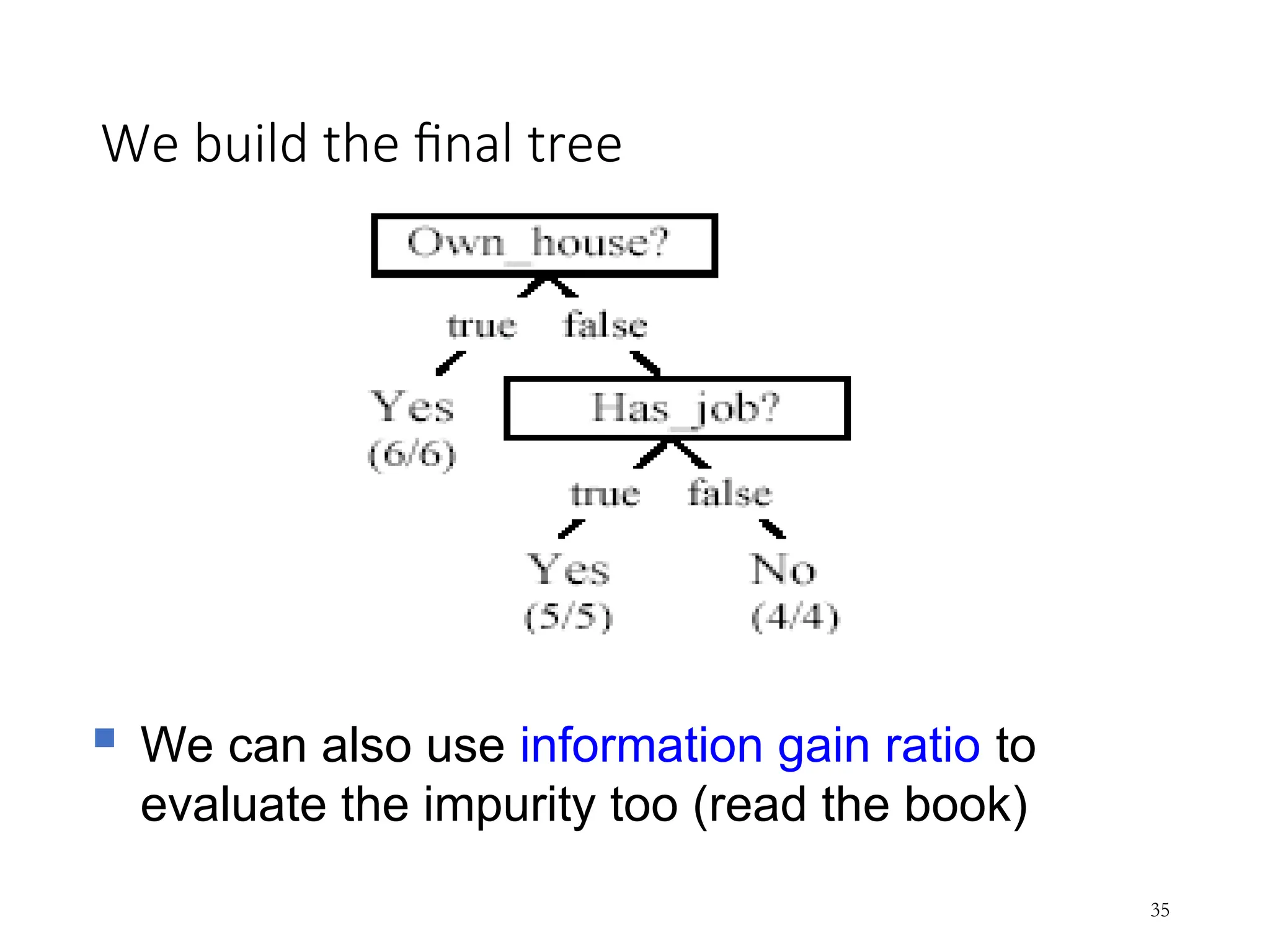
We build thefinal tree
35
We can also use information gain ratio to
evaluate the impurity too (read the book)
36.
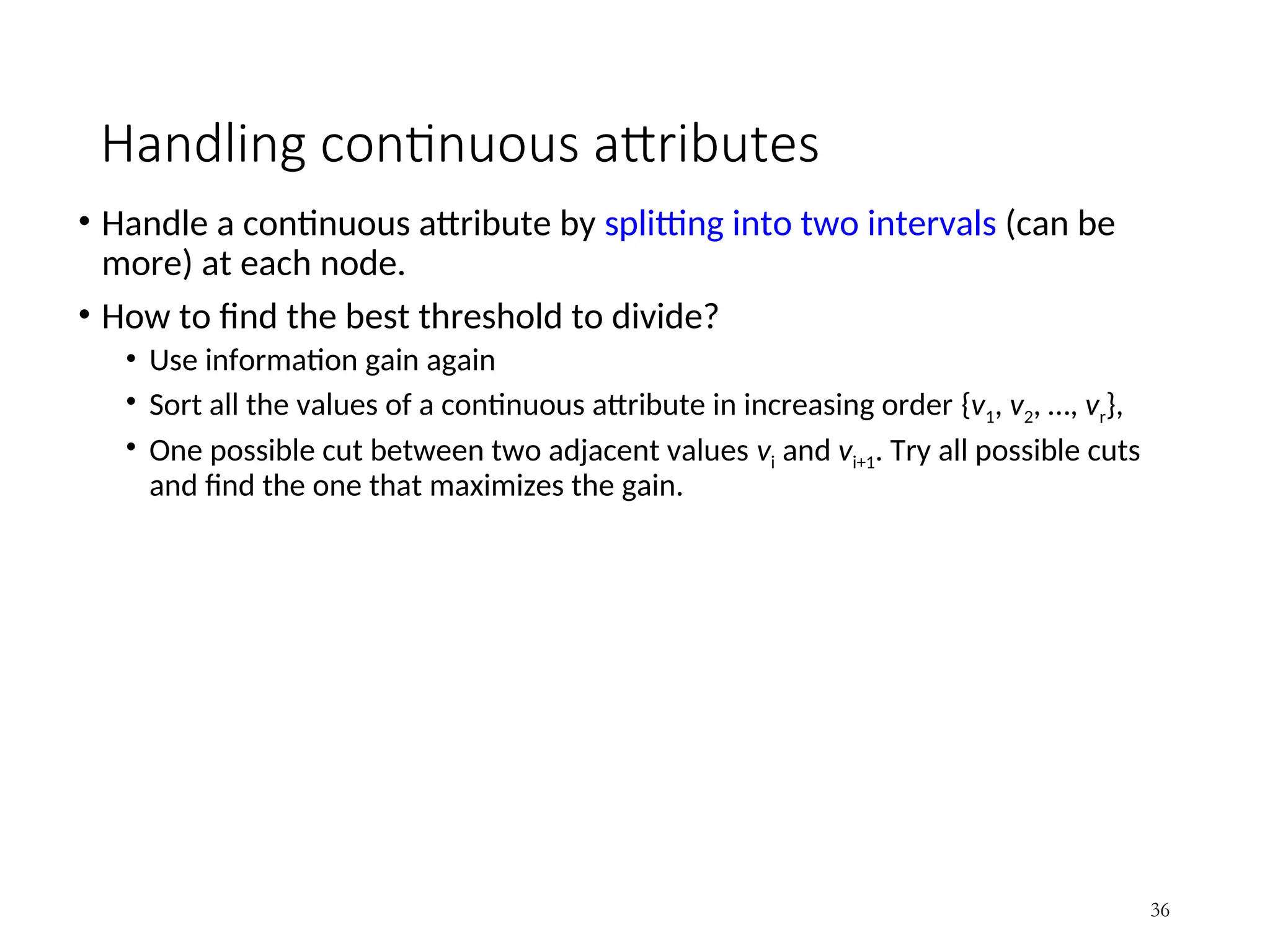
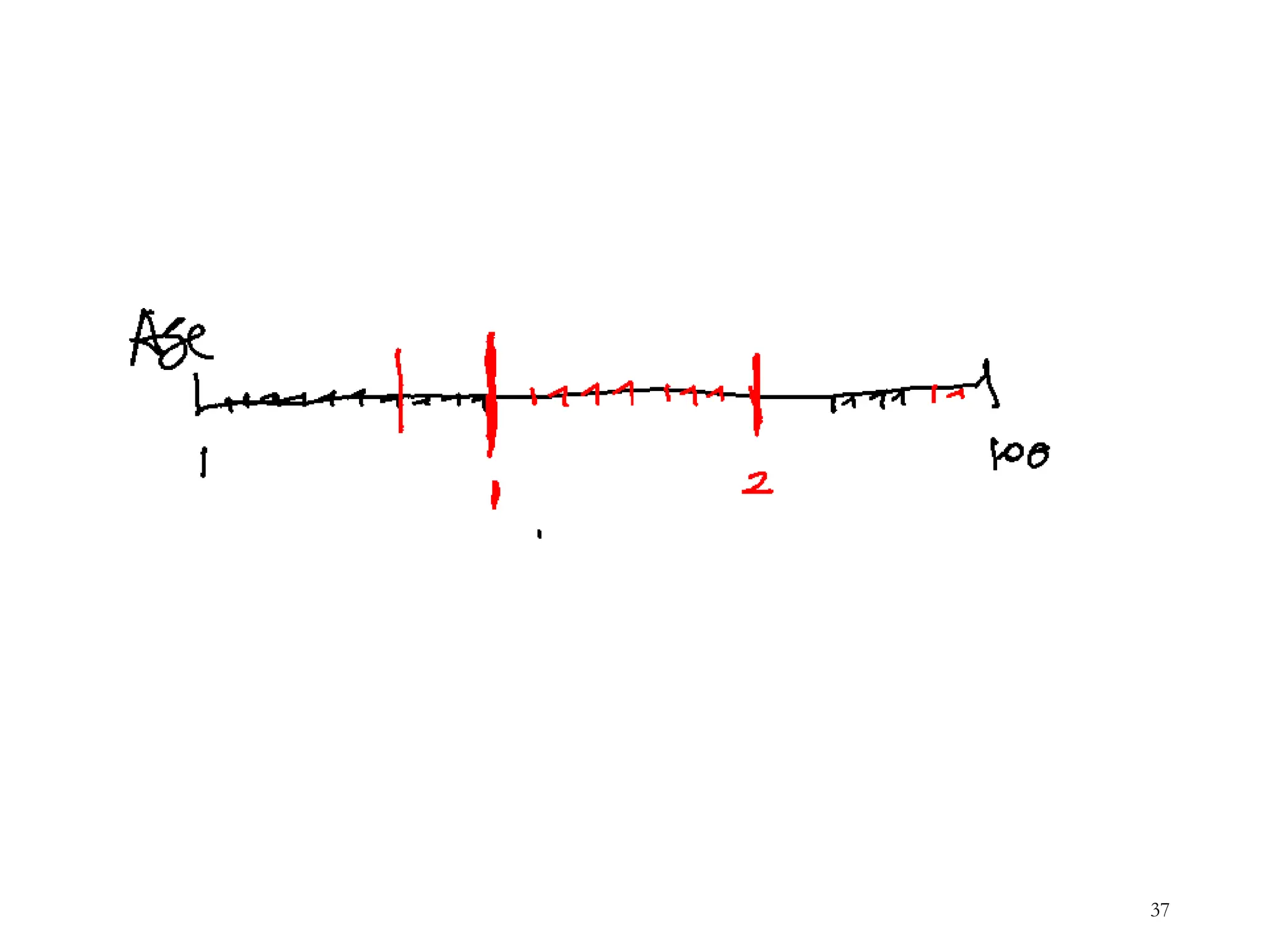
Handling continuous attributes
•Handle a continuous attribute by splitting into two intervals (can be
more) at each node.
• How to find the best threshold to divide?
• Use information gain again
• Sort all the values of a continuous attribute in increasing order {v1, v2, …, vr},
• One possible cut between two adjacent values vi and vi+1. Try all possible cuts
and find the one that maximizes the gain.
36
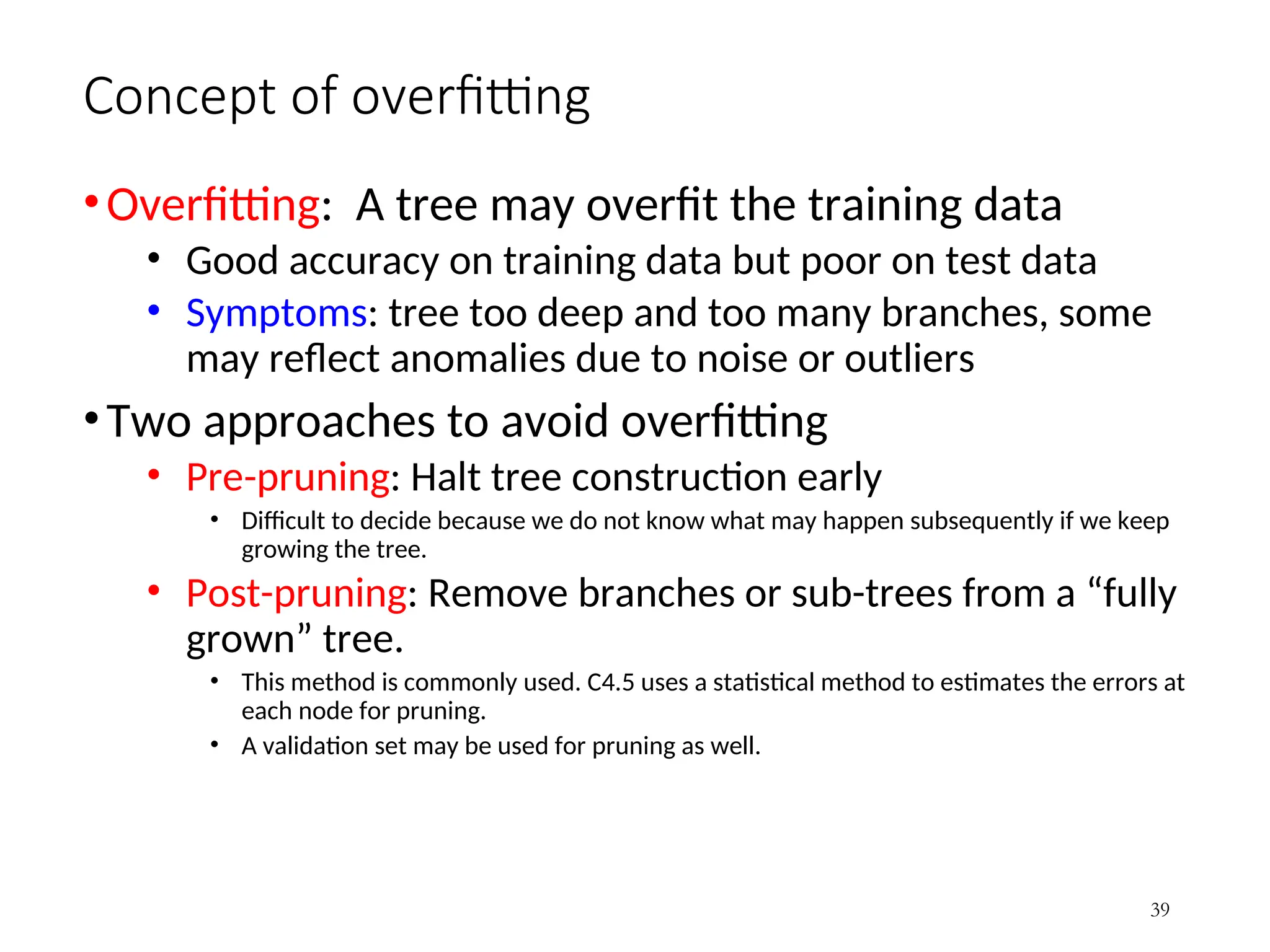
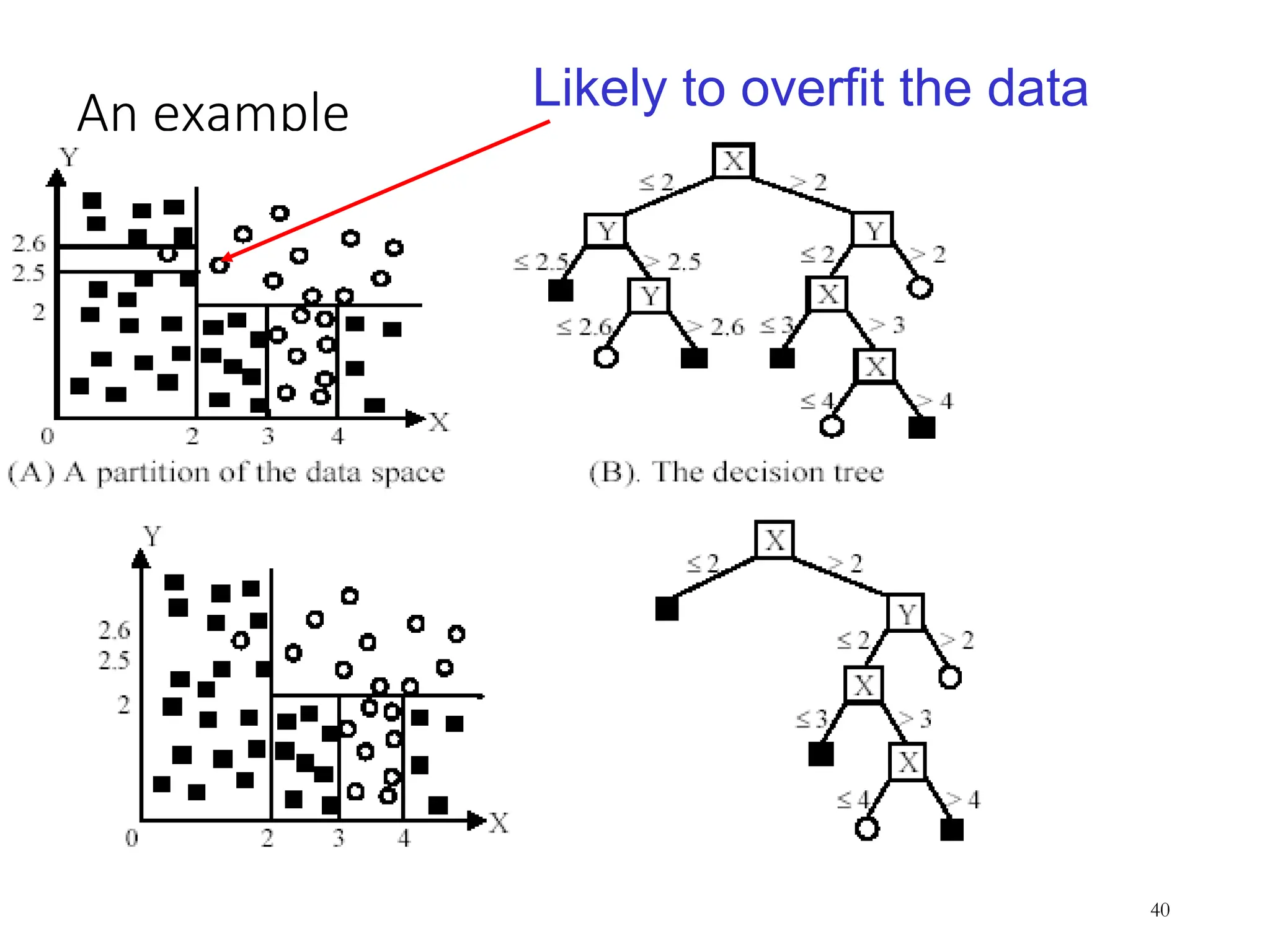
Concept of overfitting
•Overfitting:A tree may overfit the training data
• Good accuracy on training data but poor on test data
• Symptoms: tree too deep and too many branches, some
may reflect anomalies due to noise or outliers
•Two approaches to avoid overfitting
• Pre-pruning: Halt tree construction early
• Difficult to decide because we do not know what may happen subsequently if we keep
growing the tree.
• Post-pruning: Remove branches or sub-trees from a “fully
grown” tree.
• This method is commonly used. C4.5 uses a statistical method to estimates the errors at
each node for pruning.
• A validation set may be used for pruning as well.
39
Other issues indecision tree learning
• From tree to rules, and rule pruning
• Handling of miss values
• Handing skewed distributions
• Handling attributes and classes with different costs.
• Attribute construction
• Etc.
41
42.
Road Map
• Basicconcepts
• Decision tree induction
• Evaluation of classifiers
• Naïve Bayesian classification
• Naïve Bayes for text classification
• Support vector machines
• Linear regression and gradient descent
• Neural networks
• K-nearest neighbor
• Ensemble methods
• Summary
42
43.
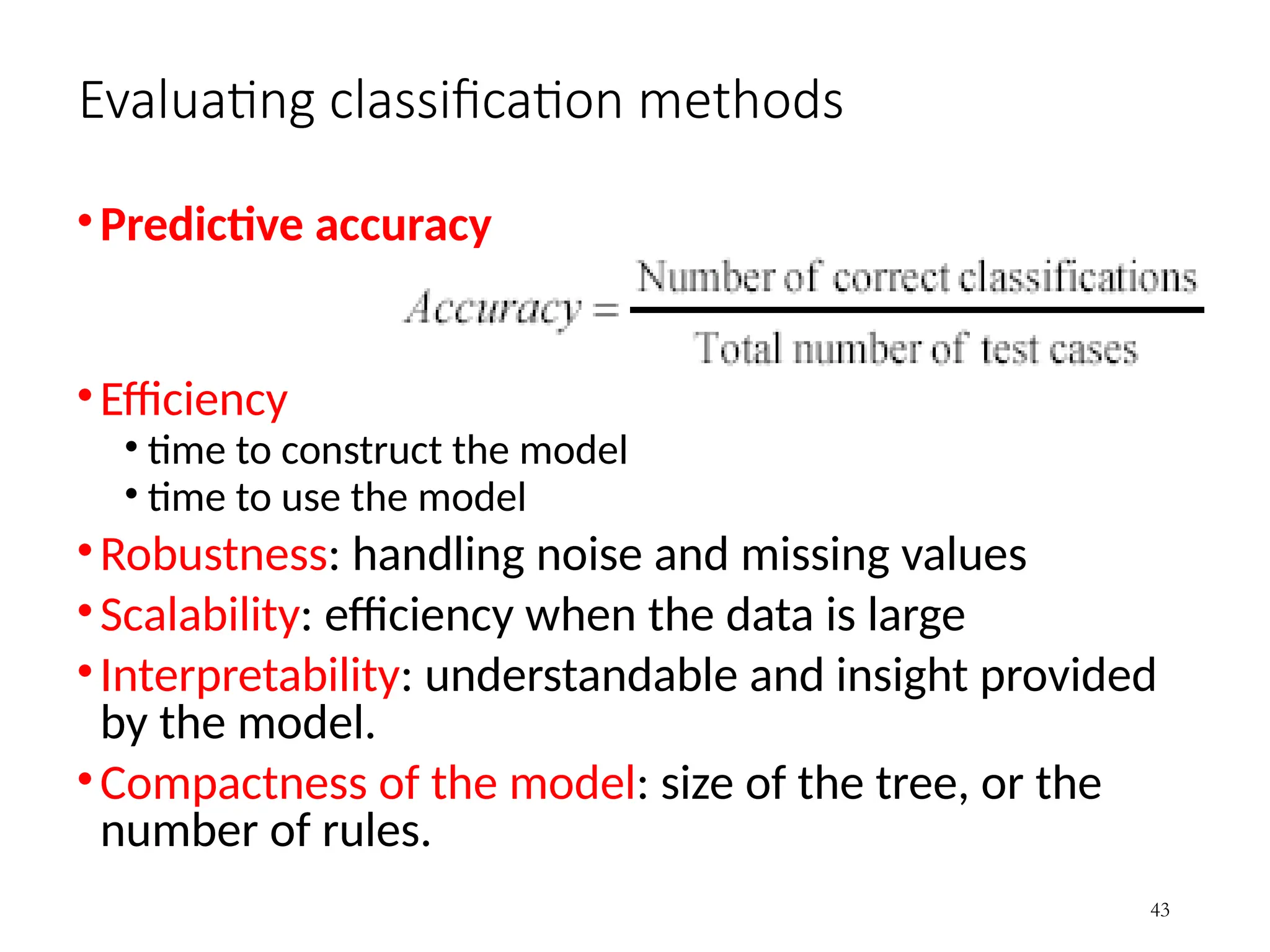
Evaluating classification methods
•Predictiveaccuracy
•Efficiency
• time to construct the model
• time to use the model
•Robustness: handling noise and missing values
•Scalability: efficiency when the data is large
•Interpretability: understandable and insight provided
by the model.
•Compactness of the model: size of the tree, or the
number of rules.
43
44.
Evaluation methods
• Holdoutset: The available data set D is divided into two
disjoint subsets,
• the training set Dtrain (for learning a model)
• the test set Dtest (for testing the model)
• Important: training set should not be used in testing and
the test set should not be used in learning.
• Unseen test set provides a unbiased estimate of accuracy.
• The test set is also called the holdout set. (the examples in
the original data set D are all labeled with classes.)
• This method is used when the data set D is large.
44
45.
Evaluation methods (cont…)
•n-foldcross-validation: The available data is partitioned
into n equal-size disjoint subsets.
•Use each subset as the test set and combine the rest n-
1 subsets as the training set to learn a classifier.
• The procedure is run n times, which give n accuracies.
•The final estimated accuracy of learning is the average
of the n accuracies.
•10-fold and 5-fold cross-validations are commonly used.
45
46.
Evaluation methods (cont…)
•Leave-one-out cross-validation:
• used when the data set is very small.
• a special case of cross-validation
• Each fold of the cross validation has only a single test example and all
the rest of the data is used in training.
• If the original data has m examples, this is m-fold cross-validation
46
47.
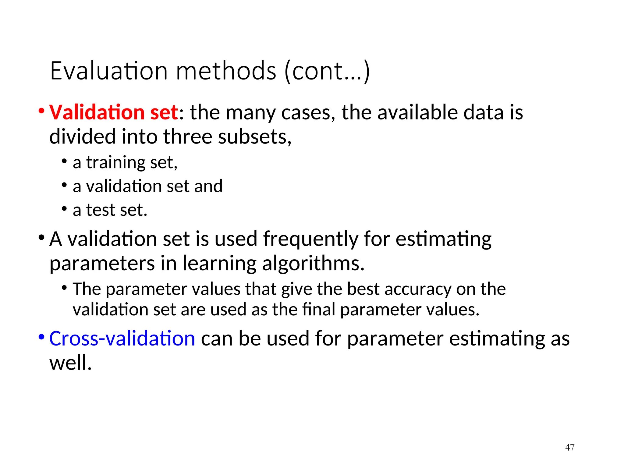
Evaluation methods (cont…)
•Validation set: the many cases, the available data is
divided into three subsets,
• a training set,
• a validation set and
• a test set.
• A validation set is used frequently for estimating
parameters in learning algorithms.
• The parameter values that give the best accuracy on the
validation set are used as the final parameter values.
• Cross-validation can be used for parameter estimating as
well.
47
48.
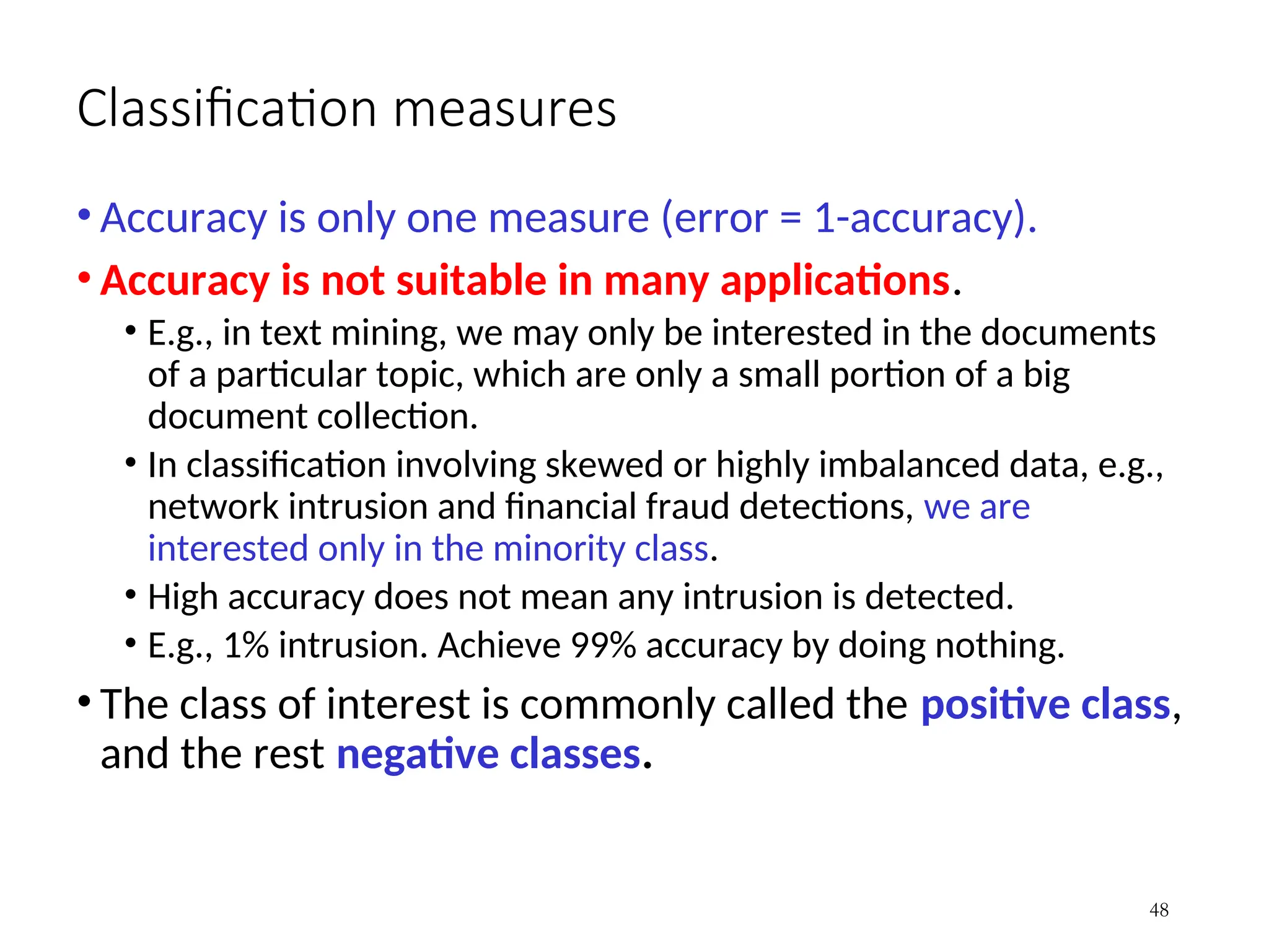
Classification measures
• Accuracyis only one measure (error = 1-accuracy).
• Accuracy is not suitable in many applications.
• E.g., in text mining, we may only be interested in the documents
of a particular topic, which are only a small portion of a big
document collection.
• In classification involving skewed or highly imbalanced data, e.g.,
network intrusion and financial fraud detections, we are
interested only in the minority class.
• High accuracy does not mean any intrusion is detected.
• E.g., 1% intrusion. Achieve 99% accuracy by doing nothing.
• The class of interest is commonly called the positive class,
and the rest negative classes.
48
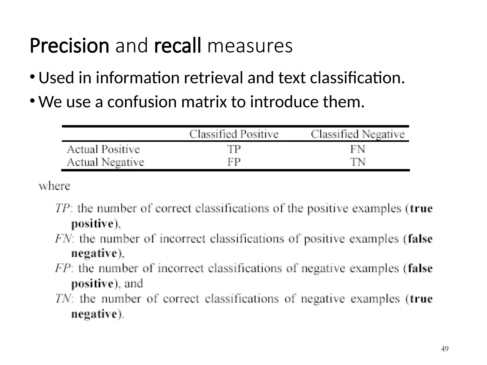
49.
Precision and recallmeasures
• Used in information retrieval and text classification.
• We use a confusion matrix to introduce them.
49
50.
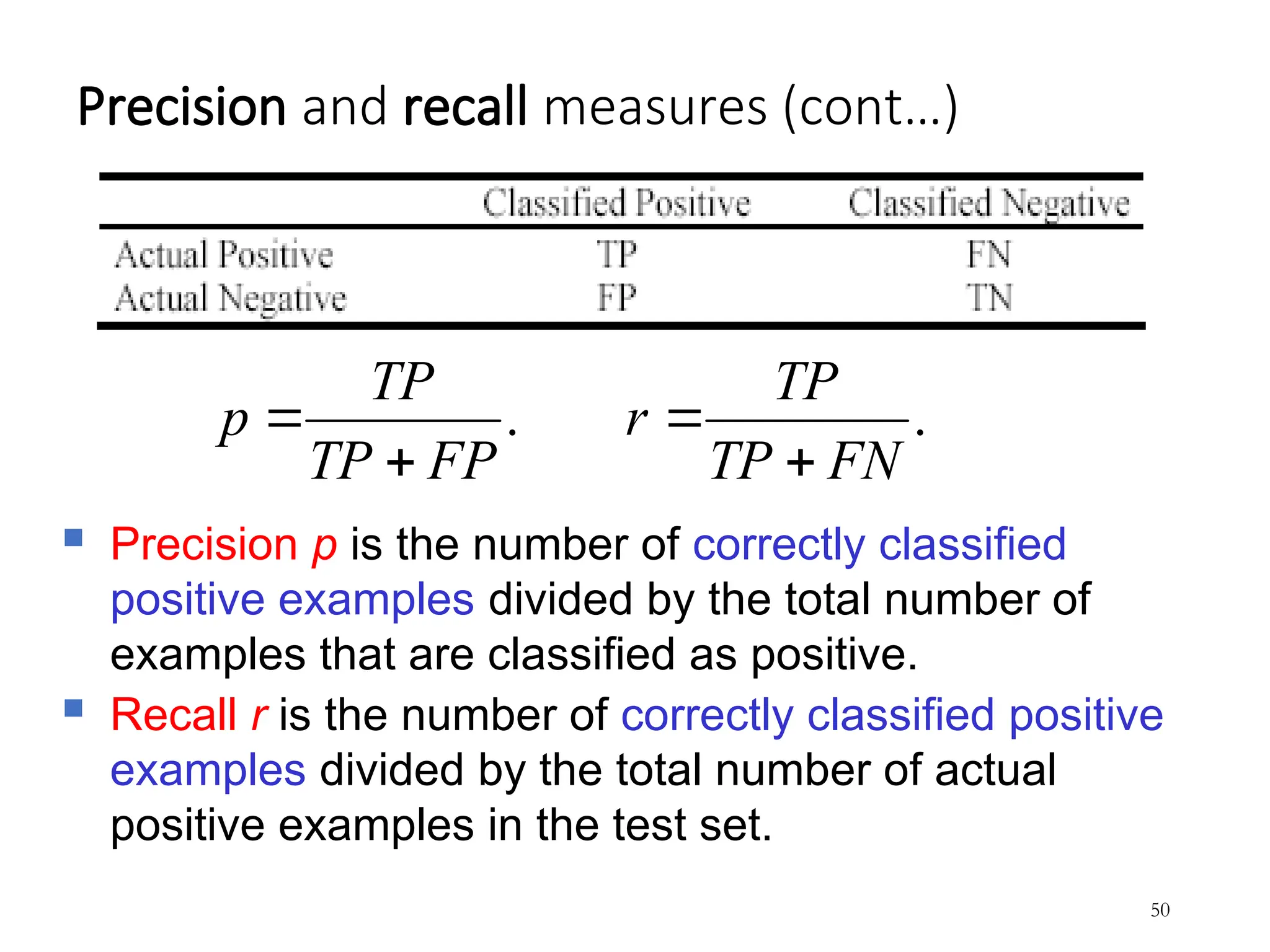
Precision and recallmeasures (cont…)
50
Precision p is the number of correctly classified
positive examples divided by the total number of
examples that are classified as positive.
Recall r is the number of correctly classified positive
examples divided by the total number of actual
positive examples in the test set.
.
.
FN
TP
TP
r
FP
TP
TP
p
51.
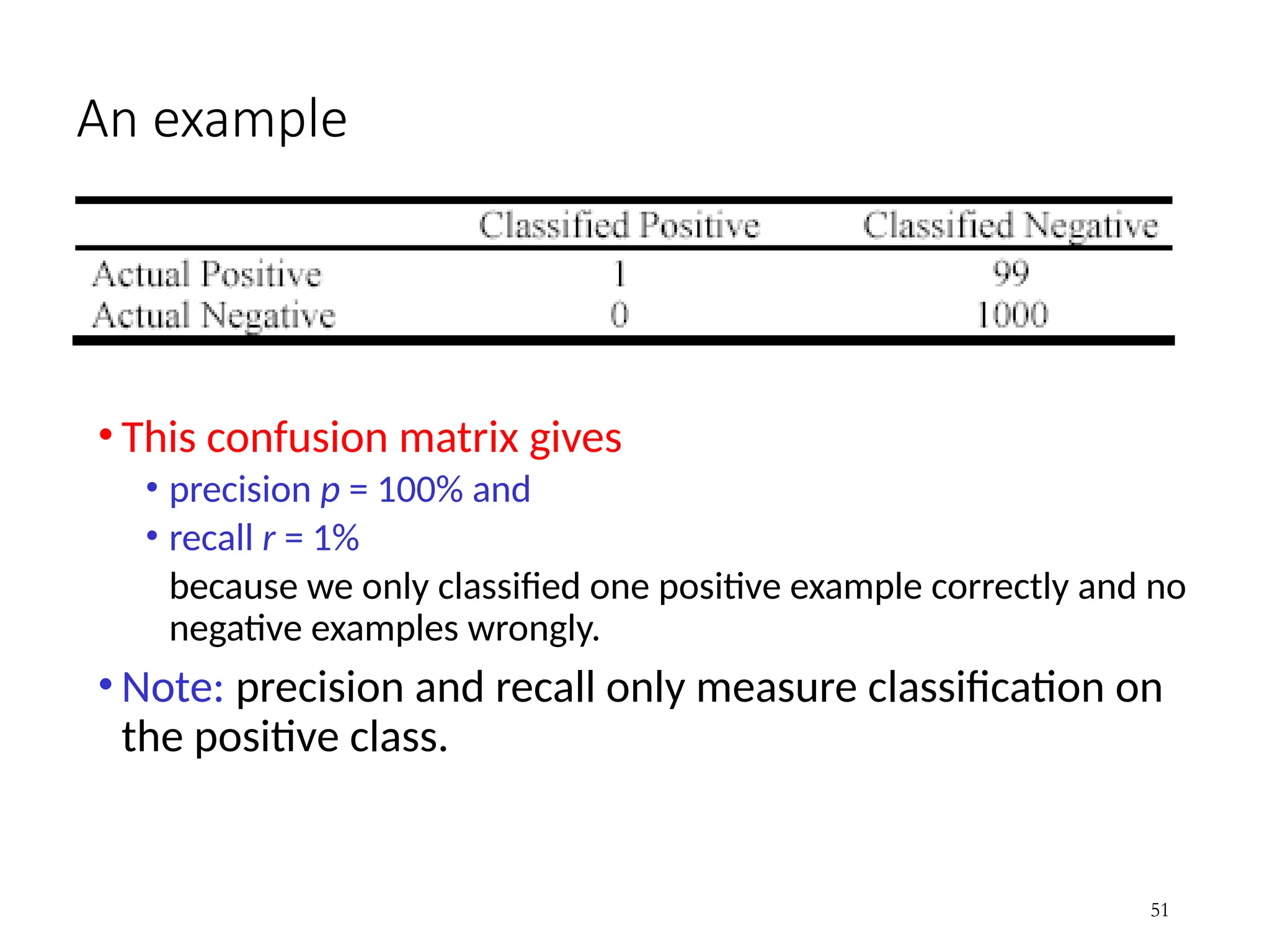
An example
• Thisconfusion matrix gives
• precision p = 100% and
• recall r = 1%
because we only classified one positive example correctly and no
negative examples wrongly.
• Note: precision and recall only measure classification on
the positive class.
51
52.
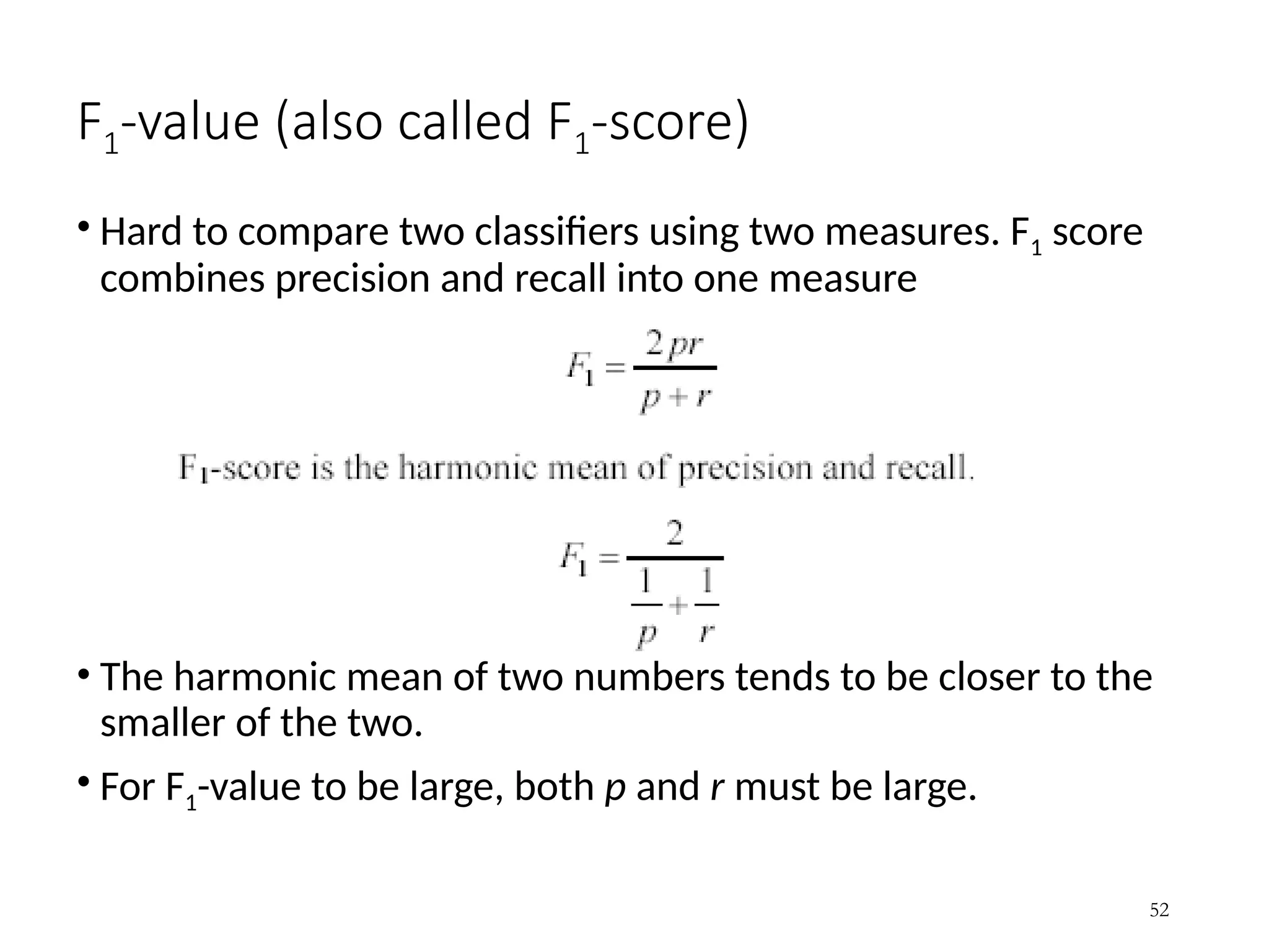
F1-value (also calledF1-score)
• Hard to compare two classifiers using two measures. F1 score
combines precision and recall into one measure
• The harmonic mean of two numbers tends to be closer to the
smaller of the two.
• For F1-value to be large, both p and r must be large.
52
53.
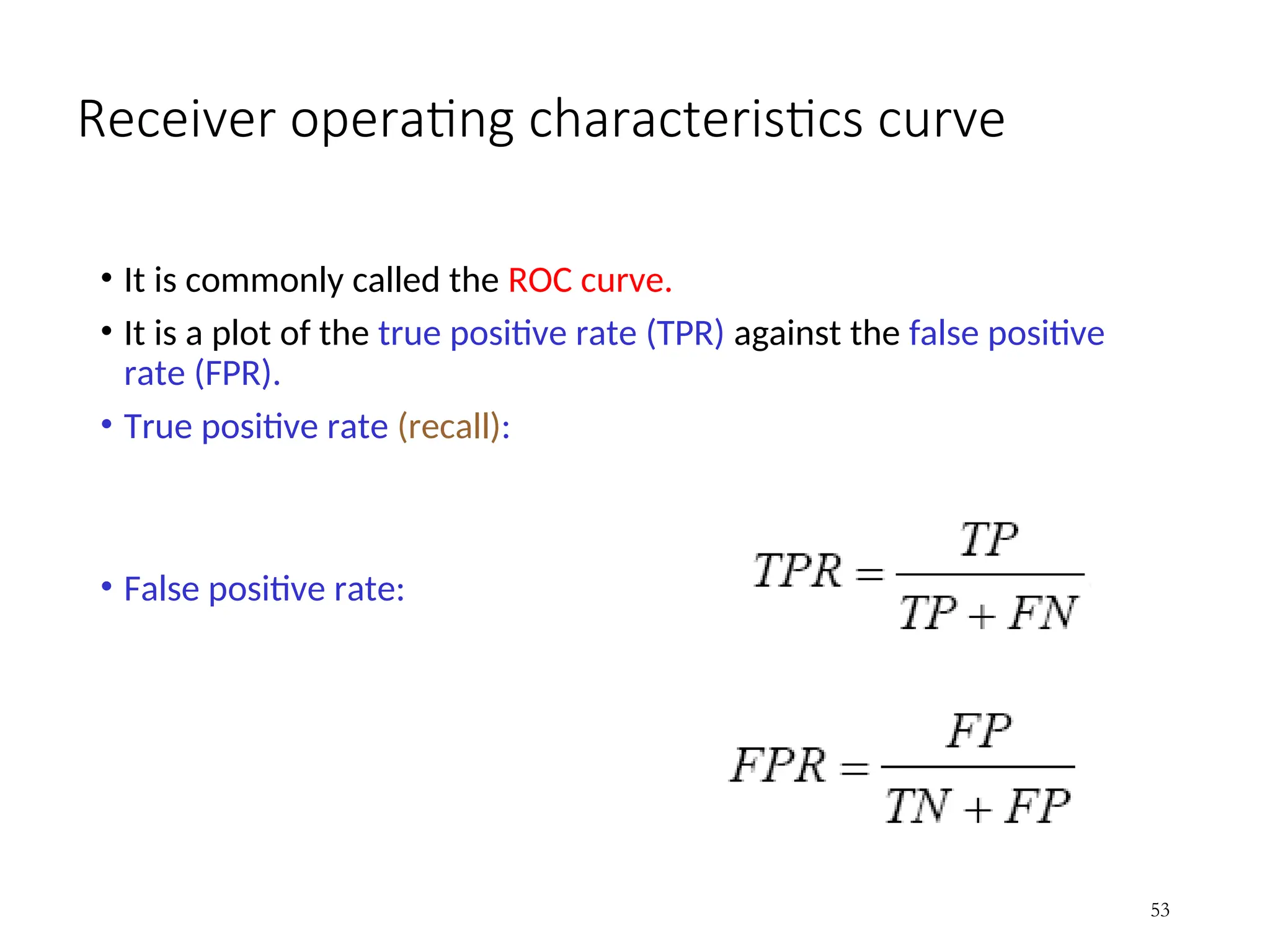
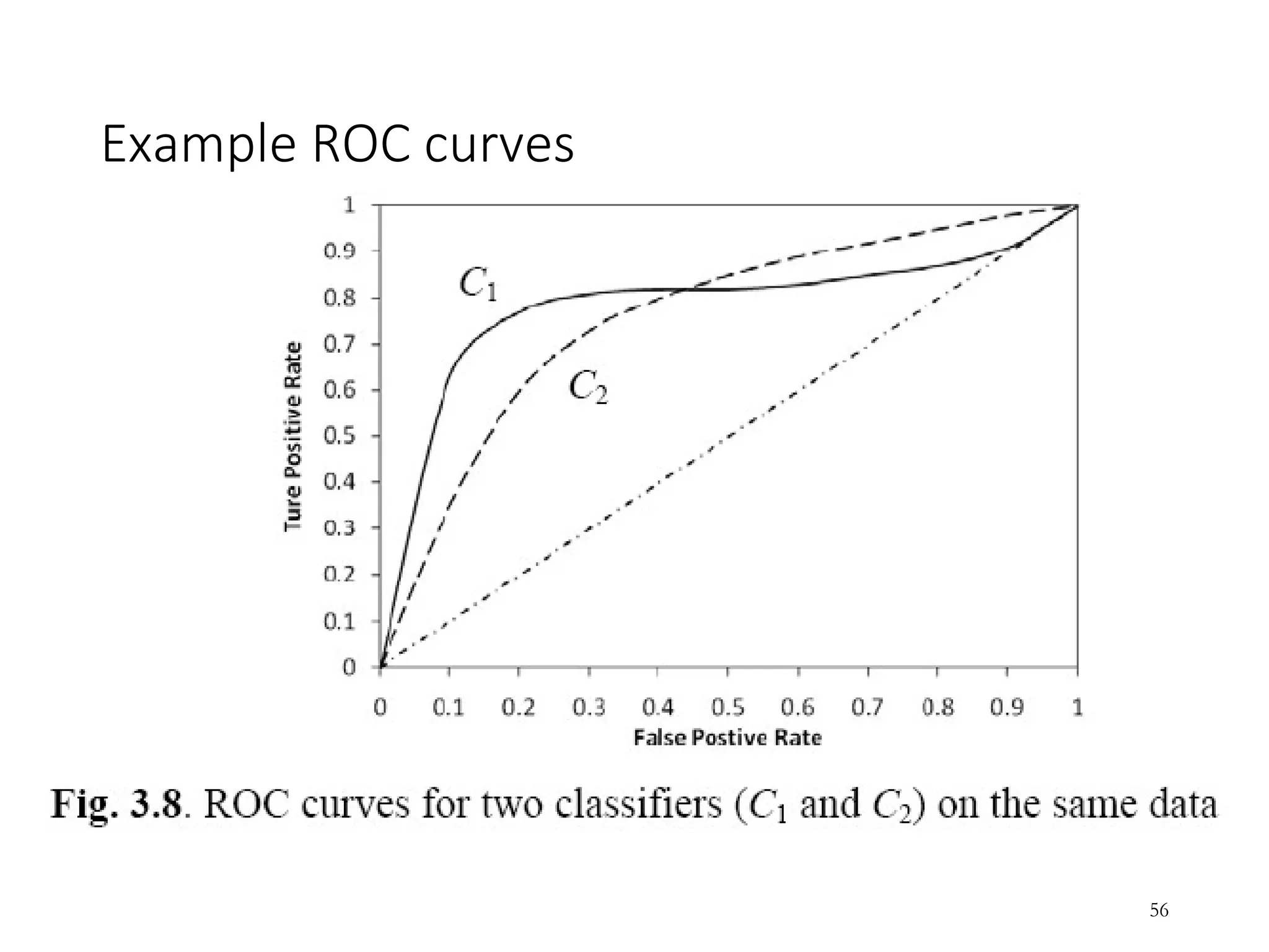
Receiver operating characteristicscurve
• It is commonly called the ROC curve.
• It is a plot of the true positive rate (TPR) against the false positive
rate (FPR).
• True positive rate (recall):
• False positive rate:
53
54.
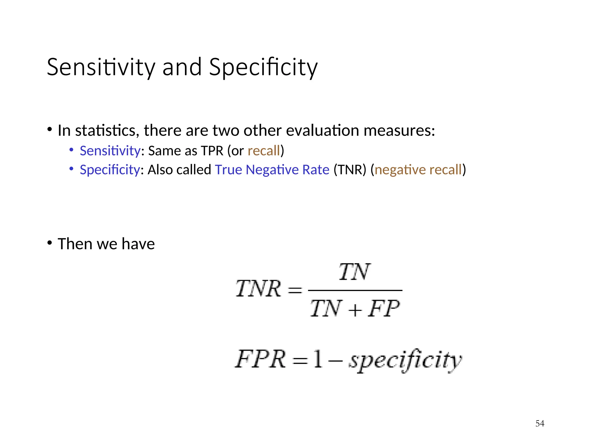
Sensitivity and Specificity
•In statistics, there are two other evaluation measures:
• Sensitivity: Same as TPR (or recall)
• Specificity: Also called True Negative Rate (TNR) (negative recall)
• Then we have
54
55.
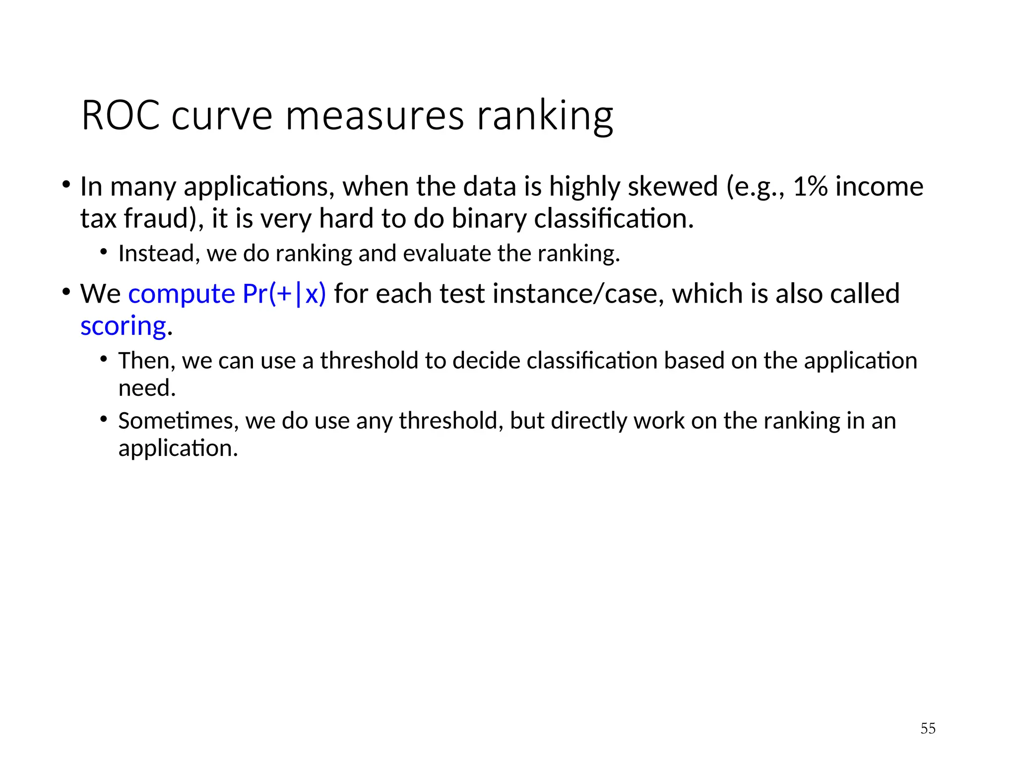
ROC curve measuresranking
• In many applications, when the data is highly skewed (e.g., 1% income
tax fraud), it is very hard to do binary classification.
• Instead, we do ranking and evaluate the ranking.
• We compute Pr(+|x) for each test instance/case, which is also called
scoring.
• Then, we can use a threshold to decide classification based on the application
need.
• Sometimes, we do use any threshold, but directly work on the ranking in an
application.
55
Area Under theCurve (AUC)
• Which classifier is better, C1 or C2?
• It depends on which region you talk about.
• Can we have one measure?
• Yes, we compute the area under the curve (AUC)
• If AUC for Ci is greater than that of Cj, it is said that Ci is better than Cj.
• If a classifier is perfect, its AUC value is 1
• If a classifier makes all random guesses, its AUC value is 0.5.
57
Road Map
• Basicconcepts
• Decision tree induction
• Evaluation of classifiers
• Naïve Bayesian classification
• Naïve Bayes for text classification
• Support vector machines
• Linear regression and gradient descent
• Neural networks
• Summary K-nearest neighbor
• Ensemble methods
• Summary
59
60.
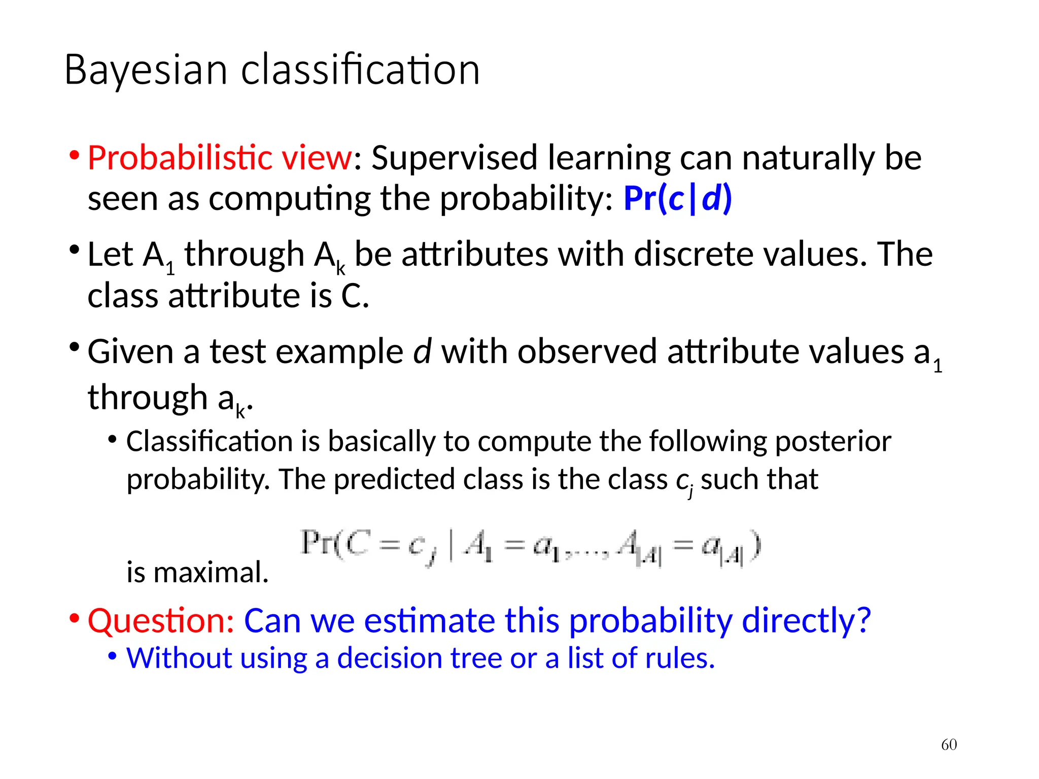
Bayesian classification
• Probabilisticview: Supervised learning can naturally be
seen as computing the probability: Pr(c|d)
• Let A1 through Ak be attributes with discrete values. The
class attribute is C.
• Given a test example d with observed attribute values a1
through ak.
• Classification is basically to compute the following posterior
probability. The predicted class is the class cj such that
is maximal.
• Question: Can we estimate this probability directly?
• Without using a decision tree or a list of rules.
60
61.
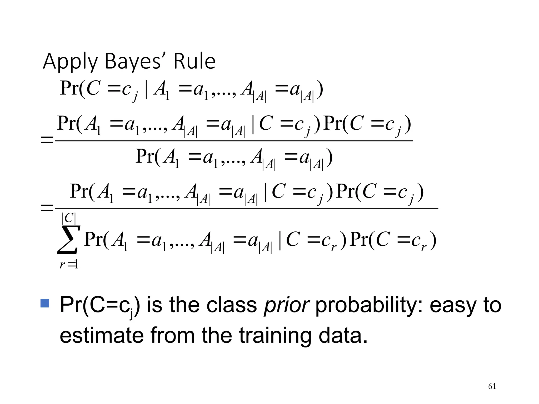
Apply Bayes’ Rule
61
Pr(C=cj) is the class prior probability: easy to
estimate from the training data.
|
|
1
|
|
|
|
1
1
|
|
|
|
1
1
|
|
|
|
1
1
|
|
|
|
1
1
|
|
|
|
1
1
)
Pr(
)
|
,...,
Pr(
)
Pr(
)
|
,...,
Pr(
)
,...,
Pr(
)
Pr(
)
|
,...,
Pr(
)
,...,
|
Pr(
C
r
r
r
A
A
j
j
A
A
A
A
j
j
A
A
A
A
j
c
C
c
C
a
A
a
A
c
C
c
C
a
A
a
A
a
A
a
A
c
C
c
C
a
A
a
A
a
A
a
A
c
C
62.
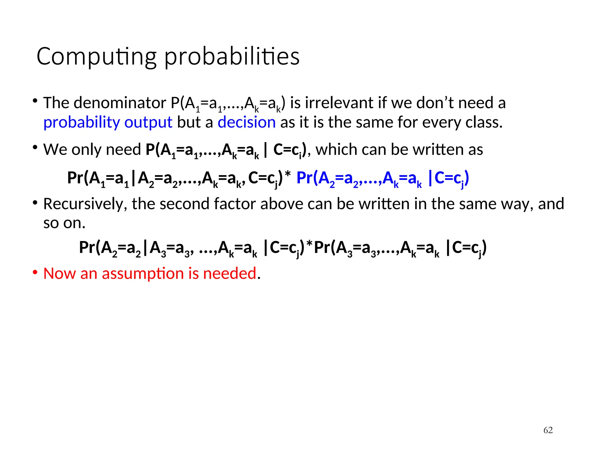
Computing probabilities
• Thedenominator P(A1=a1,...,Ak=ak) is irrelevant if we don’t need a
probability output but a decision as it is the same for every class.
• We only need P(A1=a1,...,Ak=ak | C=ci), which can be written as
Pr(A1=a1|A2=a2,...,Ak=ak,C=cj)* Pr(A2=a2,...,Ak=ak |C=cj)
• Recursively, the second factor above can be written in the same way, and
so on.
Pr(A2=a2|A3=a3, ...,Ak=ak |C=cj)*Pr(A3=a3,...,Ak=ak |C=cj)
• Now an assumption is needed.
62
63.
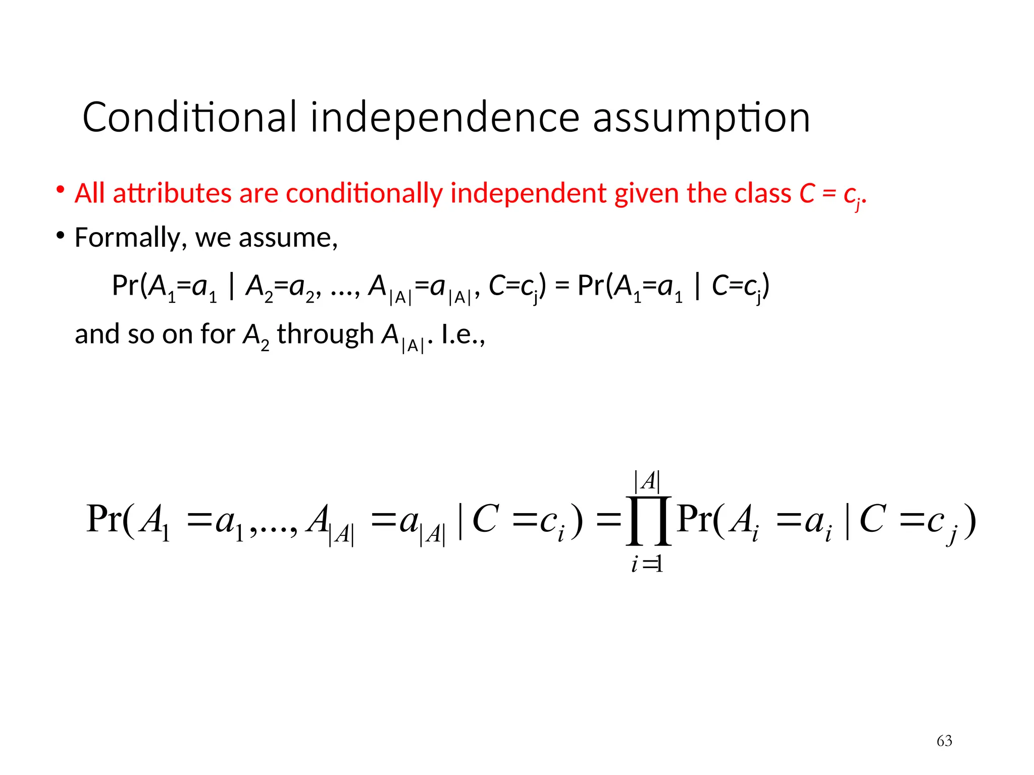
Conditional independence assumption
•All attributes are conditionally independent given the class C = cj.
• Formally, we assume,
Pr(A1=a1 | A2=a2, ..., A|A|=a|A|, C=cj) = Pr(A1=a1 | C=cj)
and so on for A2 through A|A|. I.e.,
63
|
|
1
|
|
|
|
1
1 )
|
Pr(
)
|
,...,
Pr(
A
i
j
i
i
i
A
A c
C
a
A
c
C
a
A
a
A
64.
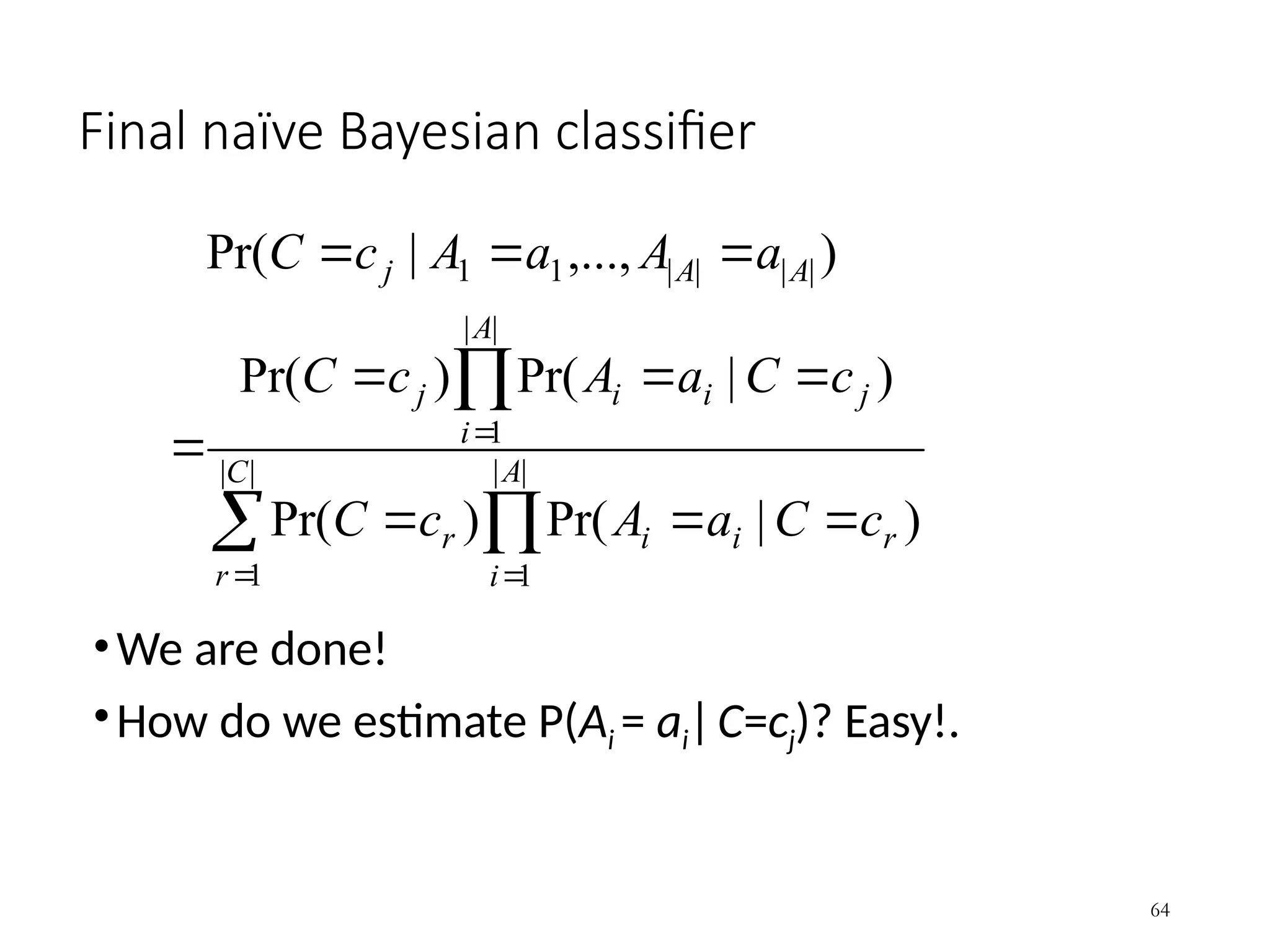
Final naïve Bayesianclassifier
•We are done!
•How do we estimate P(Ai = ai|C=cj)? Easy!.
|
|
1
|
|
1
|
|
1
|
|
|
|
1
1
)
|
Pr(
)
Pr(
)
|
Pr(
)
Pr(
)
,...,
|
Pr(
C
r
A
i
r
i
i
r
A
i
j
i
i
j
A
A
j
c
C
a
A
c
C
c
C
a
A
c
C
a
A
a
A
c
C
64
65.
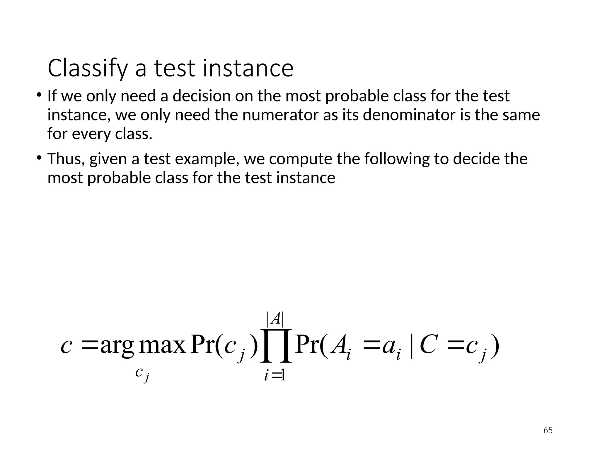
Classify a testinstance
• If we only need a decision on the most probable class for the test
instance, we only need the numerator as its denominator is the same
for every class.
• Thus, given a test example, we compute the following to decide the
most probable class for the test instance
65
|
|
1
)
|
Pr(
)
Pr(
max
arg
A
i
j
i
i
j
c
c
C
a
A
c
c
j
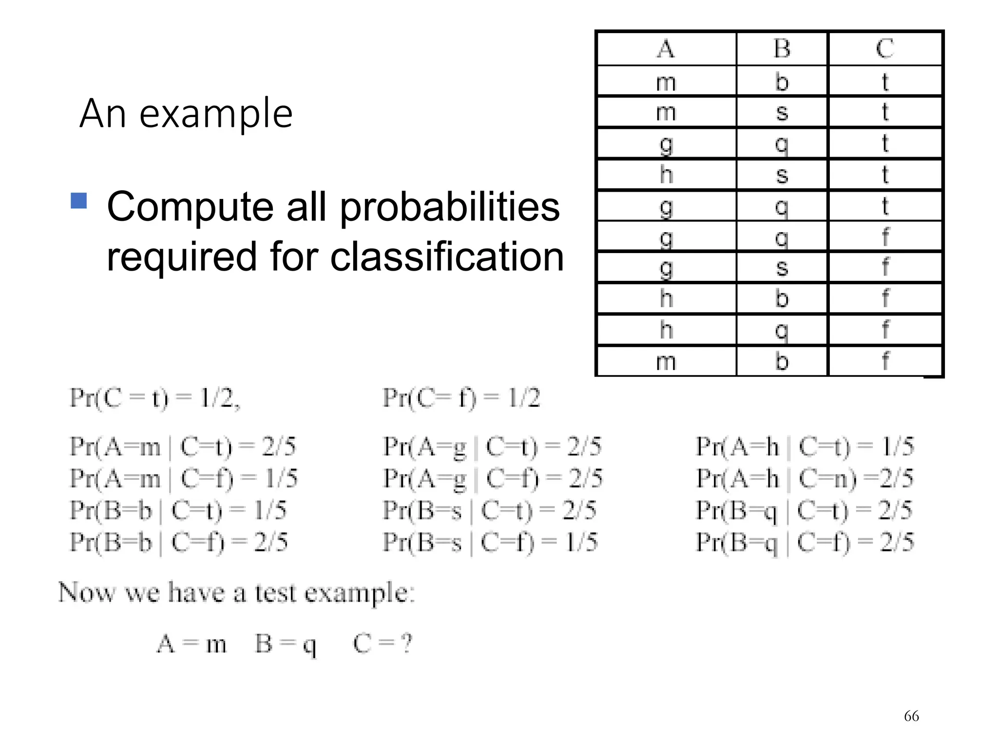
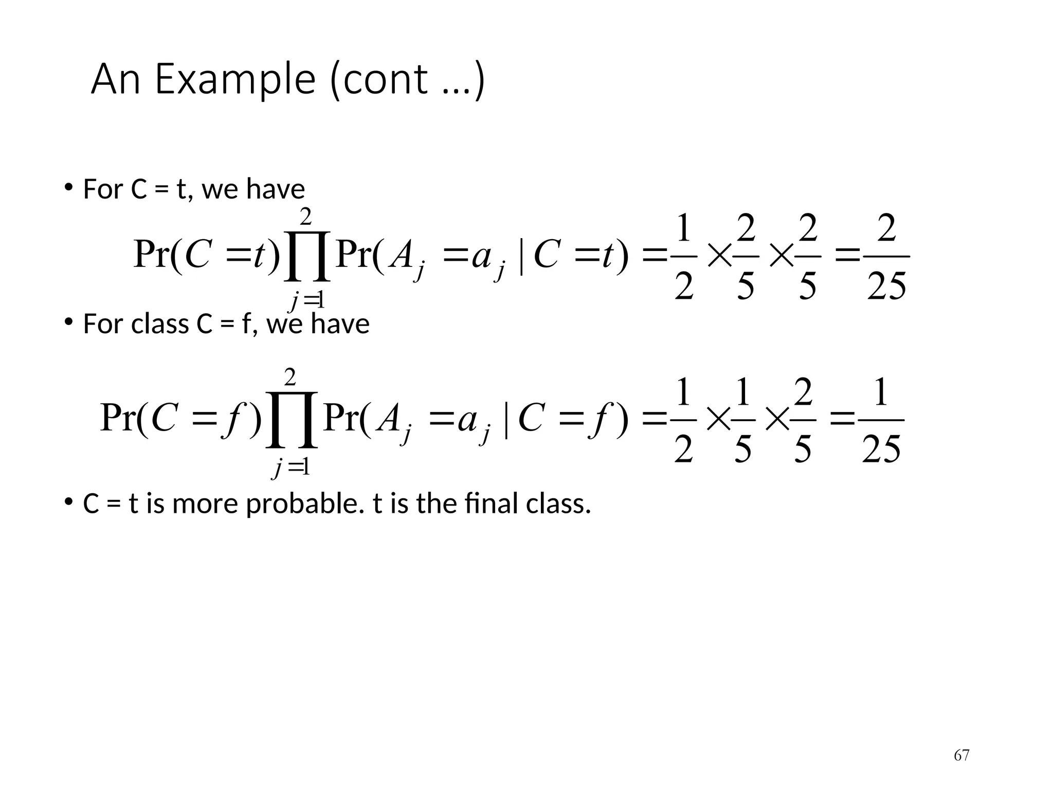
An Example (cont…)
• For C = t, we have
• For class C = f, we have
• C = t is more probable. t is the final class.
67
25
2
5
2
5
2
2
1
)
|
Pr(
)
Pr(
2
1
j
j
j t
C
a
A
t
C
25
1
5
2
5
1
2
1
)
|
Pr(
)
Pr(
2
1
j
j
j f
C
a
A
f
C
68.
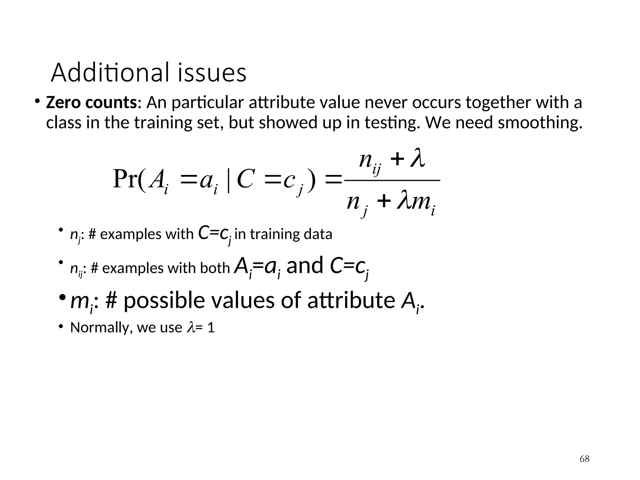
Additional issues
• Zerocounts: An particular attribute value never occurs together with a
class in the training set, but showed up in testing. We need smoothing.
• nj: # examples with C=cj in training data
• nij: # examples with both Ai=ai and C=cj
•mi: # possible values of attribute Ai.
• Normally, we use = 1
68
i
j
ij
j
i
i
m
n
n
c
C
a
A
)
|
Pr(
69.
Additional issues (contd)
•Numeric attributes: Naïve Bayesian learning assumes that all
attributes are categorical. Numeric attributes need to be discretized.
• There are many algorithms, e.g.,
• E.g., use decision tree induction
• Create a data for each numeric attribute A consisting of two columns A and C (class)
• Run the decision tree algorithm to generate intervals for A, which are the resulting
discrete/categorical values.
• Missing values: Ignored
69
70.
On naïve Bayesian(NB) classifier
• Advantages:
• Easy to implement
• Very efficient
• Good results obtained in many applications
• Disadvantages
• Assumption: class conditional independence, therefore loss of accuracy
when the assumption is seriously violated (highly correlated data sets)
• E.g., in a game dataset, decision tree and CBA give 100% accuracy, and NB
only gives 70%.
70
71.
Road Map
• Basicconcepts
• Decision tree induction
• Evaluation of classifiers
• Naïve Bayesian classification
• Naïve Bayes for text classification
• Support vector machines
• Linear regression and gradient descent
• Neural networks
• K-nearest neighbor
• Ensemble methods
• Summary
71
72.
Text classification/categorization
• Dueto the rapid growth of online documents in
organizations and on the Web, automated document
classification has become an important problem.
• Techniques discussed previously can be applied to text
classification, but they are not as effective as the next
three methods.
• We first study a naïve Bayesian method specifically
formulated for texts, which makes use of some text
specific features.
• However, the ideas are similar to the preceding NB
method.
72
73.
Probabilistic framework
• Generativemodel: Each document is generated by a parametric
distribution governed by a set of hidden parameters.
• The generative model makes two assumptions
• The data (or the text documents) are generated by a mixture model,
• There is one-to-one correspondence between mixture components and
document classes.
73
74.
Mixture model
• Amixture model models the data with a number of statistical
distributions.
• Intuitively, each distribution corresponds to a data cluster/class and the
parameters of the distribution provide a description of the corresponding
cluster.
• Each distribution in a mixture model is also called a mixture component.
• The distribution/component can be of any kind.
74
75.
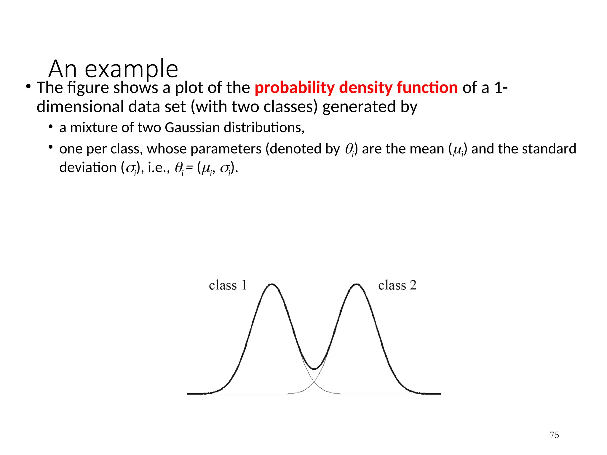
An example
• Thefigure shows a plot of the probability density function of a 1-
dimensional data set (with two classes) generated by
• a mixture of two Gaussian distributions,
• one per class, whose parameters (denoted by i) are the mean (i) and the standard
deviation (i), i.e., i = (i, i).
75
76.
Mixture model (cont…)
• Let the number of mixture components (or distributions) in a mixture
model be K.
• Let the jth distribution have the parameters j.
• Let be the set of parameters of all components, = {1, 2, …, K, 1,
2, …, K}, where j is the mixture weight (or mixture probability) of the
mixture component j and j is the parameters of component j.
• How does the model generate documents?
76
77.
Document generation
• Dueto one-to-one correspondence, each class
corresponds to a mixture component. The mixture
weights are class prior probabilities, i.e., j = Pr(cj|).
• The mixture model generates each document di by:
• first selecting a mixture component (or class) according to class
prior probabilities (i.e., mixture weights), j = Pr(cj|).
• then having this selected mixture component (cj) generate a
document di according to its parameters, with distribution Pr(di|cj;
) or more precisely Pr(di|cj; j).
77
)
;
|
Pr(
)
Θ
|
Pr(
)
|
Pr(
|
|
1
C
j
j
i
j
i c
d
c
d (23)
78.
Model text documents
•The naïve Bayesian classification treats each document as a “bag of
words”. The generative model makes the following further assumptions:
• Words of a document are generated independently of context given the class
label. The familiar naïve Bayes assumption used before.
• The probability of a word is independent of its position in the document. The
document length is chosen independent of its class.
78
79.
Multinomial distribution
•With theassumptions, each document can be
regarded as generated by a multinomial distr.
•Multinomial trial: a process resulting k (>=2) outcomes
with probability p1, …, pk.
• Rolling of a dice is a multinomial trial. A fair dice with 6 faces
(outcomes) has p1 = p2= …= p6 =1/6.
•Let Xi be the # of trials resulted in ith outcome
•The collection of discrete random variables X1, …, Xk is
said to have the multinomial distribution with
parameters n, p1, …, pk. (n: total # of trials)
79
80.
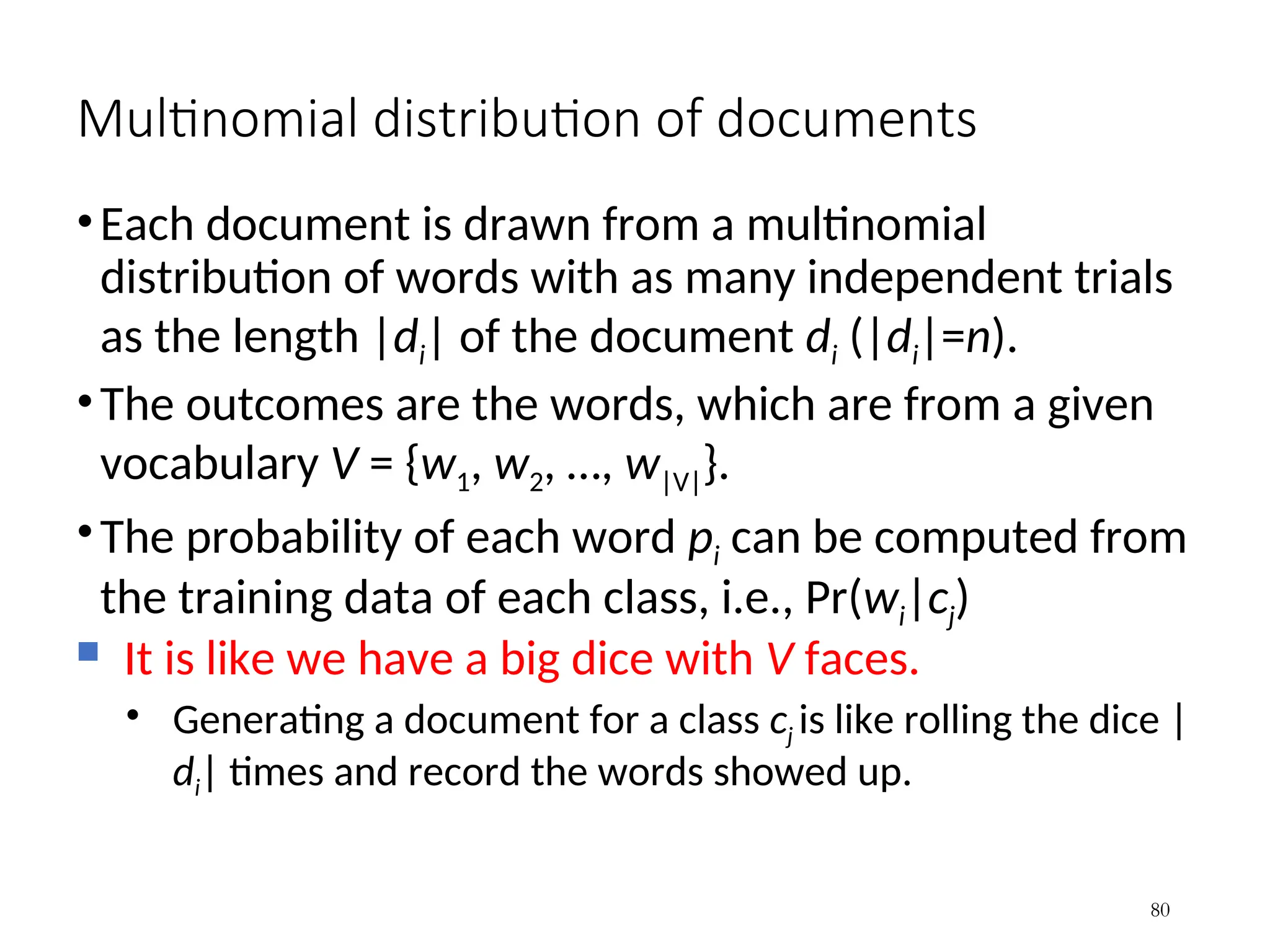
Multinomial distribution ofdocuments
•Each document is drawn from a multinomial
distribution of words with as many independent trials
as the length |di| of the document di (|di|=n).
•The outcomes are the words, which are from a given
vocabulary V = {w1, w2, …, w|V|}.
•The probability of each word pi can be computed from
the training data of each class, i.e., Pr(wi|cj)
It is like we have a big dice with V faces.
• Generating a document for a class cj is like rolling the dice |
di| times and record the words showed up.
80
81.
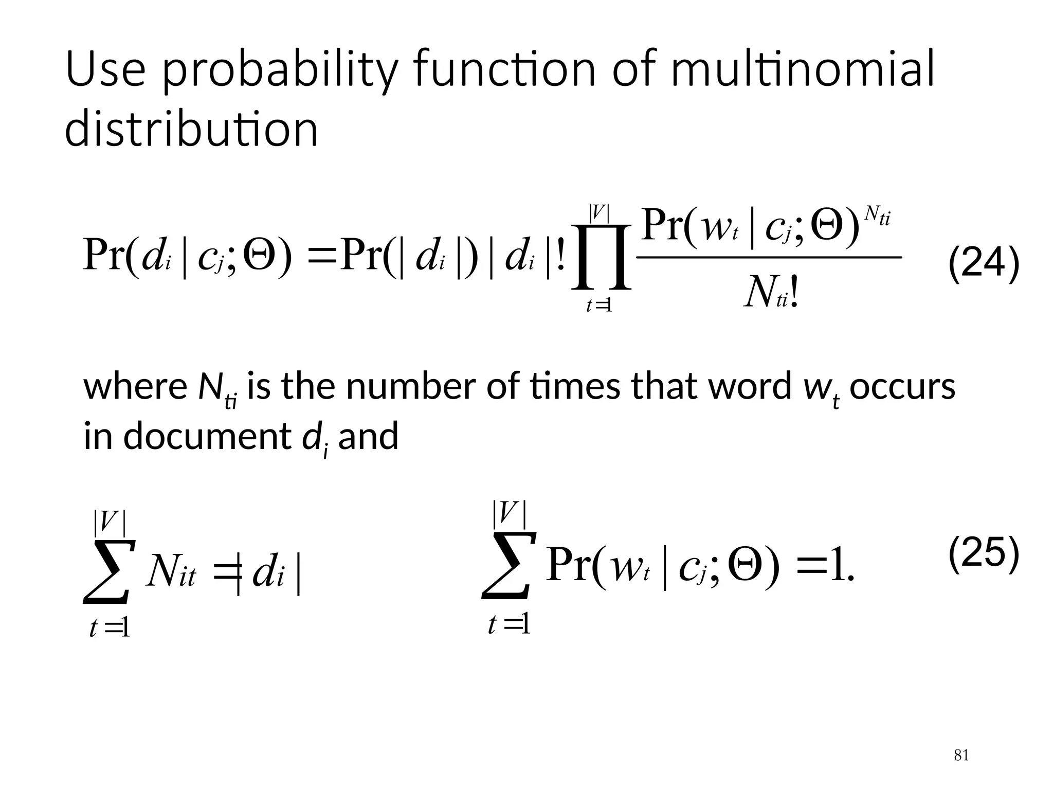
Use probability functionof multinomial
distribution
where Nti is the number of times that word wt occurs
in document di and
81
|
|
1 !
)
;
|
Pr(
|!
|
|)
Pr(|
)
;
|
Pr(
V
t ti
ti
N
j
t
i
i
j
i
N
c
w
d
d
c
d
|
|
|
|
1
i
V
t
it d
N
.
1
)
;
|
Pr(
|
|
1
V
t
j
t c
w
(24)
(25)
82.
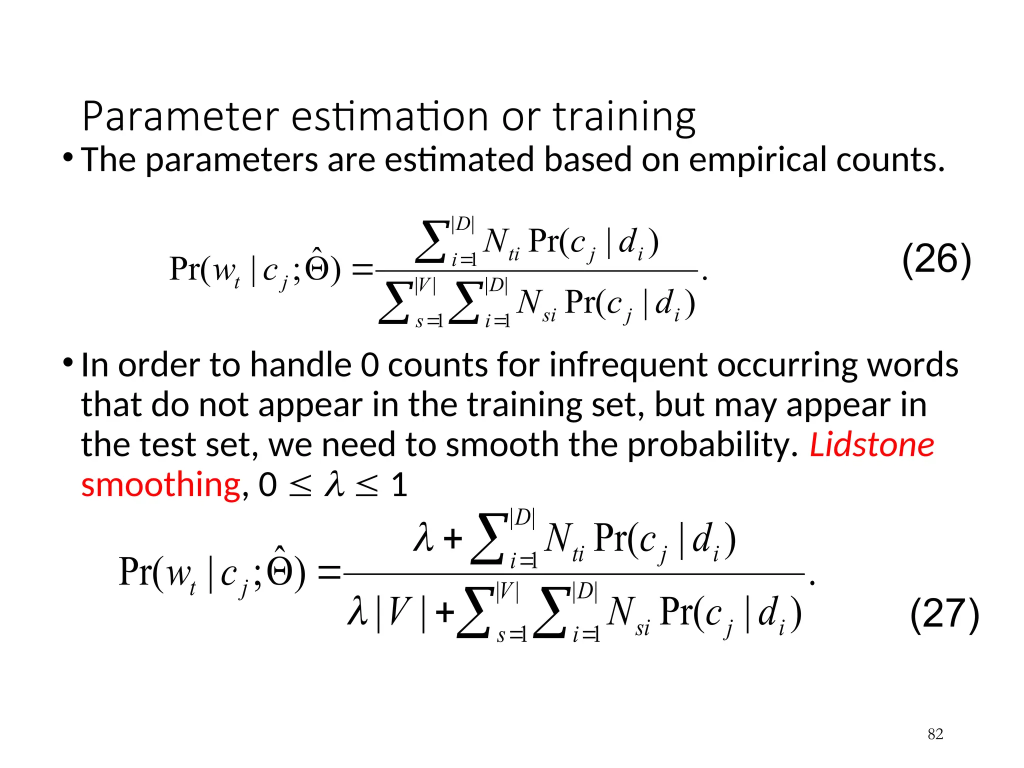
Parameter estimation ortraining
• The parameters are estimated based on empirical counts.
• In order to handle 0 counts for infrequent occurring words
that do not appear in the training set, but may appear in
the test set, we need to smooth the probability. Lidstone
smoothing, 0 1
82
.
)
|
Pr(
)
|
Pr(
)
ˆ
;
|
Pr( |
|
1
|
|
1
|
|
1
V
s
D
i i
j
si
D
i i
j
ti
j
t
d
c
N
d
c
N
c
w
.
)
|
Pr(
|
|
)
|
Pr(
)
ˆ
;
|
Pr( |
|
1
|
|
1
|
|
1
V
s
D
i i
j
si
D
i i
j
ti
j
t
d
c
N
V
d
c
N
c
w
(26)
(27)
83.
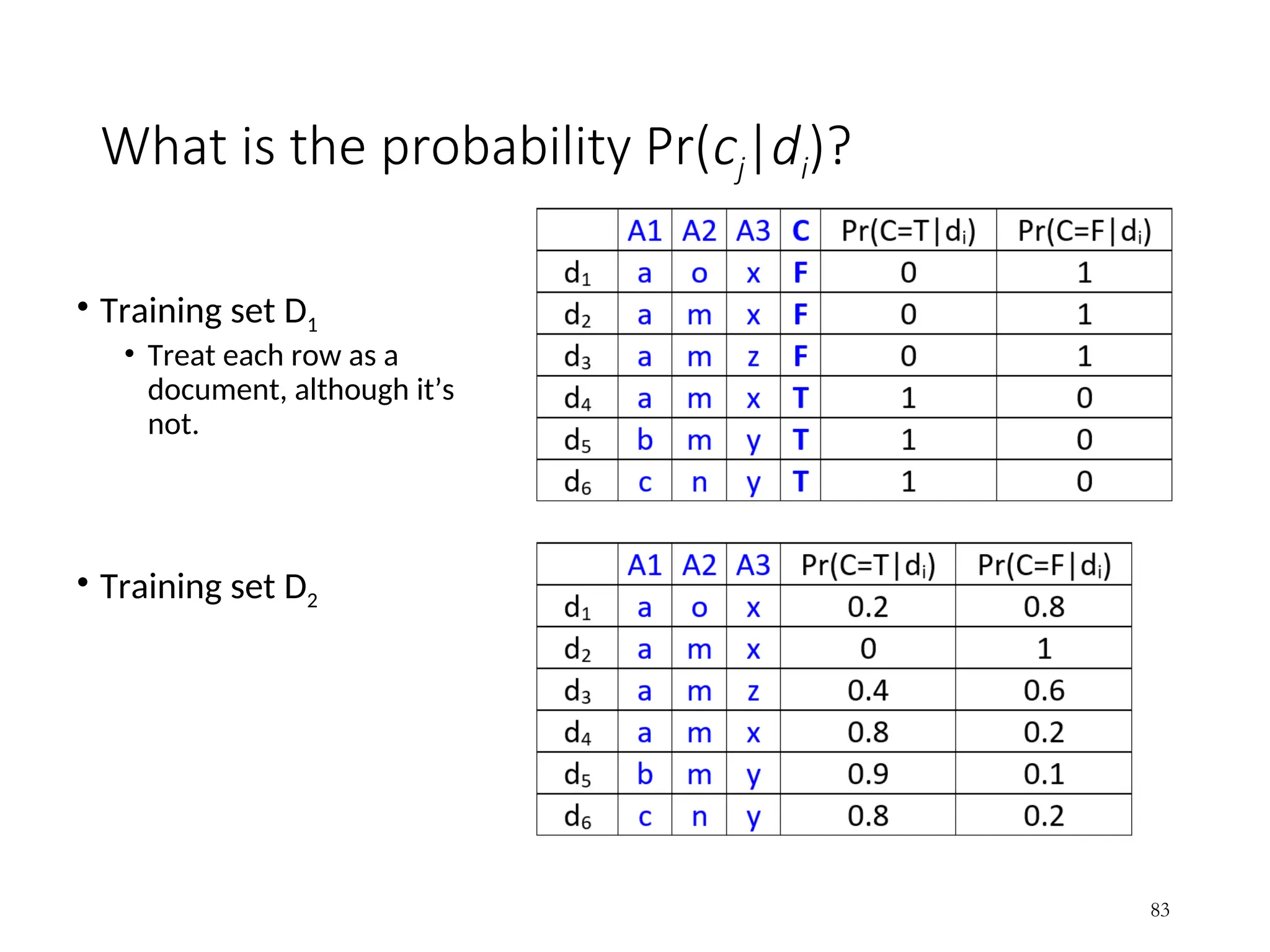
What is theprobability Pr(cj|di)?
• Training set D1
• Treat each row as a
document, although it’s
not.
• Training set D2
83
84.
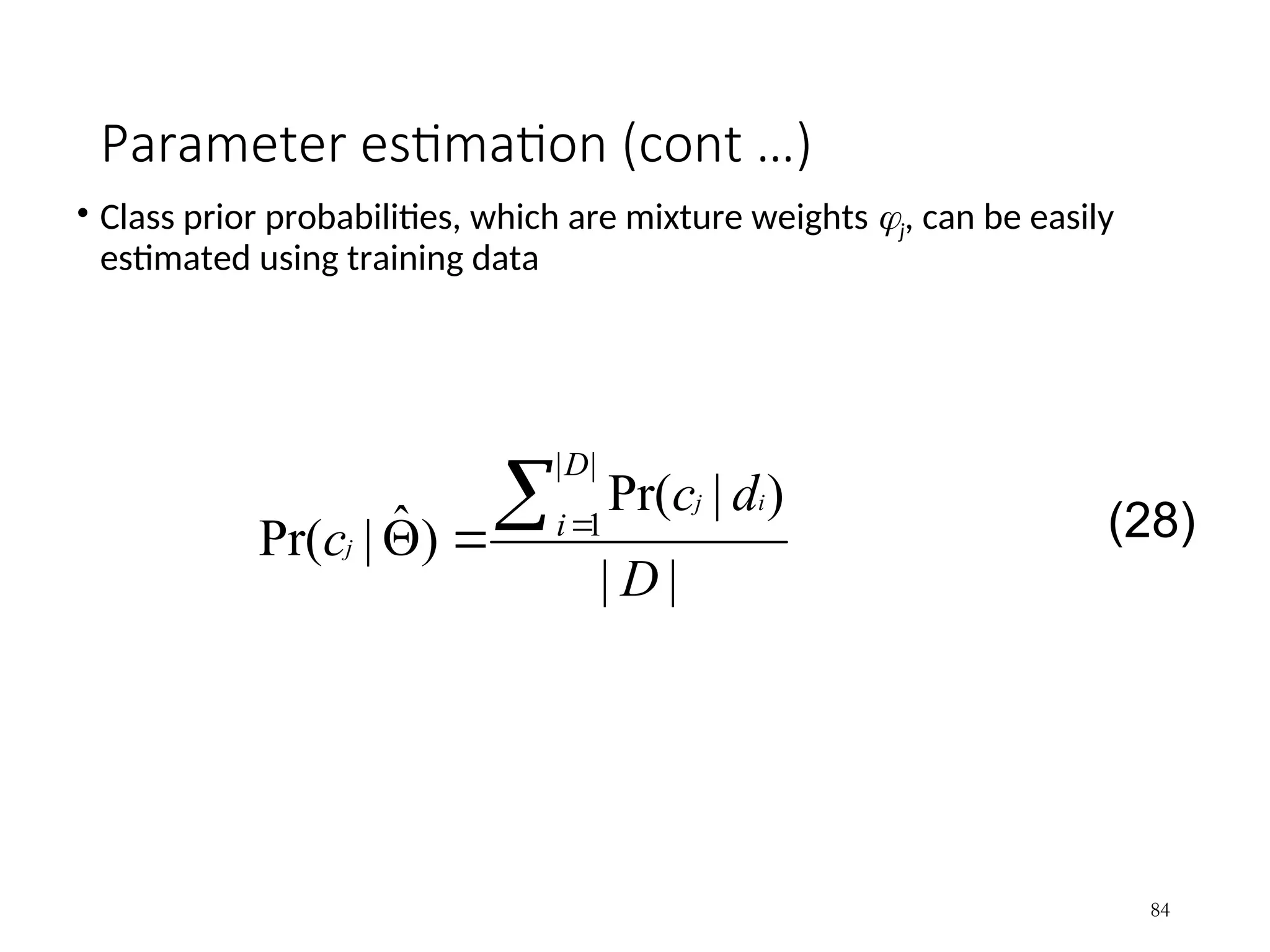
Parameter estimation (cont…)
• Class prior probabilities, which are mixture weights j, can be easily
estimated using training data
84
|
|
)
|
Pr(
)
ˆ
|
Pr(
|
|
1
D
d
c
c
D
i
i
j
j
(28)
85.
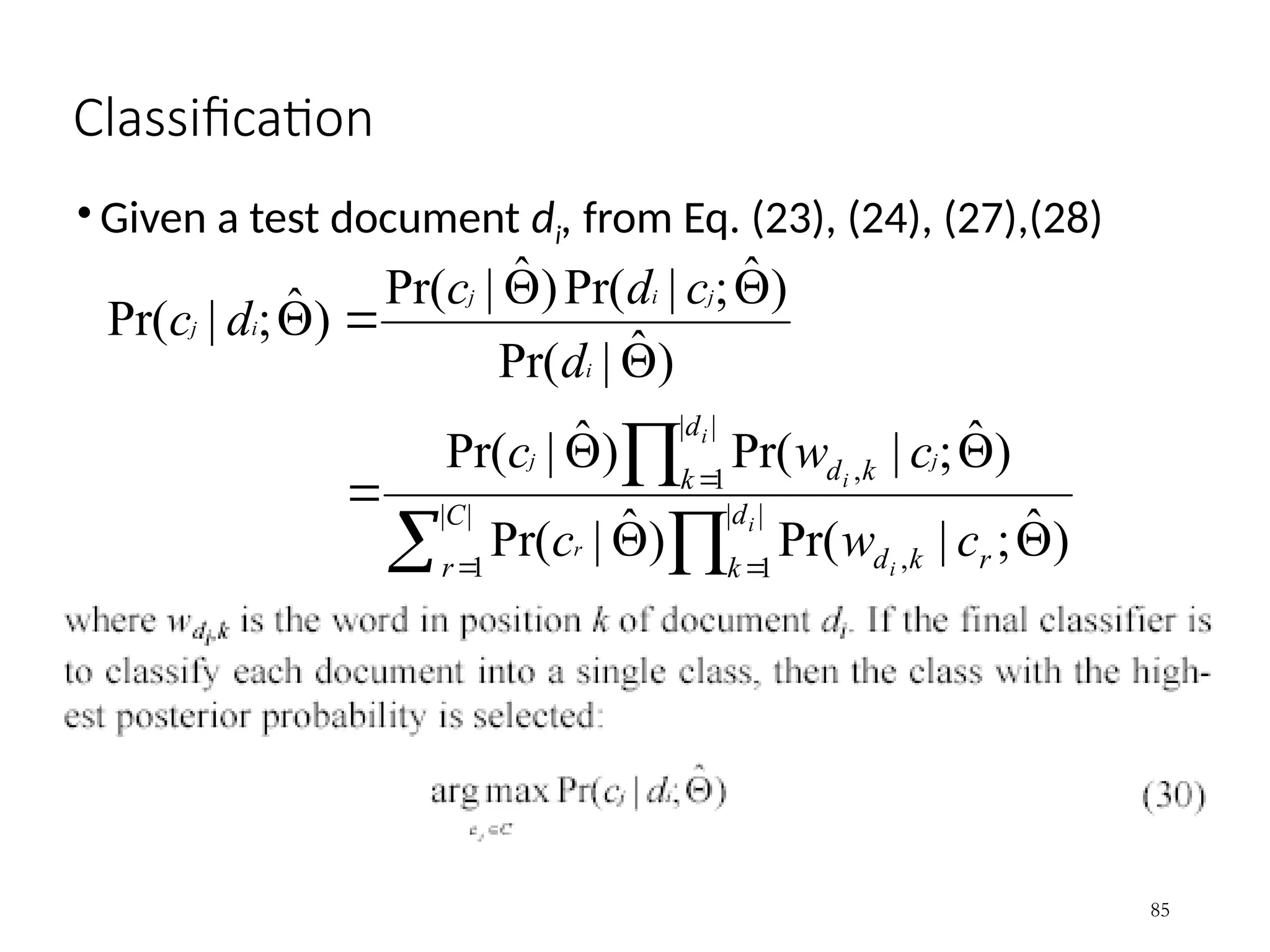
Classification
• Given atest document di, from Eq. (23), (24), (27),(28)
85
|
|
1
|
|
1 ,
|
|
1 ,
)
ˆ
;
|
Pr(
)
ˆ
|
Pr(
)
ˆ
;
|
Pr(
)
ˆ
|
Pr(
)
ˆ
|
Pr(
)
ˆ
;
|
Pr(
)
ˆ
|
Pr(
)
ˆ
;
|
Pr(
C
r
d
k r
k
d
d
k k
d
i
i
r
i
j
i
j
i
j
i
j
i
j
c
w
c
c
w
c
d
c
d
c
d
c
86.
Discussions
• Most assumptionsmade by naïve Bayesian learning are violated to some
degree in practice.
• Despite such violations, researchers have shown that naïve Bayesian
learning produces very accurate models.
• The main problem is the mixture model assumption.
• When this assumption is seriously violated, the classification performance can be
poor.
• Naïve Bayesian learning is extremely efficient.
86
87.
Road Map
• Basicconcepts
• Decision tree induction
• Evaluation of classifiers
• Naïve Bayesian classification
• Naïve Bayes for text classification
• Support vector machines
• Linear regression and gradient descent
• Neural networks
• K-nearest neighbor
• Ensemble methods
• Summary
87
88.
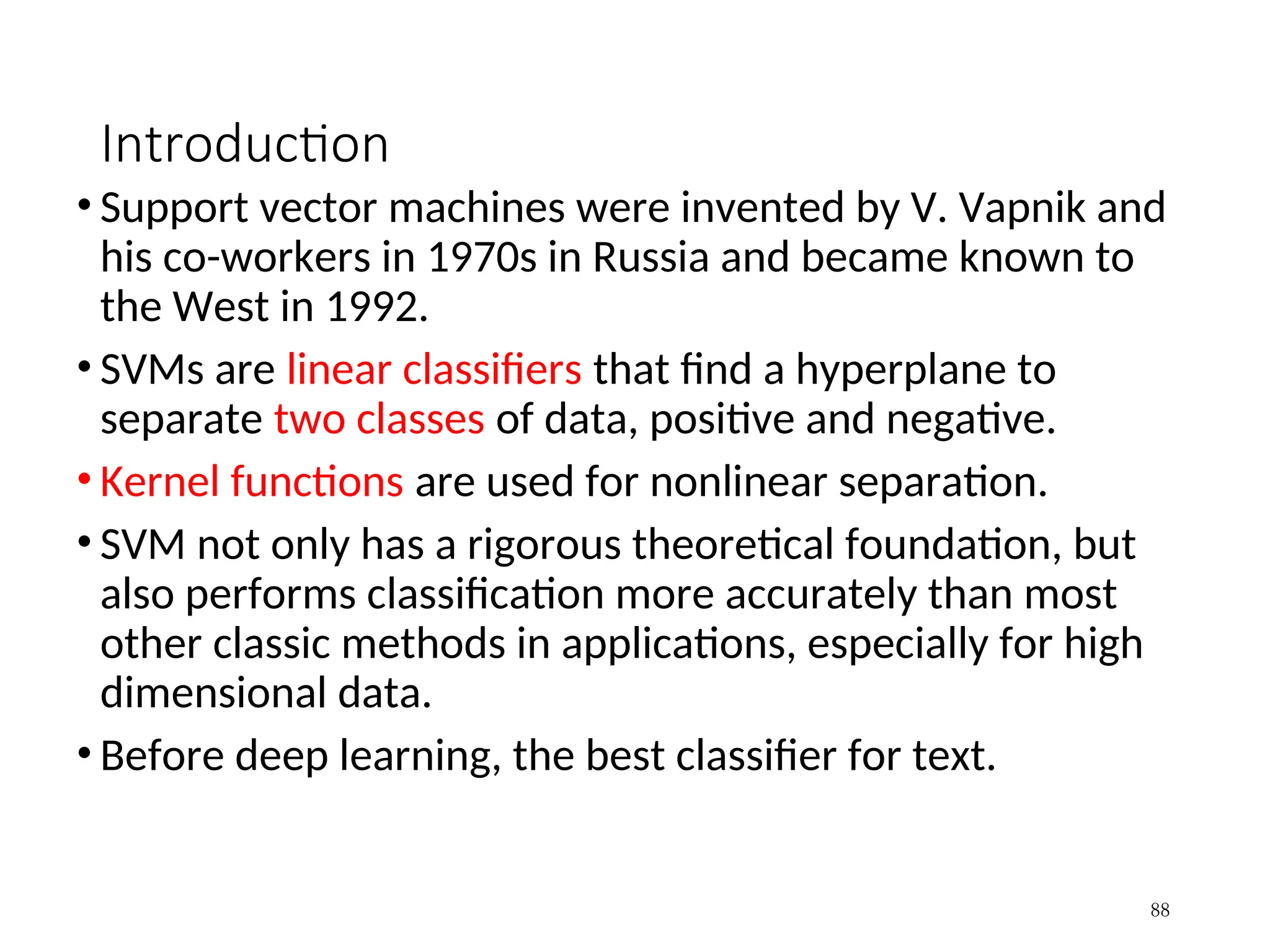
Introduction
• Support vectormachines were invented by V. Vapnik and
his co-workers in 1970s in Russia and became known to
the West in 1992.
• SVMs are linear classifiers that find a hyperplane to
separate two classes of data, positive and negative.
• Kernel functions are used for nonlinear separation.
• SVM not only has a rigorous theoretical foundation, but
also performs classification more accurately than most
other classic methods in applications, especially for high
dimensional data.
• Before deep learning, the best classifier for text.
88
89.
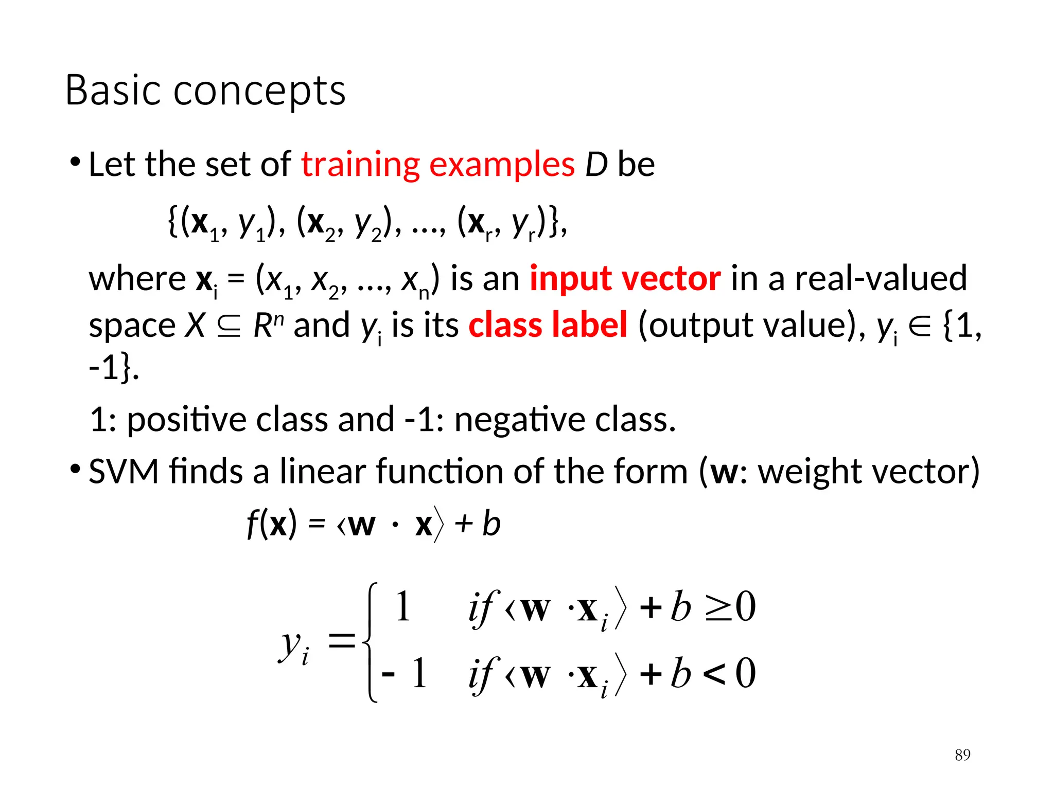
Basic concepts
• Letthe set of training examples D be
{(x1, y1), (x2, y2), …, (xr, yr)},
where xi = (x1, x2, …, xn) is an input vector in a real-valued
space X Rn
and yi is its class label (output value), yi {1,
-1}.
1: positive class and -1: negative class.
• SVM finds a linear function of the form (w: weight vector)
f(x) = w x + b
89
0
1
0
1
b
if
b
if
y
i
i
i
x
w
x
w
90.
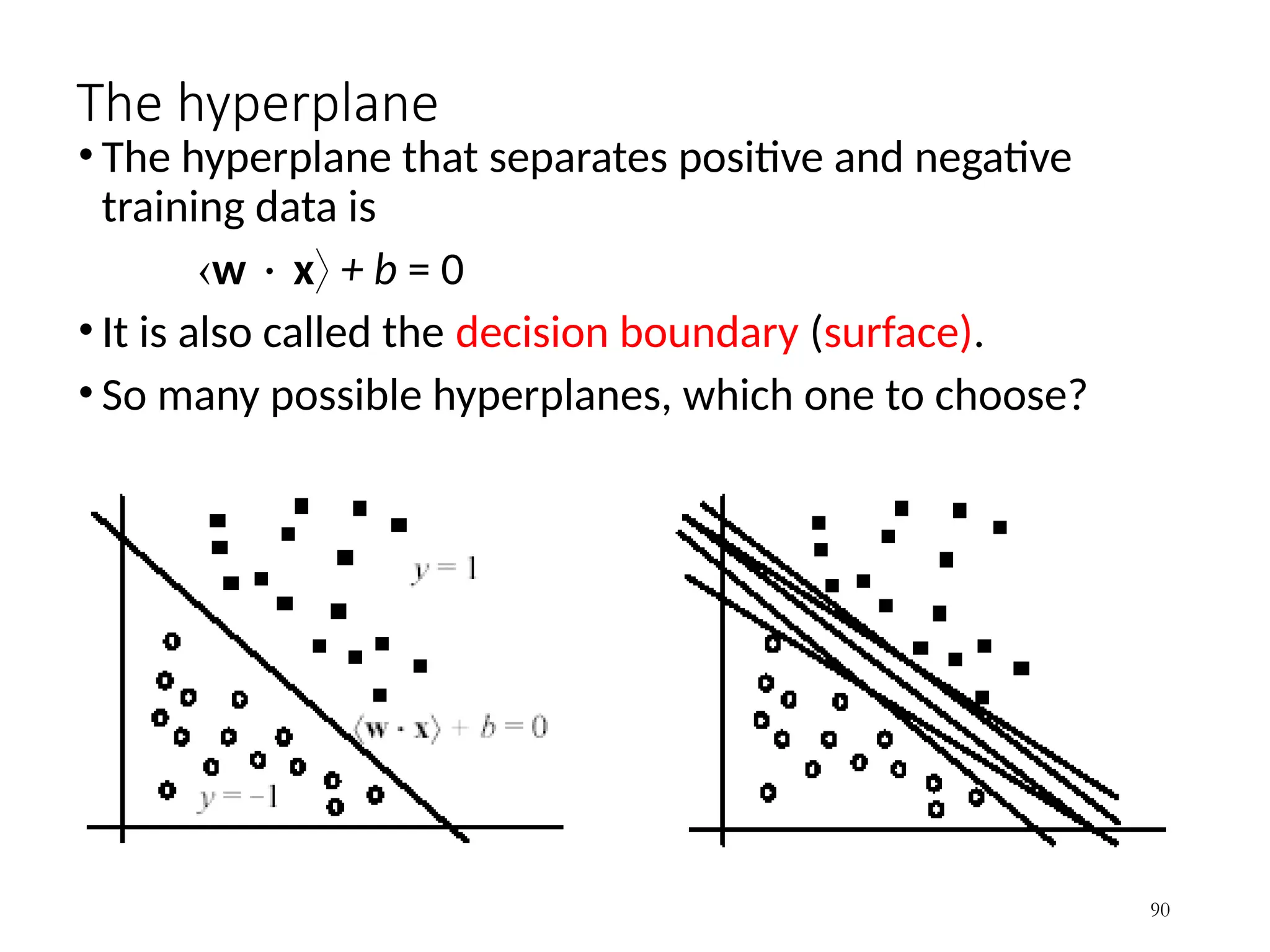
The hyperplane
• Thehyperplane that separates positive and negative
training data is
w x + b = 0
• It is also called the decision boundary (surface).
• So many possible hyperplanes, which one to choose?
90
91.
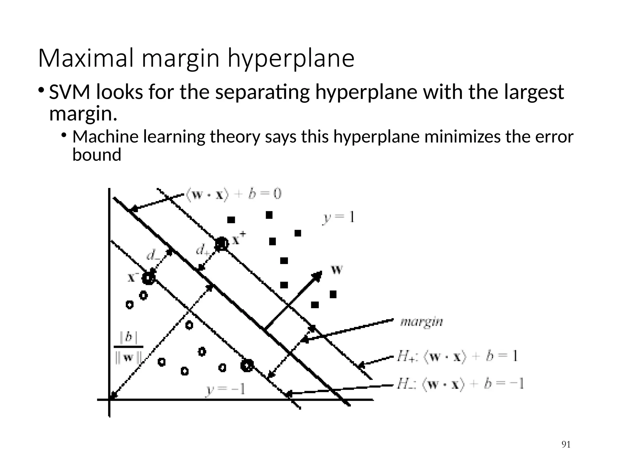
Maximal margin hyperplane
•SVM looks for the separating hyperplane with the largest
margin.
• Machine learning theory says this hyperplane minimizes the error
bound
91
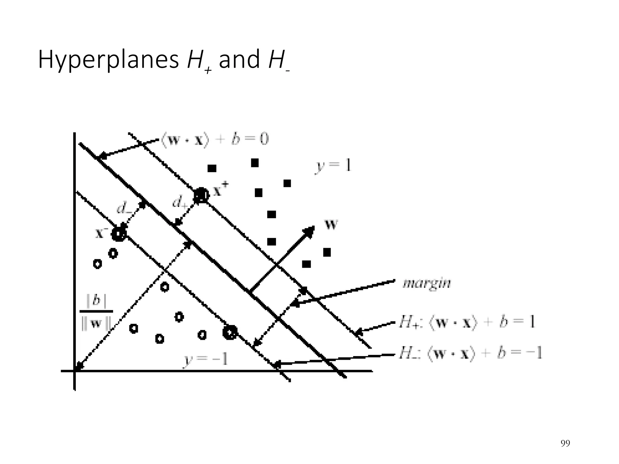
92.
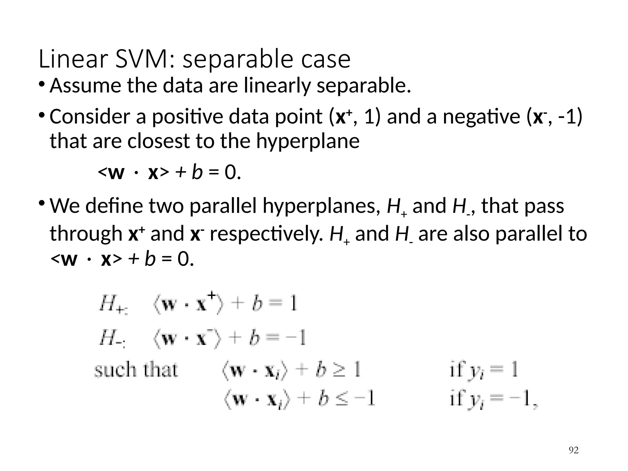
Linear SVM: separablecase
• Assume the data are linearly separable.
• Consider a positive data point (x+
, 1) and a negative (x-
, -1)
that are closest to the hyperplane
<w x> + b = 0.
• We define two parallel hyperplanes, H+ and H-, that pass
through x+
and x-
respectively. H+ and H- are also parallel to
<w x> + b = 0.
92
93.
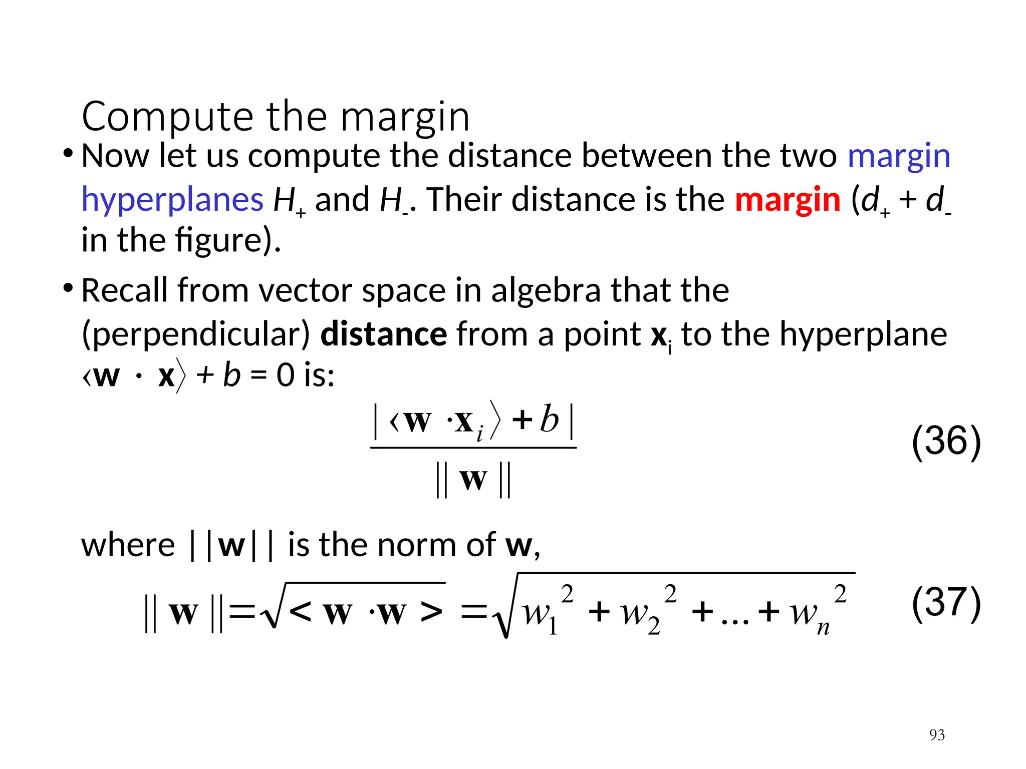
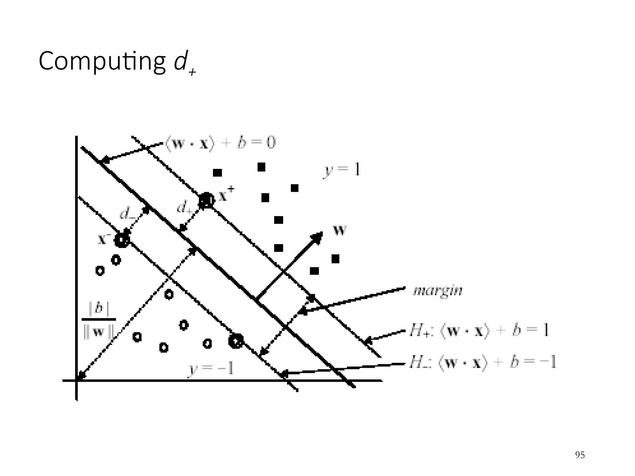
Compute the margin
•Now let us compute the distance between the two margin
hyperplanes H+ and H-. Their distance is the margin (d+ + d
in the figure).
• Recall from vector space in algebra that the
(perpendicular) distance from a point xi to the hyperplane
w x + b = 0 is:
where ||w|| is the norm of w,
93
||
||
|
|
w
x
w b
i
2
2
2
2
1 ...
||
|| n
w
w
w
w
w
w
(36)
(37)
94.
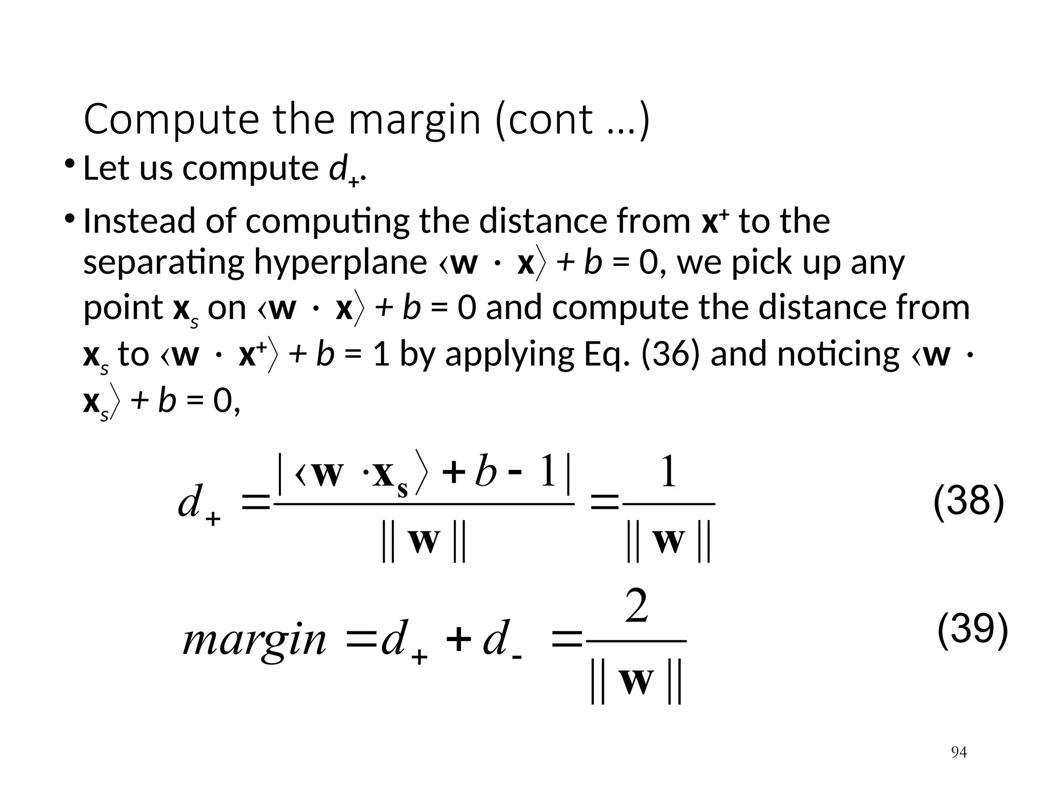
Compute the margin(cont …)
• Let us compute d+.
• Instead of computing the distance from x+
to the
separating hyperplane w x + b = 0, we pick up any
point xs on w x + b = 0 and compute the distance from
xs to w x+
+ b = 1 by applying Eq. (36) and noticing w
xs + b = 0,
94
||
||
1
||
||
|
1
|
w
w
x
w s
b
d
||
||
2
w
d
d
margin
(38)
(39)
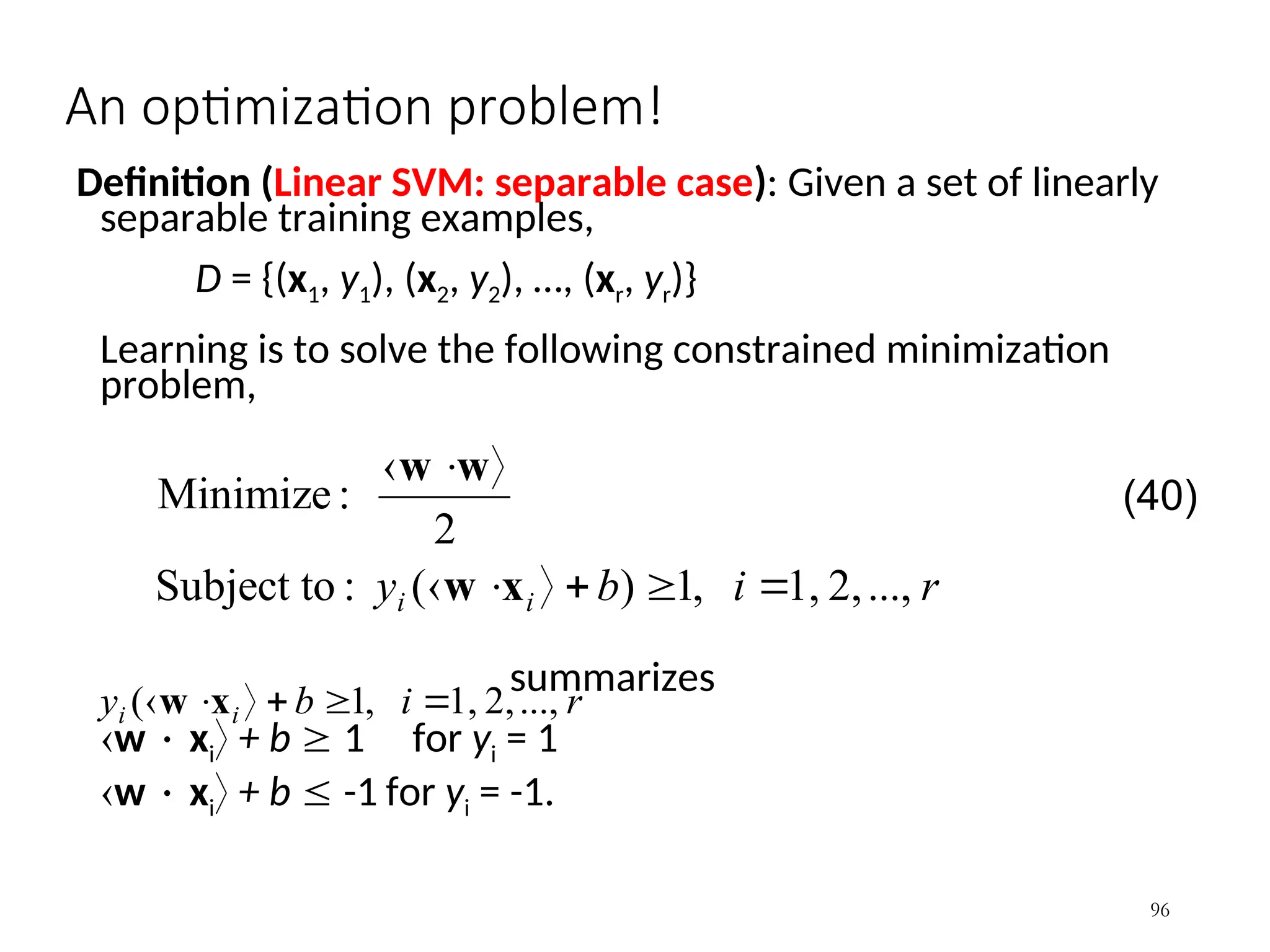
An optimization problem!
Definition(Linear SVM: separable case): Given a set of linearly
separable training examples,
D = {(x1, y1), (x2, y2), …, (xr, yr)}
Learning is to solve the following constrained minimization
problem,
summarizes
w xi + b 1 for yi = 1
w xi + b -1 for yi = -1.
96
r
i
b
y i
i ...,
2,
1,
,
1
)
(
:
Subject to
2
:
Minimize
x
w
w
w
r
i
b
y i
i ...,
2,
1,
,
1
(
x
w
(40)
97.
Solve the constrainedminimization
• Standard Lagrangian method
where i 0 are the Lagrange multipliers.
• Optimization theory says that an optimal solution to (41) must satisfy
certain conditions, called Kuhn-Tucker conditions, which are necessary
(but not sufficient)
• Kuhn-Tucker conditions play a central role in constrained optimization.
97
]
1
)
(
[
2
1
1
b
y
L i
r
i
i
i
P x
w
w
w (41)
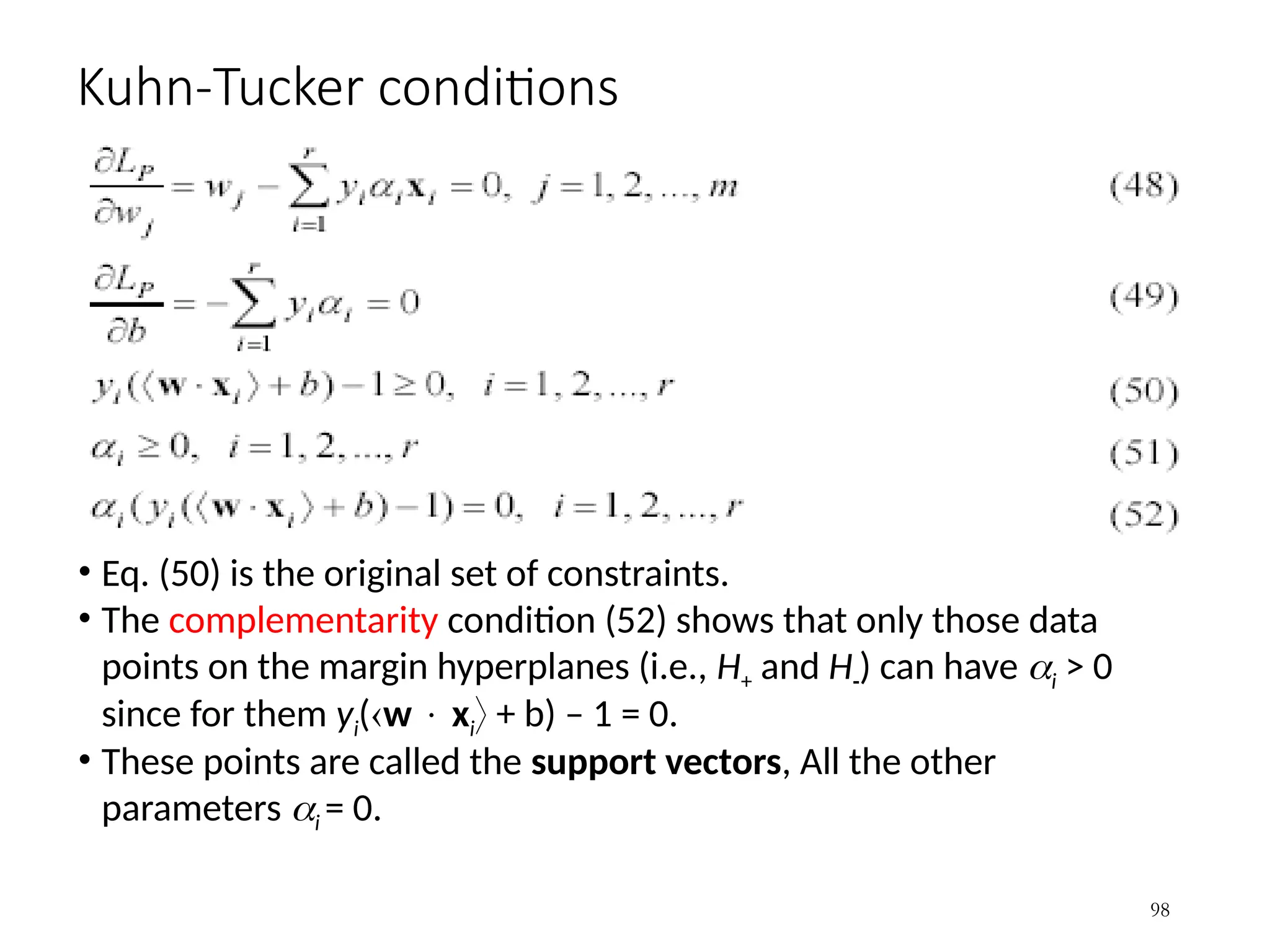
98.
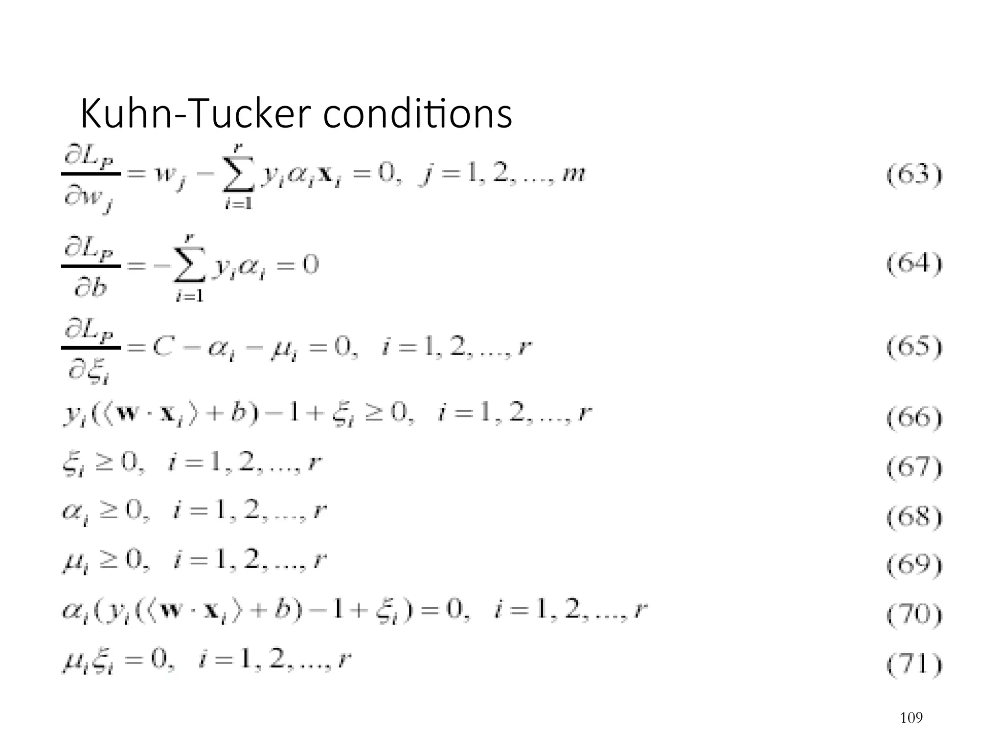
Kuhn-Tucker conditions
• Eq.(50) is the original set of constraints.
• The complementarity condition (52) shows that only those data
points on the margin hyperplanes (i.e., H+ and H-) can have i > 0
since for them yi(w xi + b) – 1 = 0.
• These points are called the support vectors, All the other
parameters i = 0.
98
Solve the problem
•In general, Kuhn-Tucker conditions are necessary for an
optimal solution, but not sufficient.
• However, for our minimization problem with a convex
objective function and linear constraints, the Kuhn-Tucker
conditions are both necessary and sufficient for an
optimal solution.
• Solving the optimization problem is still a difficult task due
to the inequality constraints.
• However, the Lagrangian treatment of the convex
optimization problem leads to an alternative dual
formulation of the problem, which is easier to solve than
the original problem (called the primal).
100
101.
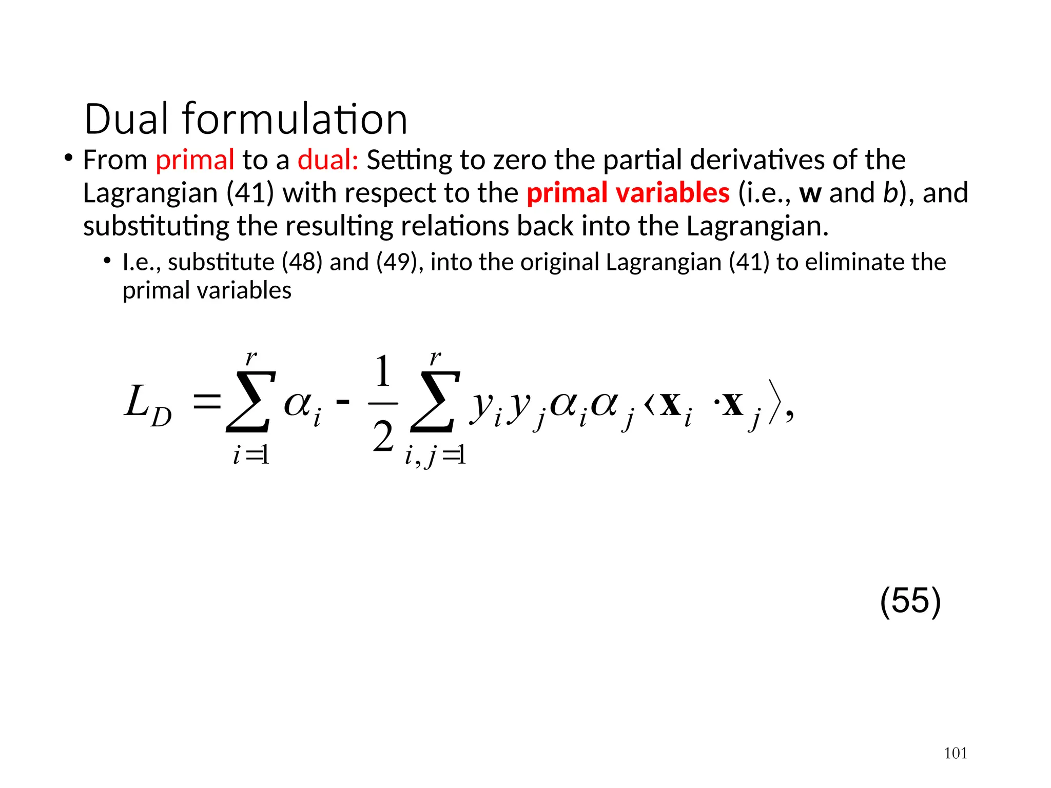
Dual formulation
• Fromprimal to a dual: Setting to zero the partial derivatives of the
Lagrangian (41) with respect to the primal variables (i.e., w and b), and
substituting the resulting relations back into the Lagrangian.
• I.e., substitute (48) and (49), into the original Lagrangian (41) to eliminate the
primal variables
101
(55)
,
2
1
1
,
1
j
i
r
j
i
j
i
j
i
r
i
i
D y
y
L x
x
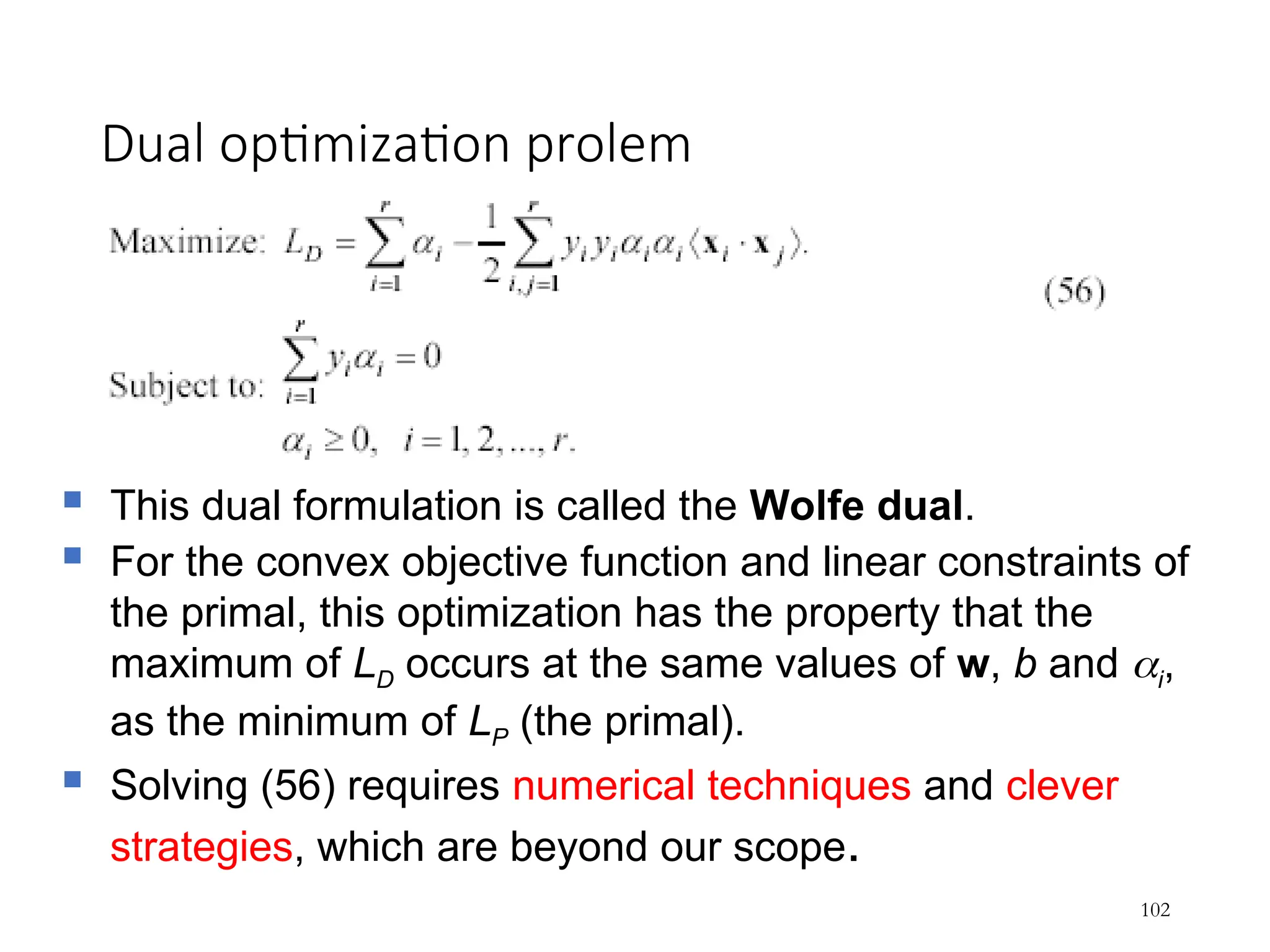
102.
Dual optimization prolem
102
This dual formulation is called the Wolfe dual.
For the convex objective function and linear constraints of
the primal, this optimization has the property that the
maximum of LD occurs at the same values of w, b and i,
as the minimum of LP (the primal).
Solving (56) requires numerical techniques and clever
strategies, which are beyond our scope.
103.
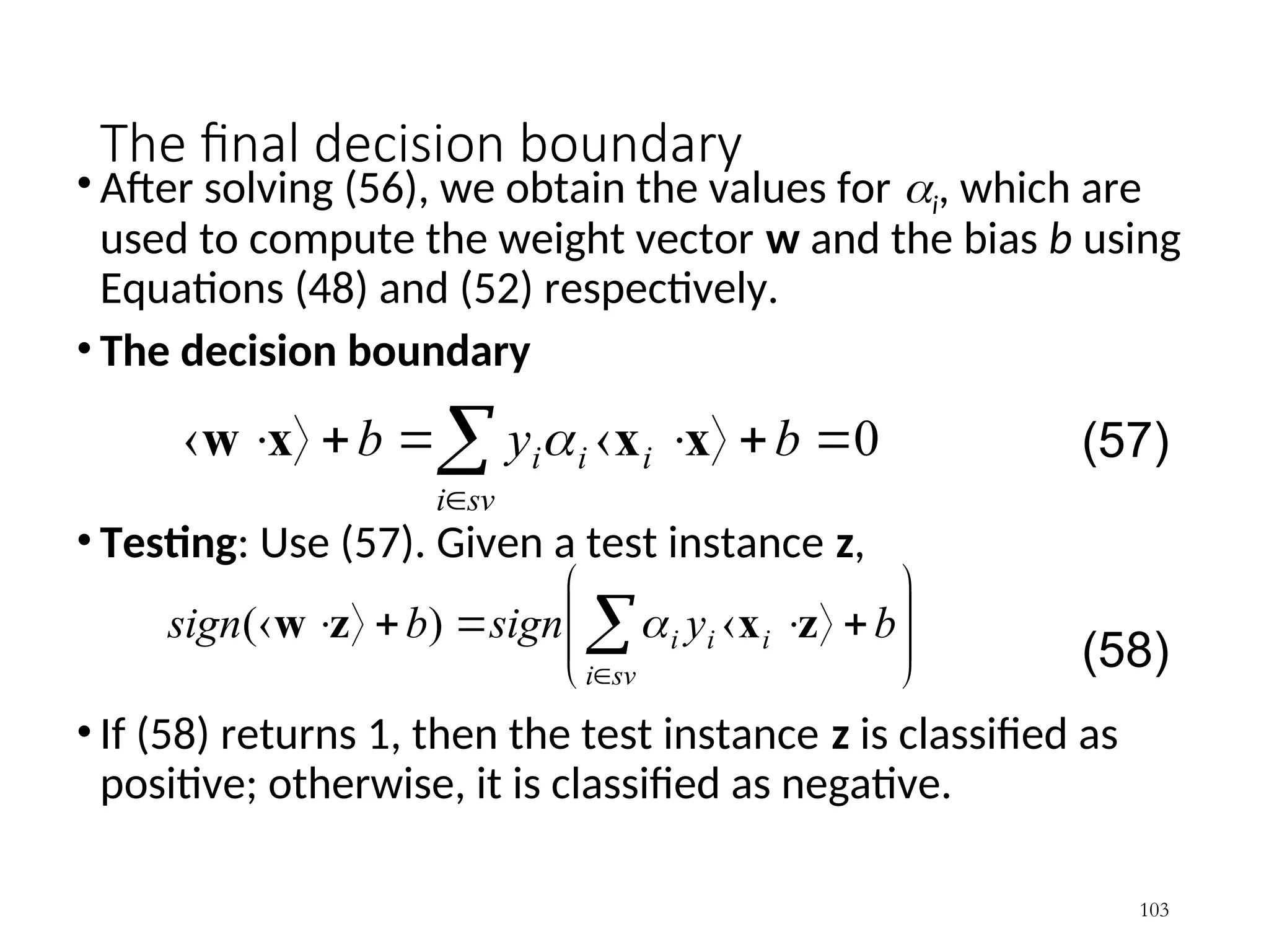
The final decisionboundary
• After solving (56), we obtain the values for i, which are
used to compute the weight vector w and the bias b using
Equations (48) and (52) respectively.
• The decision boundary
• Testing: Use (57). Given a test instance z,
• If (58) returns 1, then the test instance z is classified as
positive; otherwise, it is classified as negative.
103
0
b
y
b
sv
i
i
i
i x
x
x
w (57)
sv
i
i
i
i b
y
sign
b
sign z
x
z
w
)
(
(58)
104.
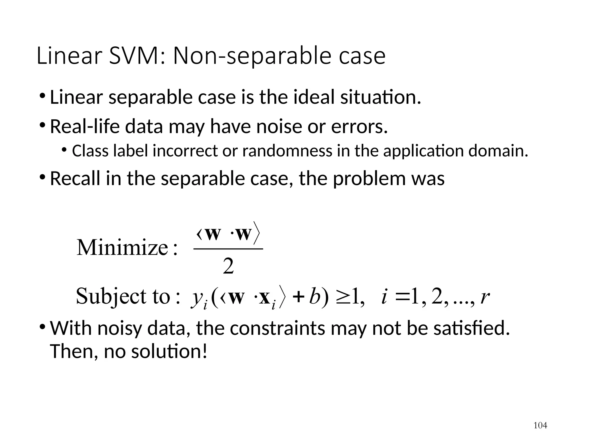
Linear SVM: Non-separablecase
• Linear separable case is the ideal situation.
• Real-life data may have noise or errors.
• Class label incorrect or randomness in the application domain.
• Recall in the separable case, the problem was
• With noisy data, the constraints may not be satisfied.
Then, no solution!
r
i
b
y i
i ...,
2,
1,
,
1
)
(
:
Subject to
2
:
Minimize
x
w
w
w
104
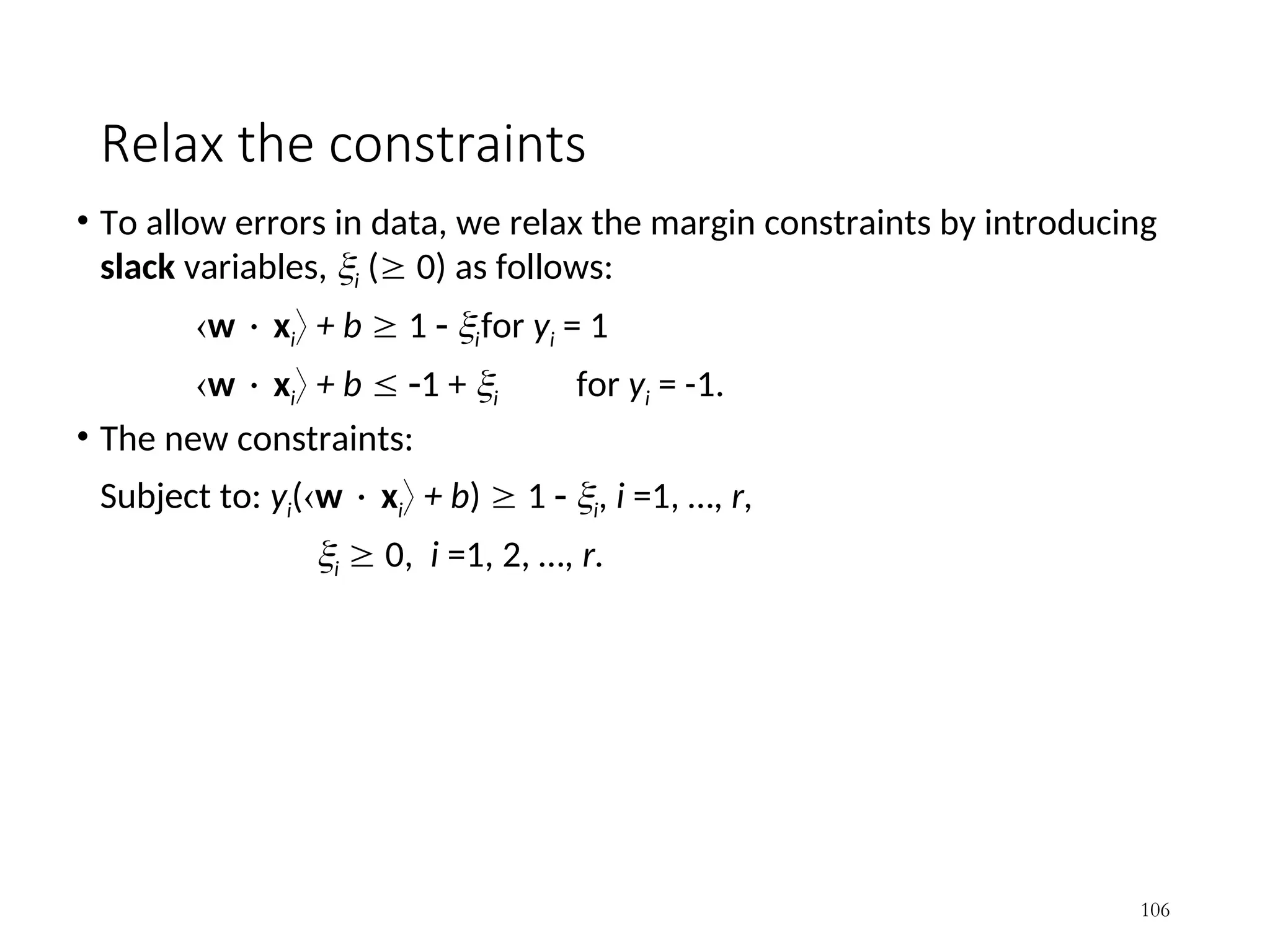
Relax the constraints
•To allow errors in data, we relax the margin constraints by introducing
slack variables, i ( 0) as follows:
w xi + b 1 ifor yi = 1
w xi + b 1 + i for yi = -1.
• The new constraints:
Subject to: yi(w xi + b) 1 i, i =1, …, r,
i 0, i =1, 2, …, r.
106
107.
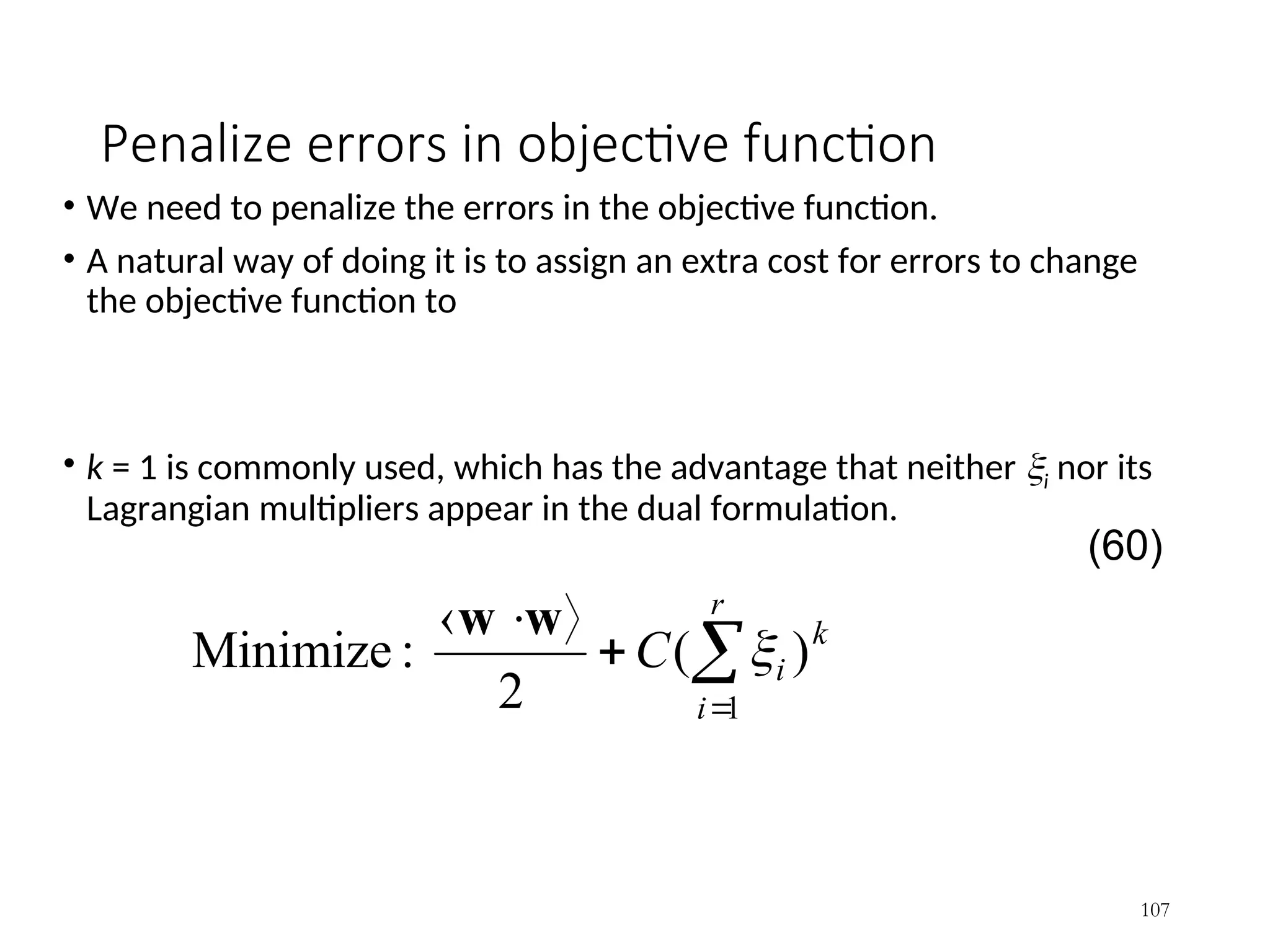
Penalize errors inobjective function
• We need to penalize the errors in the objective function.
• A natural way of doing it is to assign an extra cost for errors to change
the objective function to
• k = 1 is commonly used, which has the advantage that neither i nor its
Lagrangian multipliers appear in the dual formulation.
107
r
i
k
i
C
1
)
(
2
:
Minimize
w
w
(60)
108.
New optimization problem
•This formulation is called the soft-margin SVM. The primal Lagrangian is
where i, i 0 are the Lagrange multipliers
108
r
i
r
i
b
y
C
i
i
i
i
r
i
i
...,
2,
1,
,
0
...,
2,
1,
,
1
)
(
:
Subject to
2
:
Minimize
1
x
w
w
w
(61)
r
i
i
i
i
i
r
i
i
i
r
i
i
P b
y
C
L
1
1
1
]
1
)
(
[
2
1
x
w
w
w
(62)
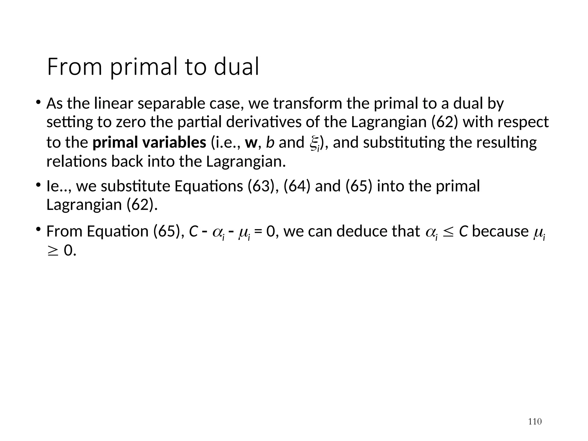
From primal todual
• As the linear separable case, we transform the primal to a dual by
setting to zero the partial derivatives of the Lagrangian (62) with respect
to the primal variables (i.e., w, b and i), and substituting the resulting
relations back into the Lagrangian.
• Ie.., we substitute Equations (63), (64) and (65) into the primal
Lagrangian (62).
• From Equation (65), C i i = 0, we can deduce that i C because i
0.
110
111.
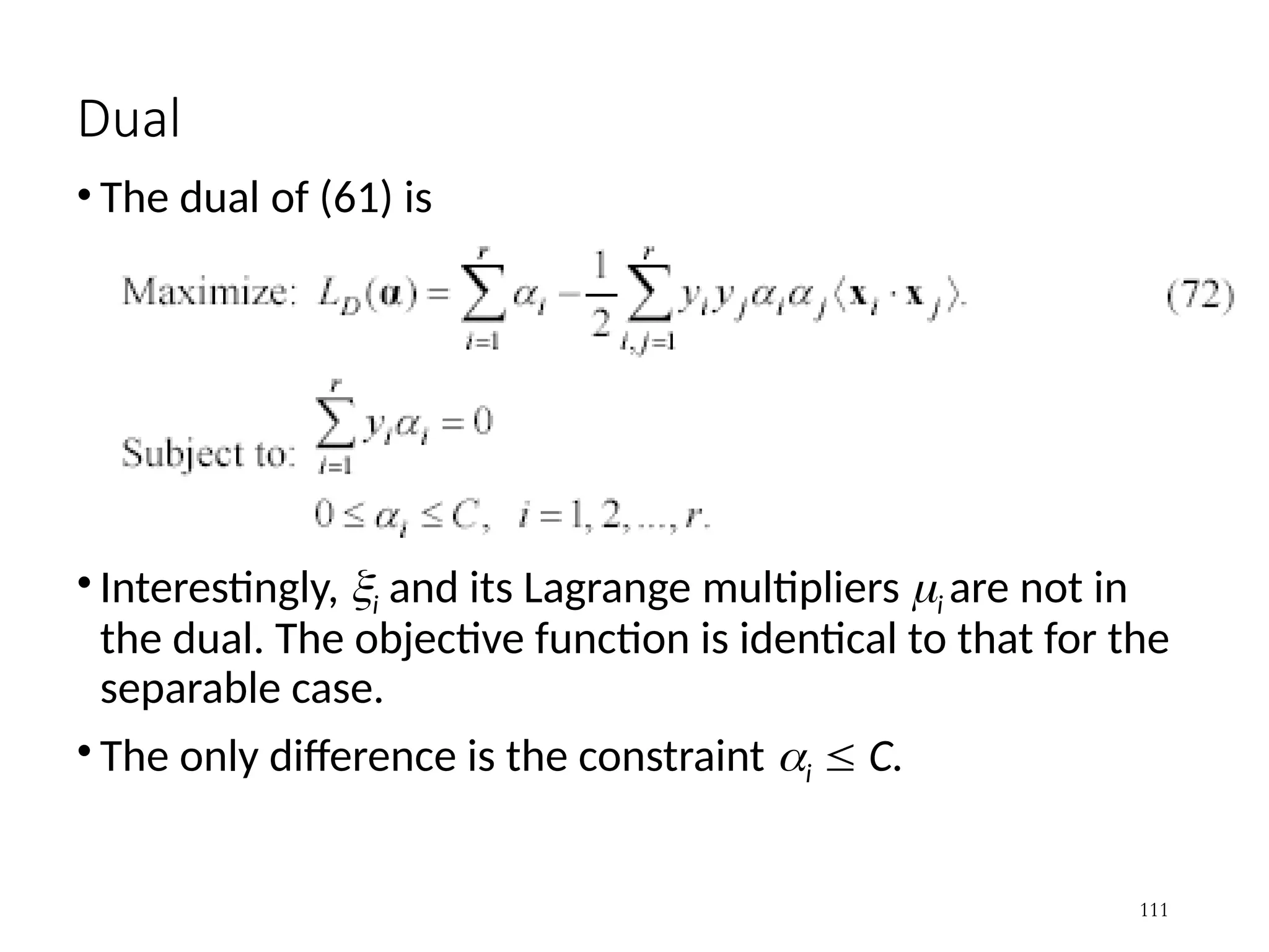
Dual
• The dualof (61) is
• Interestingly, i and its Lagrange multipliers i are not in
the dual. The objective function is identical to that for the
separable case.
• The only difference is the constraint i C.
111
112.
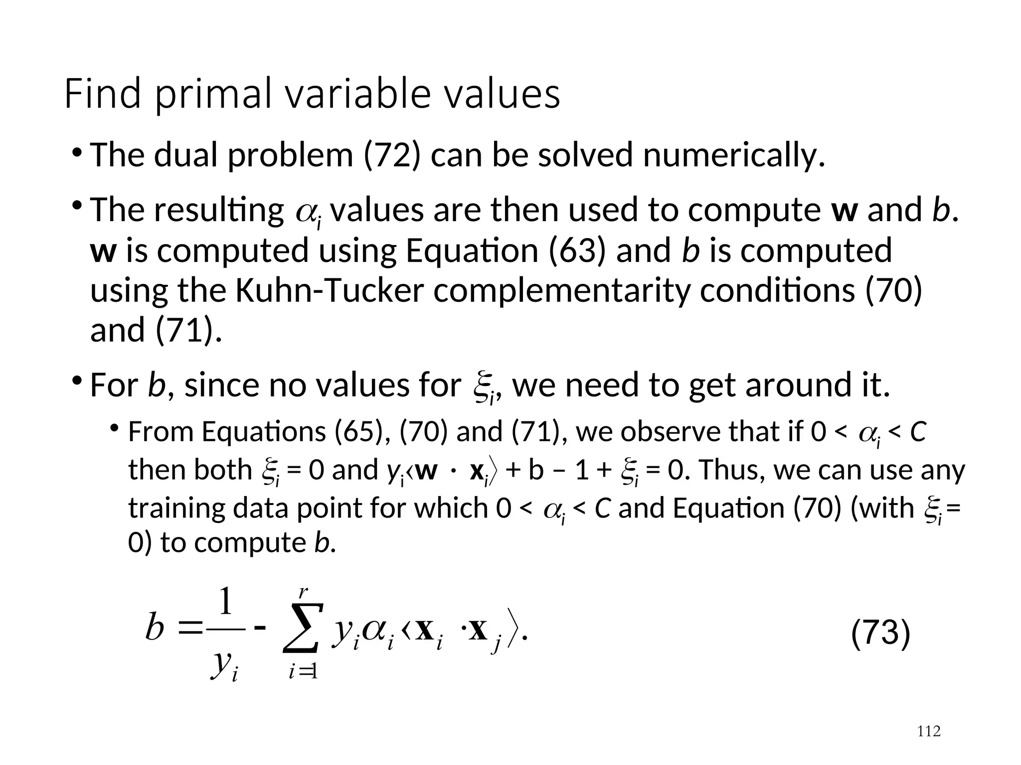
Find primal variablevalues
• The dual problem (72) can be solved numerically.
• The resulting i values are then used to compute w and b.
w is computed using Equation (63) and b is computed
using the Kuhn-Tucker complementarity conditions (70)
and (71).
• For b, since no values for i, we need to get around it.
• From Equations (65), (70) and (71), we observe that if 0 < i < C
then both i = 0 and yiw xi + b – 1 + i = 0. Thus, we can use any
training data point for which 0 < i < C and Equation (70) (with i =
0) to compute b.
112
.
1
1
j
r
i
i
i
i
i
y
y
b x
x
(73)
113.
(65), (70) and(71) in fact tell us more
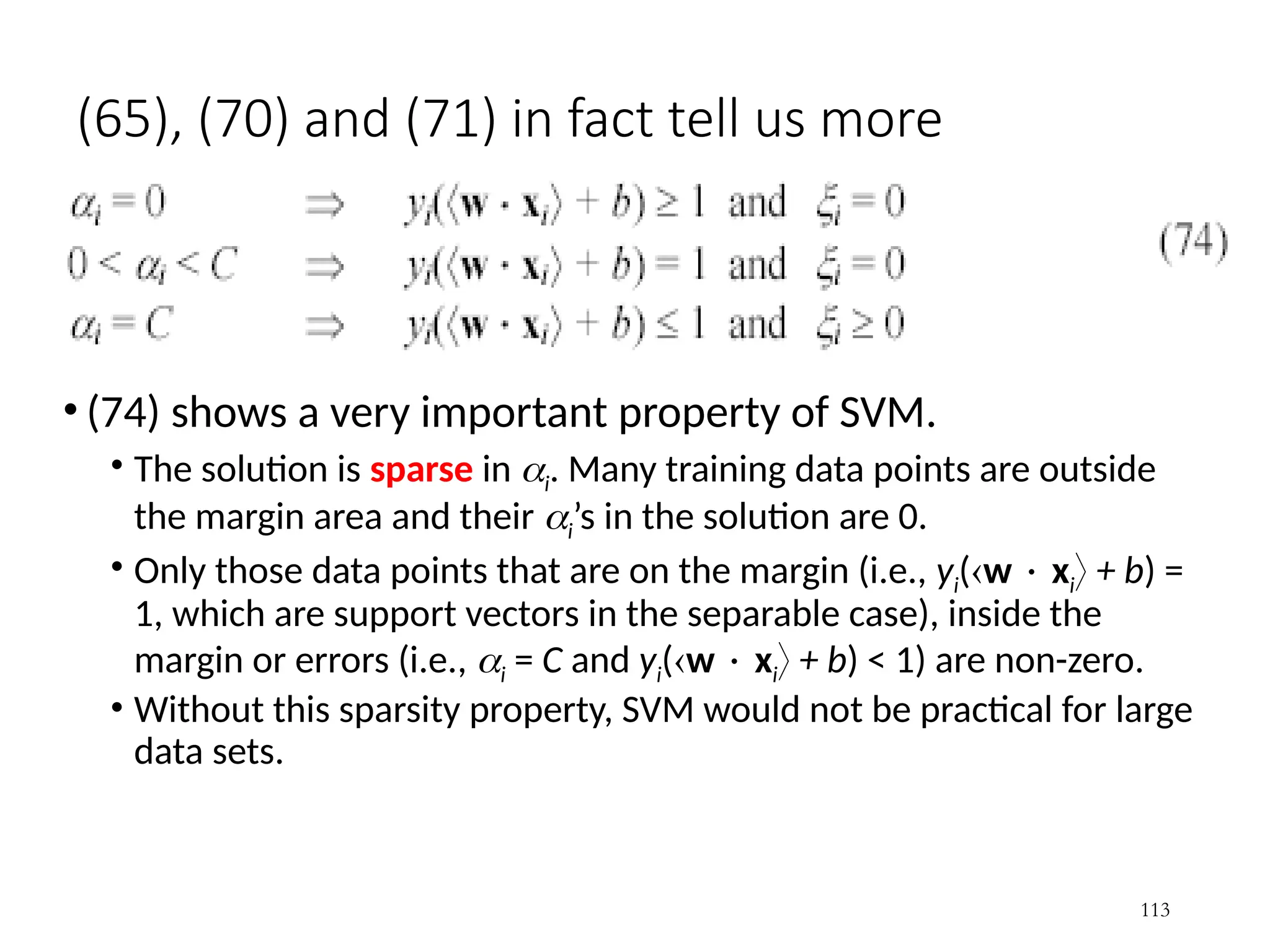
• (74) shows a very important property of SVM.
• The solution is sparse in i. Many training data points are outside
the margin area and their i’s in the solution are 0.
• Only those data points that are on the margin (i.e., yi(w xi + b) =
1, which are support vectors in the separable case), inside the
margin or errors (i.e., i = C and yi(w xi + b) < 1) are non-zero.
• Without this sparsity property, SVM would not be practical for large
data sets.
113
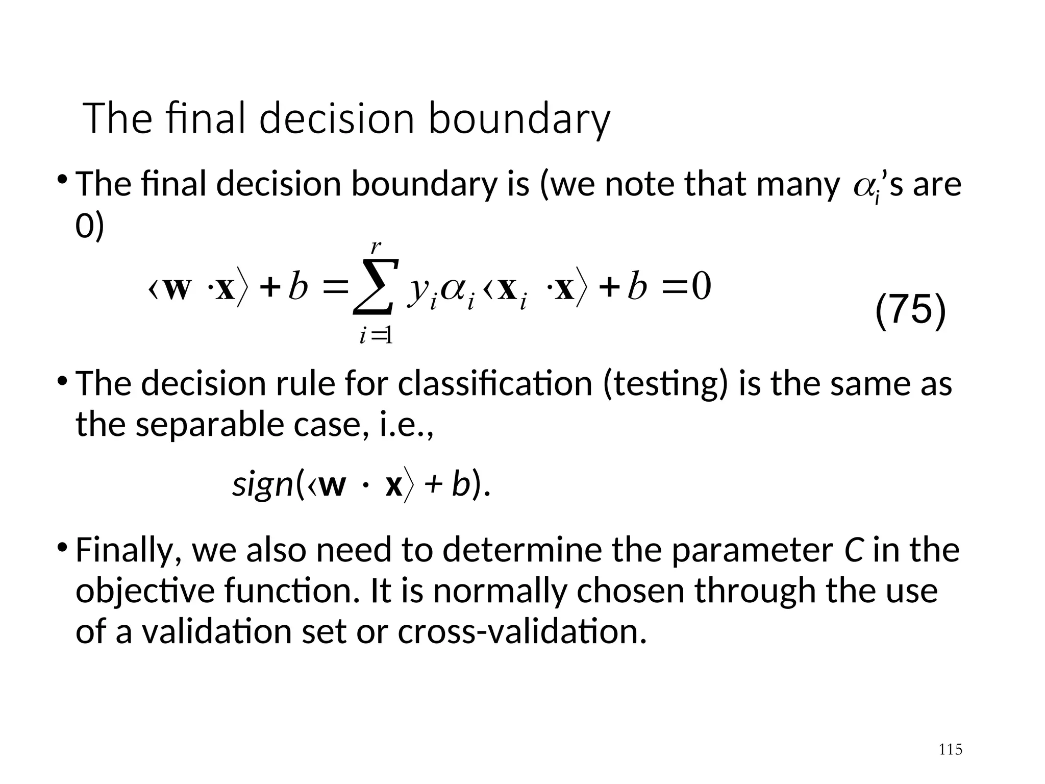
The final decisionboundary
• The final decision boundary is (we note that many i’s are
0)
• The decision rule for classification (testing) is the same as
the separable case, i.e.,
sign(w x + b).
• Finally, we also need to determine the parameter C in the
objective function. It is normally chosen through the use
of a validation set or cross-validation.
115
0
1
b
y
b
r
i
i
i
i x
x
x
w
(75)
116.
How to dealwith nonlinear separation?
• The SVM formulations require linear separation.
• Real-life data sets may need nonlinear separation.
• To deal with nonlinear separation, the same formulation
and techniques as for the linear case are still used.
• We only transform the input data into another space
(usually of a much higher dimension) so that
• a linear decision boundary can separate positive and negative
examples in the transformed space,
• The transformed space is called the feature space. The
original data space is called the input space.
116
117.
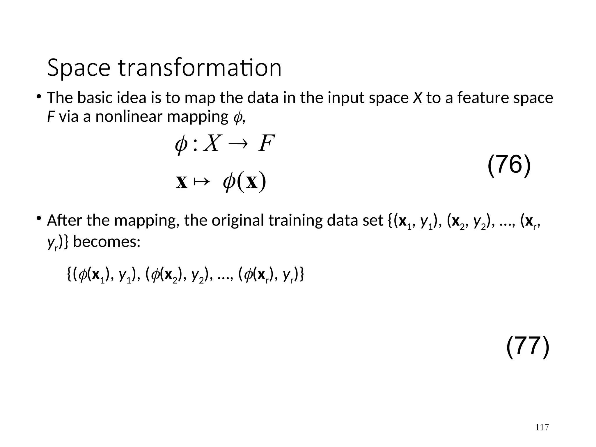
Space transformation
• Thebasic idea is to map the data in the input space X to a feature space
F via a nonlinear mapping ,
• After the mapping, the original training data set {(x1, y1), (x2, y2), …, (xr,
yr)} becomes:
{((x1), y1), ((x2), y2), …, ((xr), yr)}
117
)
(
:
x
x
F
X
(76)
(77)
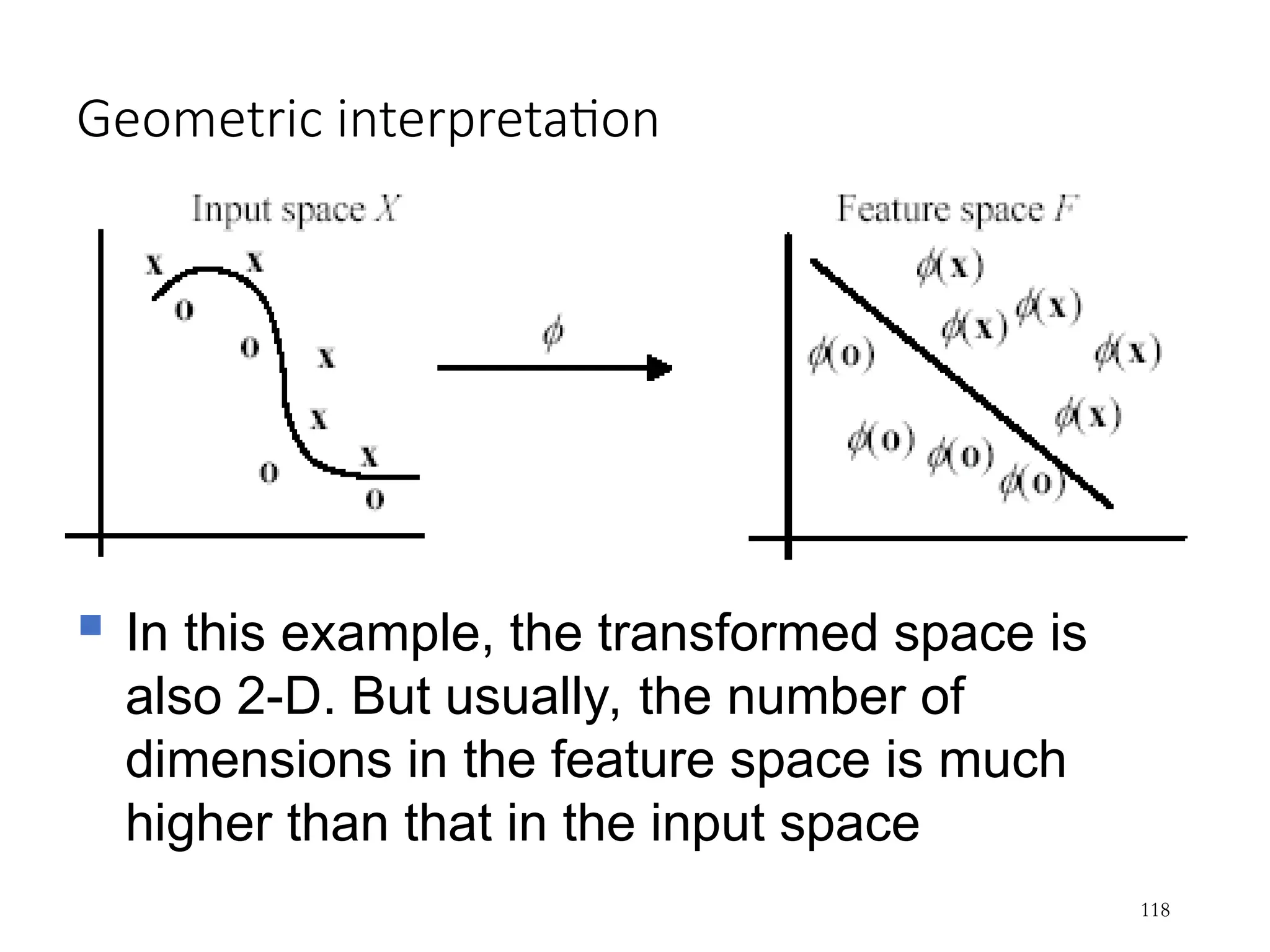
118.
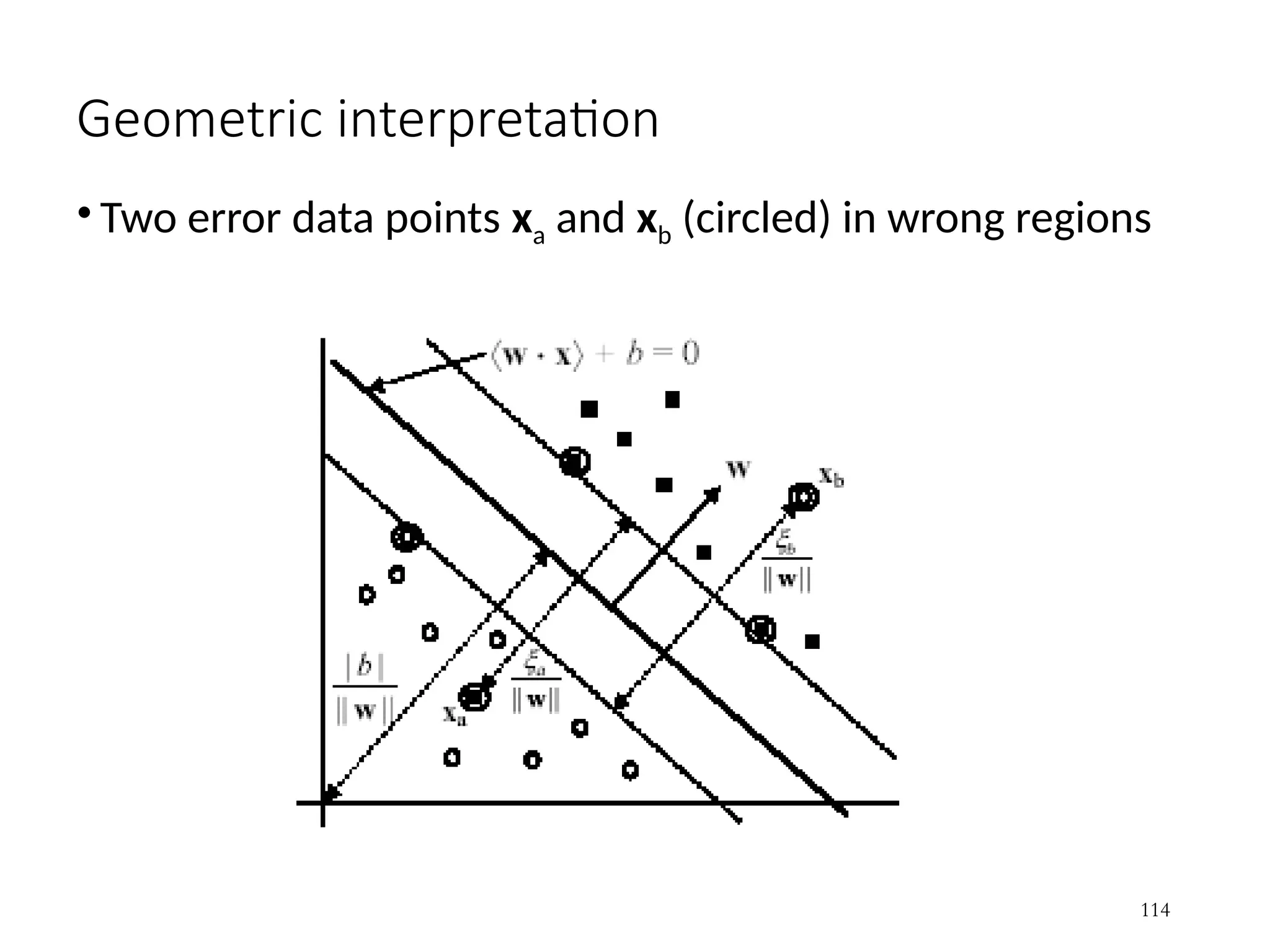
Geometric interpretation
118
Inthis example, the transformed space is
also 2-D. But usually, the number of
dimensions in the feature space is much
higher than that in the input space
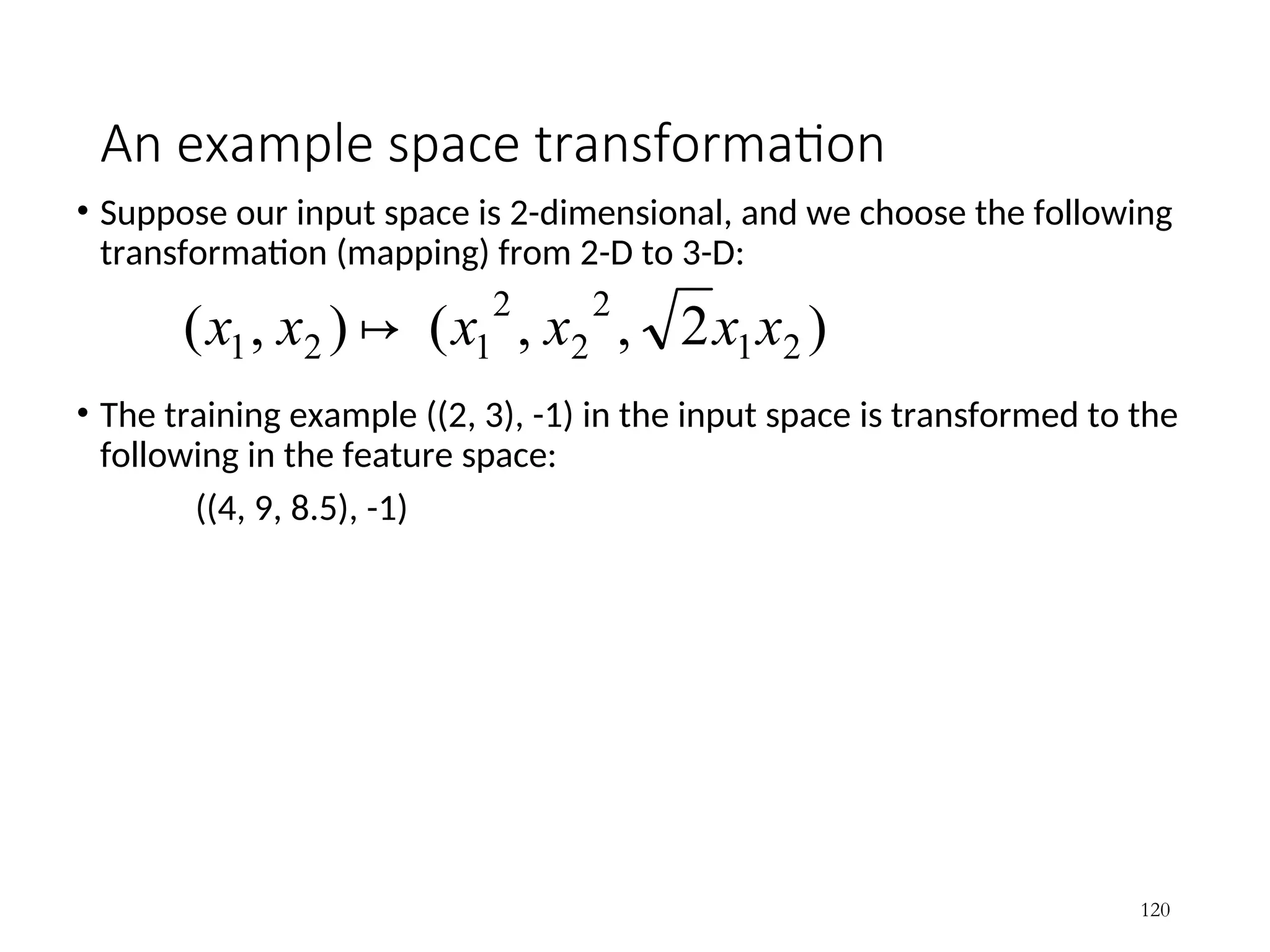
An example spacetransformation
• Suppose our input space is 2-dimensional, and we choose the following
transformation (mapping) from 2-D to 3-D:
• The training example ((2, 3), -1) in the input space is transformed to the
following in the feature space:
((4, 9, 8.5), -1)
120
)
2
,
,
(
)
,
( 2
1
2
2
2
1
2
1 x
x
x
x
x
x
121.
Problem with explicittransformation
• The potential problem with this explicit data
transformation and then applying the linear SVM is that it
may suffer from the curse of dimensionality.
• Huge number of features: The number of dimensions in
the feature space can be huge with some useful
transformations even with reasonable numbers of
attributes in the input space.
• This makes it computationally infeasible to handle.
• Fortunately, explicit transformation is not needed.
121
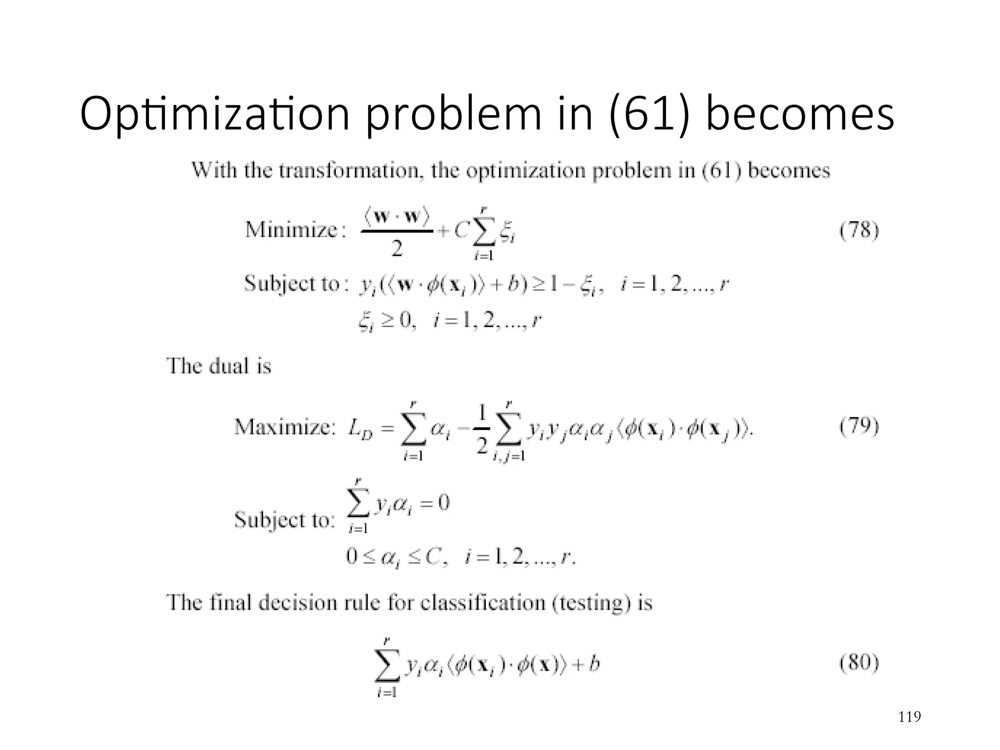
122.
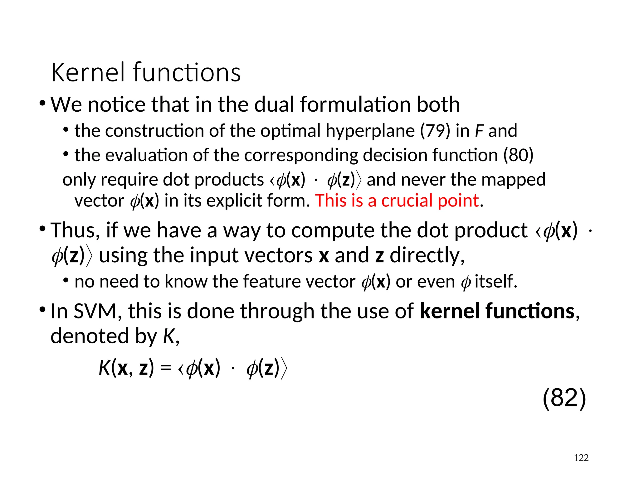
Kernel functions
• Wenotice that in the dual formulation both
• the construction of the optimal hyperplane (79) in F and
• the evaluation of the corresponding decision function (80)
only require dot products (x) (z) and never the mapped
vector (x) in its explicit form. This is a crucial point.
• Thus, if we have a way to compute the dot product (x)
(z) using the input vectors x and z directly,
• no need to know the feature vector (x) or even itself.
• In SVM, this is done through the use of kernel functions,
denoted by K,
K(x, z) = (x) (z)
122
(82)
123.
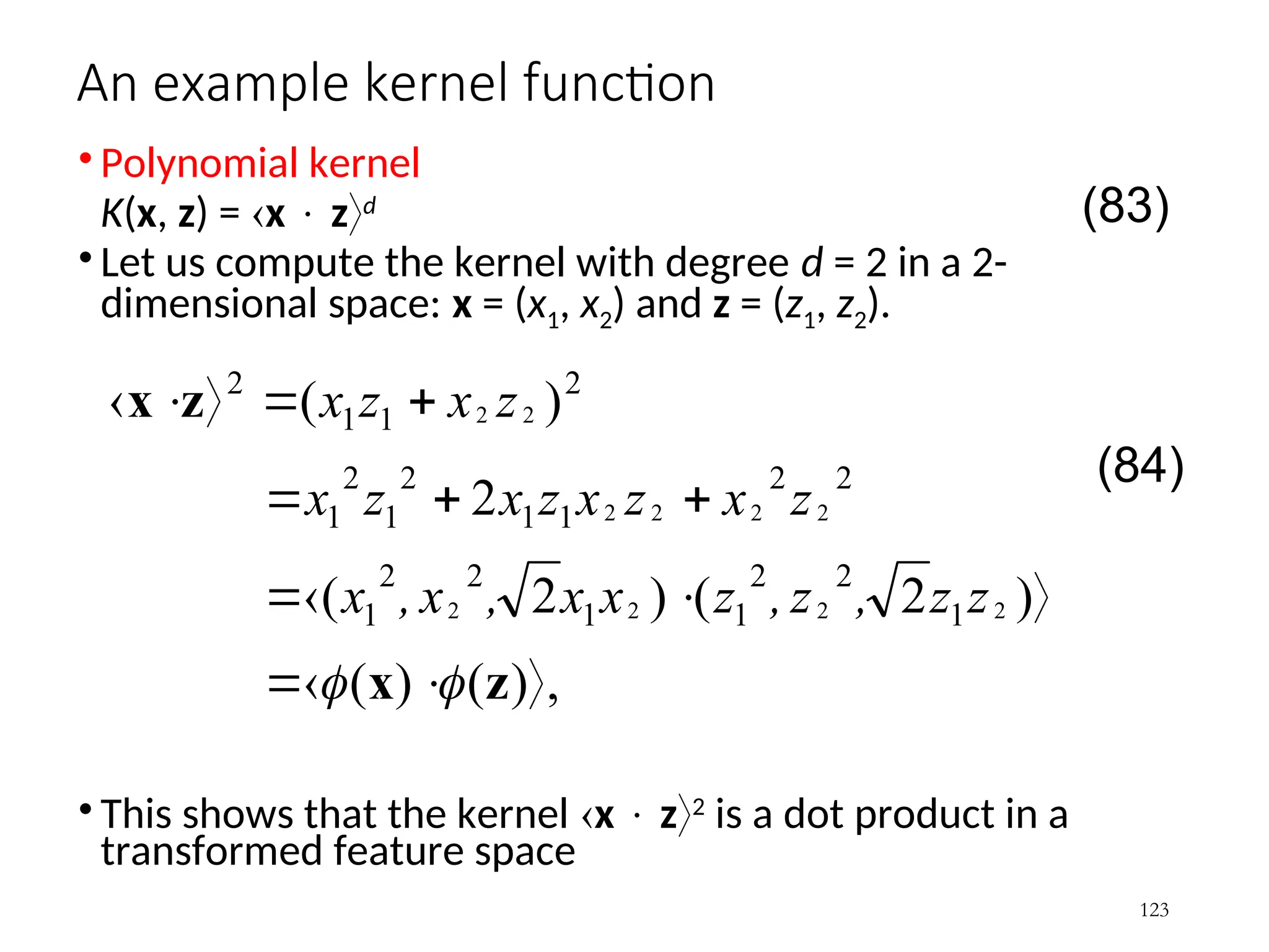
An example kernelfunction
• Polynomial kernel
K(x, z) = x zd
• Let us compute the kernel with degree d = 2 in a 2-
dimensional space: x = (x1, x2) and z = (z1, z2).
• This shows that the kernel x z2
is a dot product in a
transformed feature space
123
(83)
,
)
(
)
(
)
2
(
)
2
(
2
)
(
2
2
2
2
2
2
2
2
2
2
1
2
2
1
1
2
2
1
2
2
1
1
2
1
2
1
2
1
1
2
z
x
z
x
z
z
,
z
,
z
x
x
,
x
,
x
z
x
z
x
z
x
z
x
z
x
z
x
(84)
124.
Kernel trick
• Thederivation in (84) is only for illustration purposes.
• We do not need to find the mapping function.
• We can simply apply the kernel function directly by
• replace all the dot products (x) (z) in (79) and (80) with the kernel function
K(x, z) (e.g., the polynomial kernel x zd
in (83)).
• This strategy is called the kernel trick.
124
125.
Is it akernel function?
• The question is: how do we know whether a function is a kernel without
performing the derivation such as that in (84)? I.e,
• How do we know that a kernel function is indeed a dot product in some feature
space?
• This question is answered by a theorem called the Mercer’s theorem,
which we will not discuss here.
125
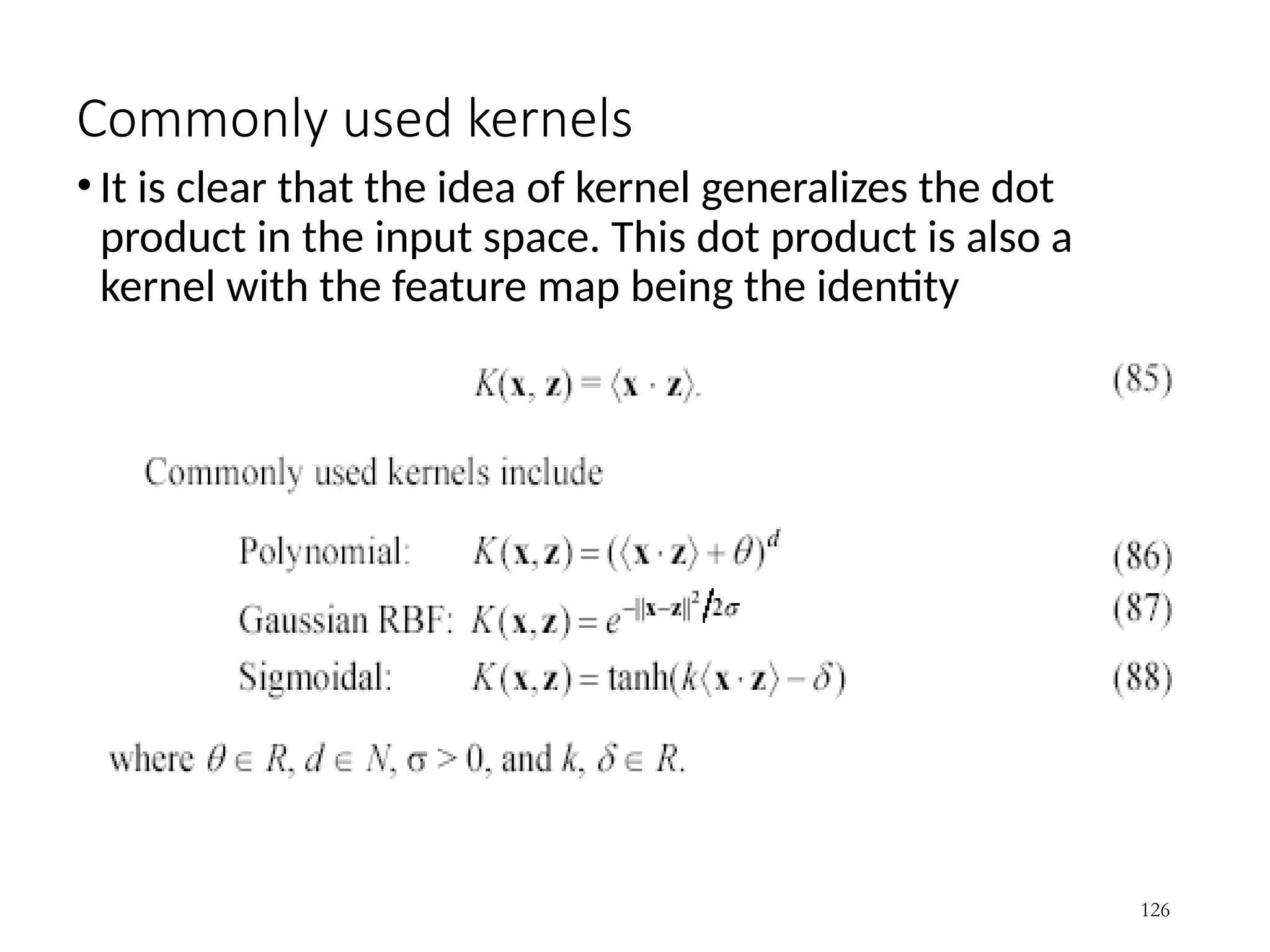
126.
Commonly used kernels
•It is clear that the idea of kernel generalizes the dot
product in the input space. This dot product is also a
kernel with the feature map being the identity
126
127.
Some other issuesin SVM
• SVM works only in a real-valued space. For a categorical
attribute, we need to convert its categorical values to
numeric values.
• SVM does only two-class classification. For multi-class
problems, some strategies can be applied, e.g., one-
against-rest, one-against-one, etc.
• The hyperplane produced by SVM is hard to understand
by human users. The matter is made worse by kernels.
Thus, SVM is commonly used in applications that do not
required human understanding.
127
128.
Road Map
• Basicconcepts
• Decision tree induction
• Evaluation of classifiers
• Naïve Bayesian classification
• Naïve Bayes for text classification
• Support vector machines
• Linear regression and gradient descent
• Neural networks
• K-nearest neighbor
• Ensemble methods
• Summary
128
129.
k-Nearest Neighbor Classification(kNN)
• Unlike all the previous learning methods,
• kNN does not build a model from the training data.
• To classify a test instance t, define k-neighborhood B as k nearest
neighbors of t
• Count number nj of training instances in B that belong to class cj
• Estimate Pr(cj|t) as nj /k
• No training is needed. Classification time is linear in training set size for
each test case.
129
130.
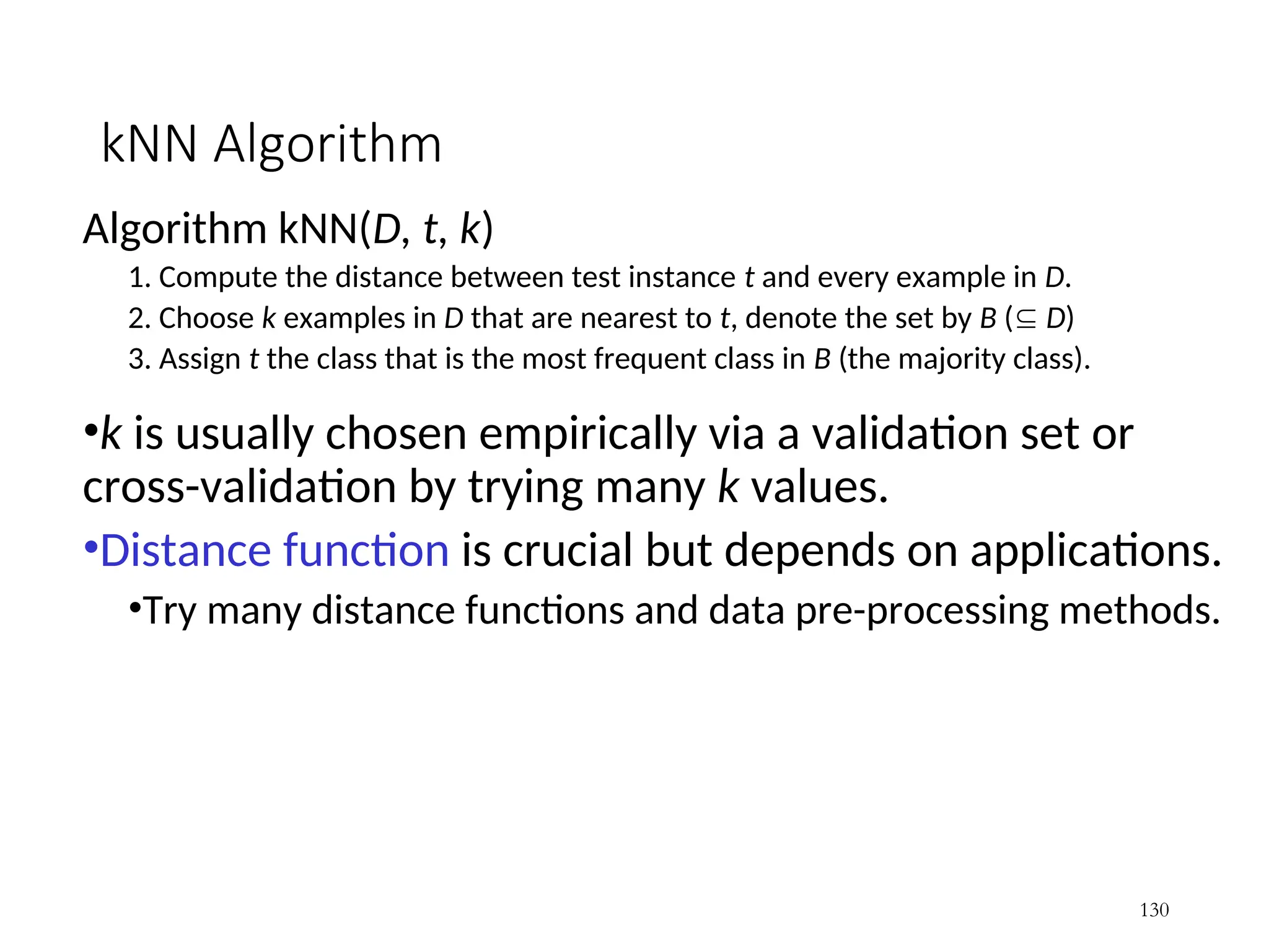
kNN Algorithm
Algorithm kNN(D,t, k)
1. Compute the distance between test instance t and every example in D.
2. Choose k examples in D that are nearest to t, denote the set by B ( D)
3. Assign t the class that is the most frequent class in B (the majority class).
•k is usually chosen empirically via a validation set or
cross-validation by trying many k values.
•Distance function is crucial but depends on applications.
•Try many distance functions and data pre-processing methods.
130
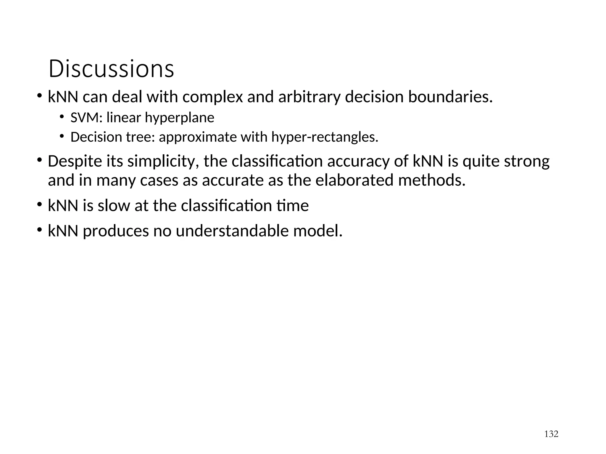
Discussions
• kNN candeal with complex and arbitrary decision boundaries.
• SVM: linear hyperplane
• Decision tree: approximate with hyper-rectangles.
• Despite its simplicity, the classification accuracy of kNN is quite strong
and in many cases as accurate as the elaborated methods.
• kNN is slow at the classification time
• kNN produces no understandable model.
132
133.
Road Map
• Basicconcepts
• Decision tree induction
• Evaluation of classifiers
• Naïve Bayesian classification
• Naïve Bayes for text classification
• Support vector machines
• Linear regression and gradient descent
• Neural networks
• K-nearest neighbor
• Ensemble methods
• Summary
133
134.
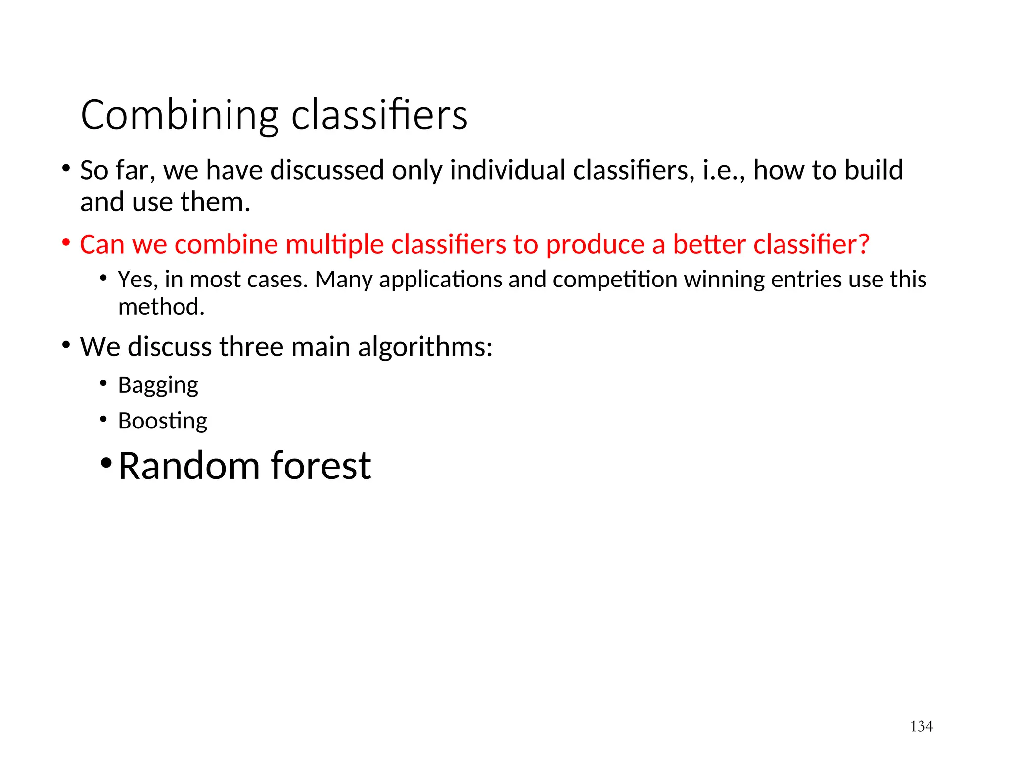
Combining classifiers
• Sofar, we have discussed only individual classifiers, i.e., how to build
and use them.
• Can we combine multiple classifiers to produce a better classifier?
• Yes, in most cases. Many applications and competition winning entries use this
method.
• We discuss three main algorithms:
• Bagging
• Boosting
•Random forest
134
135.
135
Bagging
Breiman, 1996
Bootstrap Aggregating = Bagging
Application of bootstrap sampling
Given: set D containing m training examples
Create a sample S[i] of D by drawing m examples at
random with replacement from D
S[i] of size m: expected to leave out 37% of examples
from D (or (1 - 1/e) ≈ 63.2% unique examples)
136.
136
Bagging (cont…)
Training
Create k bootstrap samples S[1], S[2], …, S[k]
Build a distinct classifier from each S[i] to
produce k classifiers, using the same learning
algorithm.
Testing
Classify each new instance by voting of the k
classifiers (equal weights)
137.
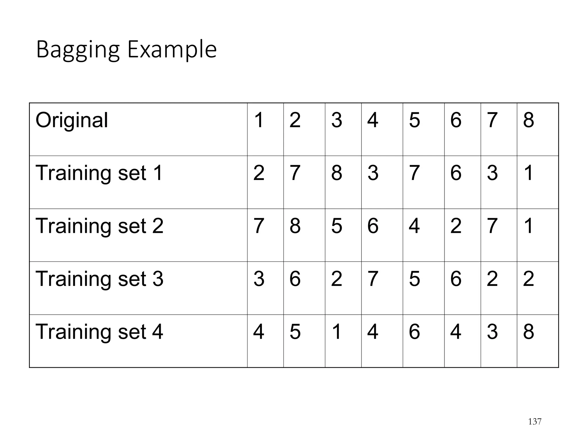
Bagging Example
Original 12 3 4 5 6 7 8
Training set 1 2 7 8 3 7 6 3 1
Training set 2 7 8 5 6 4 2 7 1
Training set 3 3 6 2 7 5 6 2 2
Training set 4 4 5 1 4 6 4 3 8
137
138.
Bagging (cont …)
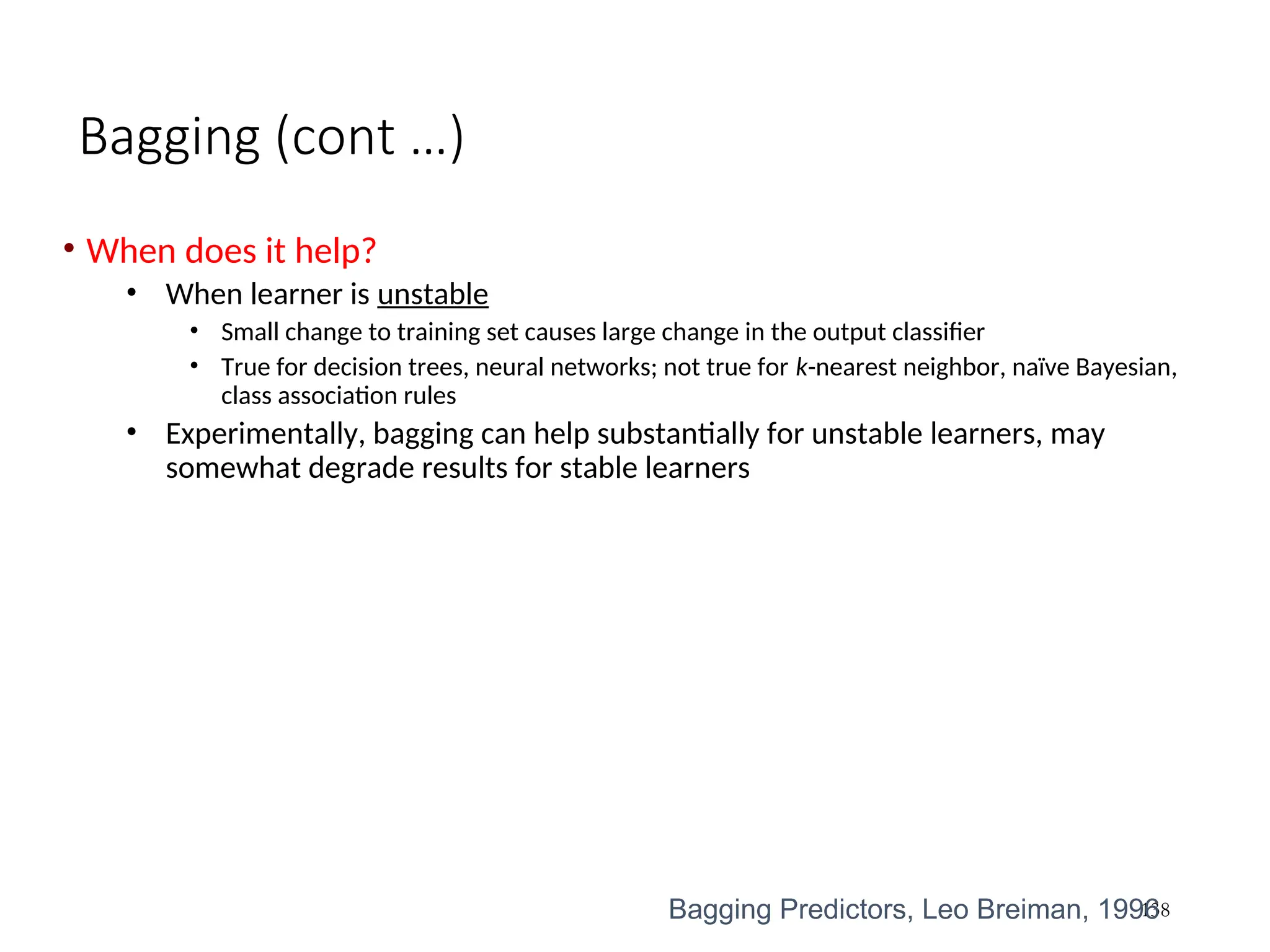
•When does it help?
• When learner is unstable
• Small change to training set causes large change in the output classifier
• True for decision trees, neural networks; not true for k-nearest neighbor, naïve Bayesian,
class association rules
• Experimentally, bagging can help substantially for unstable learners, may
somewhat degrade results for stable learners
138
Bagging Predictors, Leo Breiman, 1996
139.
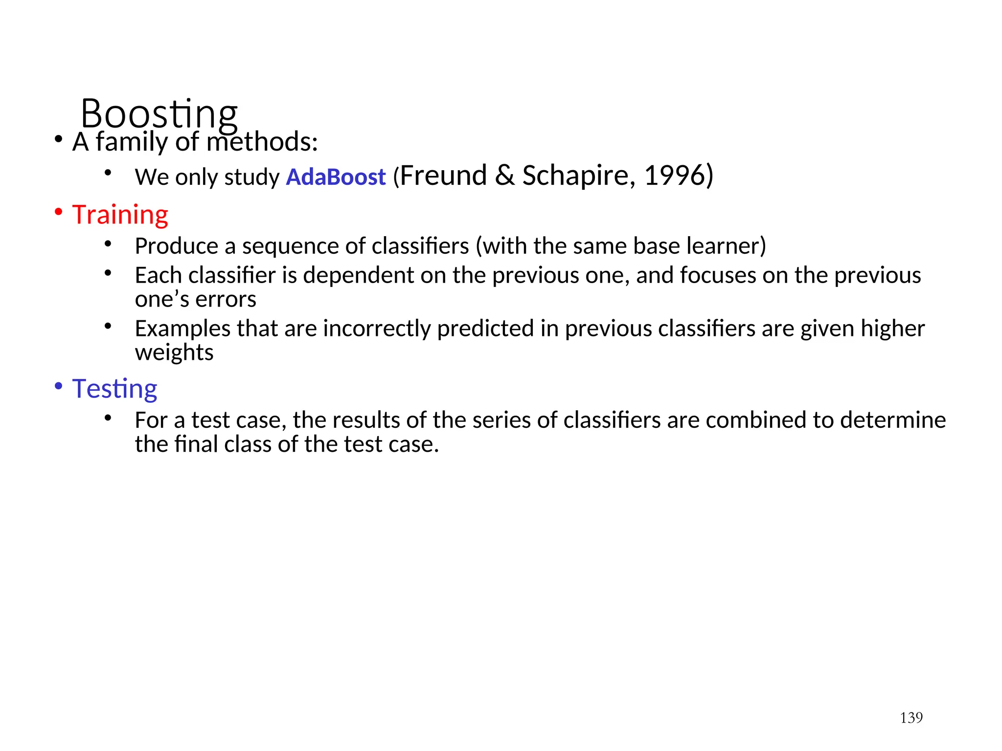
Boosting
• A familyof methods:
• We only study AdaBoost (Freund & Schapire, 1996)
• Training
• Produce a sequence of classifiers (with the same base learner)
• Each classifier is dependent on the previous one, and focuses on the previous
one’s errors
• Examples that are incorrectly predicted in previous classifiers are given higher
weights
• Testing
• For a test case, the results of the series of classifiers are combined to determine
the final class of the test case.
139
140.
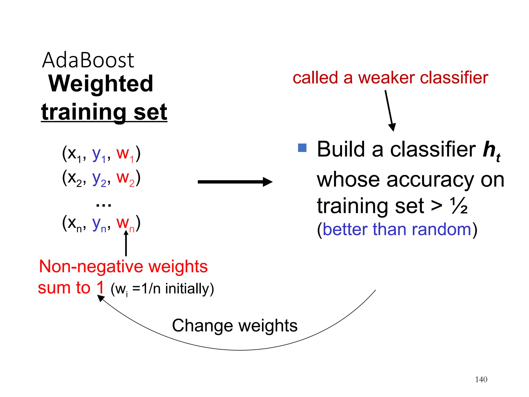
AdaBoost
140
Weighted
training set
(x1, y1,w1)
(x2, y2, w2)
…
(xn, yn, wn)
Non-negative weights
sum to 1 (wi =1/n initially)
Build a classifier ht
whose accuracy on
training set > ½
(better than random)
Change weights
called a weaker classifier
Bagging, Boosting andC4.5
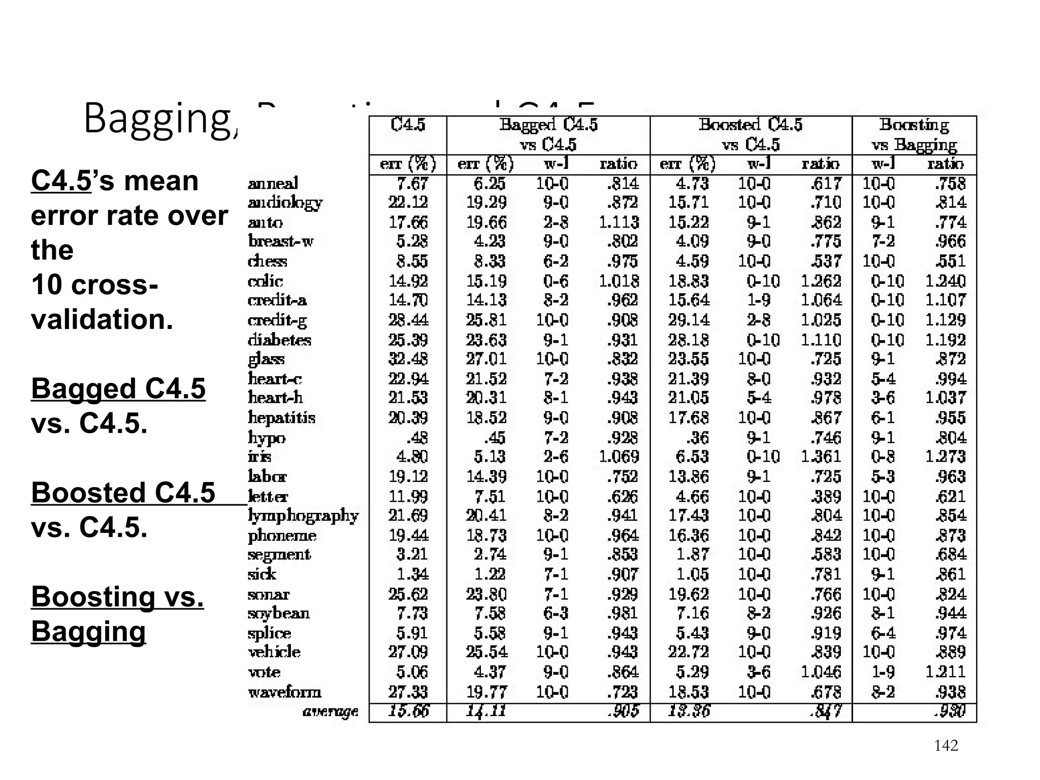
142
C4.5’s mean
error rate over
the
10 cross-
validation.
Bagged C4.5
vs. C4.5.
Boosted C4.5
vs. C4.5.
Boosting vs.
Bagging
143.
Does AdaBoost alwayswork?
• The actual performance of boosting depends on the data and the base
learner.
• It requires the base learner to be unstable as bagging.
• Boosting seems to be susceptible to noise.
• When the number of outliners is very large, the emphasis placed on the hard
examples can hurt the performance.
143
144.
Random forest
•Based ondecision tree: probably the most effective
classification ensemble in general.
•First proposed by Tin Kam Ho (1995). “Random
Decision Forests.” Proceedings of the 3rd International
Conference on Document Analysis and Recognition.
• Random trees: randomly sample a subset of attributes at
each node.
•Improved by Leo Breiman (2001). "Random
Forests". Machine Learning. 45(1): 5–32.
• Combining Random Decision Forests with Bagging
144
145.
Random forest algorithm
Training
•fori = 1 … T
• Draw a bootstrap sample S[i] of D like bagging.
• Build a random-forest tree using S[i]
• For a node j, sample a random subset k (= sqrt(|Ai|)) of the attributes Ai remaining at the
node.
• Select the best attribute from k attributes to split the tree
•end-for
Testing: voting like bagging.
145
146.
Road Map
• Basicconcepts
• Decision tree induction
• Evaluation of classifiers
• Naïve Bayesian classification
• Naïve Bayes for text classification
• Support vector machines
• Linear regression and gradient descent
• Neural networks
• K-nearest neighbor
• Ensemble methods
• Summary
146
147.
Summary
• Supervised learning(SL) applications: everywhere.
• We studied 8 techniques, but there are many more:
• E.g., Bayesian networks, genetic algorithms, fuzzy classification,
and (More importantly) neural networks.
• This large number of methods show the importance of SL or
classification.
• There are many other old and new topics in SL, e.g.,
• Classic topics: transfer learning, multi-task learning, one-class
learning, semi-supervised learning, online learning, active
learning, etc.
• New topics: Lifelong and continual learning, open-world learning,
out-of-distribution, etc.
147
Editor's Notes
#6 Induction is different from deduction and DBMS does not not support induction;
The result of induction is higher-level information or knowledge: general statements about data
There are many approaches. Refer to the lecture notes for CS3244 available at the Co-Op.
We focus on three approaches here, other examples:
Other approaches
Instance-based learning
other neural networks
Concept learning (Version space, Focus, Aq11, …)
Genetic algorithms
Reinforcement learning


![Solve the constrained minimization
• Standard Lagrangian method
where i 0 are the Lagrange multipliers.
• Optimization theory says that an optimal solution to (41) must satisfy
certain conditions, called Kuhn-Tucker conditions, which are necessary
(but not sufficient)
• Kuhn-Tucker conditions play a central role in constrained optimization.
97
]
1
)
(
[
2
1
1
b
y
L i
r
i
i
i
P x
w
w
w (41)](https://image.slidesharecdn.com/msc-dfis-17-supervised-learning-250306010909-5e7981f5/75/MSC-DFIS-17-supervised-learning-Algorithms-ppt-97-2048.jpg)

![New optimization problem
• This formulation is called the soft-margin SVM. The primal Lagrangian is
where i, i 0 are the Lagrange multipliers
108
r
i
r
i
b
y
C
i
i
i
i
r
i
i
...,
2,
1,
,
0
...,
2,
1,
,
1
)
(
:
Subject to
2
:
Minimize
1
x
w
w
w
(61)
r
i
i
i
i
i
r
i
i
i
r
i
i
P b
y
C
L
1
1
1
]
1
)
(
[
2
1
x
w
w
w
(62)](https://image.slidesharecdn.com/msc-dfis-17-supervised-learning-250306010909-5e7981f5/75/MSC-DFIS-17-supervised-learning-Algorithms-ppt-108-2048.jpg)

![135
Bagging
Breiman, 1996
Bootstrap Aggregating = Bagging
Application of bootstrap sampling
Given: set D containing m training examples
Create a sample S[i] of D by drawing m examples at
random with replacement from D
S[i] of size m: expected to leave out 37% of examples
from D (or (1 - 1/e) ≈ 63.2% unique examples)](https://image.slidesharecdn.com/msc-dfis-17-supervised-learning-250306010909-5e7981f5/75/MSC-DFIS-17-supervised-learning-Algorithms-ppt-135-2048.jpg)
![136
Bagging (cont…)
Training
Create k bootstrap samples S[1], S[2], …, S[k]
Build a distinct classifier from each S[i] to
produce k classifiers, using the same learning
algorithm.
Testing
Classify each new instance by voting of the k
classifiers (equal weights)](https://image.slidesharecdn.com/msc-dfis-17-supervised-learning-250306010909-5e7981f5/75/MSC-DFIS-17-supervised-learning-Algorithms-ppt-136-2048.jpg)
![Random forest algorithm
Training
•for i = 1 … T
• Draw a bootstrap sample S[i] of D like bagging.
• Build a random-forest tree using S[i]
• For a node j, sample a random subset k (= sqrt(|Ai|)) of the attributes Ai remaining at the
node.
• Select the best attribute from k attributes to split the tree
•end-for
Testing: voting like bagging.
145](https://image.slidesharecdn.com/msc-dfis-17-supervised-learning-250306010909-5e7981f5/75/MSC-DFIS-17-supervised-learning-Algorithms-ppt-145-2048.jpg)


![[DSC Europe 25] Vid Stimac - Policy Parsimony: Between Oversimplifying and Ov...](https://cdn.slidesharecdn.com/ss_thumbnails/eqlepagzqp2rhg3gbluh-dsc-stimac-251120-251205090438-059e7f54-thumbnail.jpg?width=640&height=640&fit=bounds)

![[DSC Europe 25] Andy Cotgreave - Nothing is new in analytics.pptx](https://cdn.slidesharecdn.com/ss_thumbnails/mba4vzcurvoh5lfrd5zw-6-251205194645-341bbbbe-thumbnail.jpg?width=640&height=640&fit=bounds)
![[DSC Europe 25] Jim Sterne - Adopting Generative AI Capabilities Into the Ent...](https://cdn.slidesharecdn.com/ss_thumbnails/sxhpofuorcagxsaulkmt-3-251204082258-7e66bc48-thumbnail.jpg?width=640&height=640&fit=bounds)

![[DSC Europe 25] Yemi Olagbaiye - From Senses to Systems: Building Organisatio...](https://cdn.slidesharecdn.com/ss_thumbnails/zhgiesqoqd68z6lkos3o-5-251203092157-dcce0c99-thumbnail.jpg?width=640&height=640&fit=bounds)
![[DSC Europe 25] Bogdan Daniel Maruneac - AI - It starts with you.pptx](https://cdn.slidesharecdn.com/ss_thumbnails/odov3snhrcqs9hx5ny2n-4-251205085715-f1daacfe-thumbnail.jpg?width=640&height=640&fit=bounds)

![[DSC Europe 25] Dusan Jovicic - AI Story: From on-prem to cloud and back agai...](https://cdn.slidesharecdn.com/ss_thumbnails/8kp49m6uq22ifnbwhfnk-2-251205085715-964d11a6-thumbnail.jpg?width=640&height=640&fit=bounds)


![[DSC Europe 25] Max Talanov - Non digital NNs.pptx](https://cdn.slidesharecdn.com/ss_thumbnails/wif8tr3gtua74qvtopke-non-digital-nns-251205090438-26b0eea6-thumbnail.jpg?width=640&height=640&fit=bounds)


