Image Denoising by using Modified SGHP Algorithm

International Journal of Electrical and Computer Engineering (IJECE)
Vol. 8, No. 2, April 2018, pp. 971~978
ISSN: 2088-8708, DOI: 10.11591/ijece.v8i1.pp971-978  971
Journal homepage: http://iaescore.com/journals/index.php/IJECE
Image Denoising by using Modified SGHP Algorithm
Sreedhar Kollem1
, K. Ramalinga Reddy2
, D. Sreenivasa Rao3
1
Department of Electronics and Communication Engineering, SR Engineering College, Warangal, Telangana, India
2
Department of Electronics and Telematics Engineering,
G. Narayanamma Institute of Technology and Science Hyderabad, Telangana, India
3
Department of Electronics and Communication Engineering, JNTUH CEH, Kukatpally, Hyderabad, Telangana, India
Article Info ABSTRACT
Article history:
Received Sep 20, 2017
Revised Dec 27, 2017
Accepted Jan 7, 2018
In real time applications, image denoising is a predominant task. This task
makes adequate preparation for images looks prominent. But there are
several denoising algorithms and every algorithm has its own distinctive
attribute based upon different natural images. In this paper, we proposed a
perspective that is modified parameter in S-Gradient Histogram Preservation
denoising method. S-Gradient Histogram Preservation is a method to
compute the structure gradient histogram from the noisy observation by
taking different noise standard deviations of different images. The
performance of this method is enumerated in terms of peak signal to noise
ratio and structural similarity index of a particular image. In this paper,
mainly focus on peak signal to noise ratio, structural similarity index, noise
estimation and a measure of structure gradient histogram of a given image.
Keyword:
Gradient histogram
Noise estimation
Principal component analysis
PSNR
S-GHP
SSIM
Copyright © 2018 Institute of Advanced Engineering and Science.
All rights reserved.
Corresponding Author:
Sreedhar Kollem
Department of Electronics and Communication Engineering,
SR Engineering College,
Warangal, Telangana, India.
Email: ksreedhar446@gmail.com
1. INTRODUCTION
Images affected by unwanted noise from different sources like traditional film cameras and digital
cameras. These noise elements will create some serious issues for further processing of images in practical
applications such as computer vision, artistic work or marketing and also in many fields. So, different
classification of noises likes salt and pepper, Gaussian, shot and quantization. In salt and pepper noise, all the
images are constructed with pixels in a two-dimensional array. In that pixel to pixel, the difference is
observed when the image is affected by noise that is in terms of intensity of neighbouring pixels. So, it is
identified pixels and neighbouring pixels only the small number of pixels is affected in an image. The salt
and pepper noise is clearly identified in an image by it contains black and white speckles. When we viewed
an image which is affected by salt and pepper noise, the image contains black and white dots, hence it terms
as salt and pepper noise.
In Gaussian noise, noisy pixel value will be a small change of the original value of a pixel. A
diagram consisting of rectangles whose area is proportional to the frequency of a variable or PSNR and
whose width is equal to the different noise standard deviations is a histogram. Other Gaussian models are
present mainly depends upon the central limit theorem shows that addition of different noises from different
sources to associated with Gaussian distribution.
Denoising of an image involves the manipulation of the image data to produce a visually high-
quality image. There are numerous models that have been published so far which are used for denoising an
image [1]. Sparse representation for image restoration [2], [3], Total variation model [4], Wavelet-based
model [5], BM3D [6] model and histogram preservation algorithm [7] are some of them. Each method has its
own characteristics, benefit and also demerit. Two major classes of denoising methods are (a) model based

 ISSN: 2088-8708
Int J Elec & Comp Eng, Vol. 8, No. 2, April 2018 : 971 – 978
972
and (b) Learning-based method. In the model, based method, a statistical/mathematical model will be used
for the denoising. Whereas in Learning based method, an algorithm will be trained by using sufficient
parameters and then the model is allowed to work based on its weightage function [8].
2. PROPOSED METHOD
In the present work, the denoising is done in a more realistic way as in practical situations, only the
noisy image will be available. A noisy image is taken as input to the algorithm is shown in Figure 1. We have
adopted patch-based noise level estimation algorithm by Xinhao Liu et al [9]. Patches are generated from the
single noisy image and its weak textured patches are identified. The Noise level is estimated from the
Principal Component Analysis [10], [11].
Figure 1. Flowchart of the proposed algorithm
In most of the denoising method, it is seen that, after its implementation, the image will be blurred
than that of the original image. Also, the edge of the denoised image gets smoothened and will have lesser
details than that of the original image. A study has been conducted to find the edge of the original and noisy
image by using sample data. In this study, it is found that there fewer details of edges in the denoised image.
To address this issue, we have employed fuzzy based edge detection and then the edge is enhanced in the
denoised image that we have received by using our method. Now the denoising is performed based on the
modified parameter S-GHP focus on smoothing of the image by implementing the gradient histogram
preservation.
2.1. Noise estimation
Input image is decomposed into overlapping patches by
y z ni i i  (1)
Where zi has represented the original image patch with the ith pixel at its centre and yi is the observed
vectorized patch corrupted by zero-mean Gaussian noise [12] vector ni. The objective of the noise level
estimation is to compute the standard deviation σn of the noisy image is given. In this method, the Horizontal
and vertical derivative ( hD y and vD y are calculated and then the gradient vector Gy is obtained by taking
 h vD yD y .

Int J Elec & Comp Eng ISSN: 2088-8708 
Image Denoising by using Modified SGHP Algorithm (Sreedhar Kollem)
973
Now the covariance matrix Covy is calculated by
TCov G Gy y y (2)
The Directional Derivative in both Horizontal Direction and Vertical Direction is calculated and
trace of Gradient Matrix is calculated by
 D tr D D D Dv vh h
    (3)
Now the initial noise level is estimated by computing the First component of Eigenvalue of the
covariant matrix. This is taken as the initial value for calculating noise level by using iterative noise
estimation [13]
 , ,
0 inv     (4)
Now the noise level estimation form weak textured patch is performed [14]. For this Inverse gamma
function  , ,
0 inv     with the shape parameter α and scale parameter β is used
 1
0
k     (5)
If the selected patch size is less than  then the patch is selected as a Weak Texture Patch.
Maximum eigenvalues of the gradient covariance are computed when the strength of image patches are to be
estimated.
Now the Noise Level of Weak Texture Patch is found by using the EigenValue of Covariance
Matrix of the weak textured patch and its principal component [15], [16]. The iteration is continued until the
difference between sigma in step n-1 and n is less than 10-4
.
2.2. Image denoising frame work
The noisy image is defined by the Equation (6) that is
y = x + v (6)
Where the noisy image is represented with y, the Original image is represented with x, Additive white
Gaussian noise (AWGN) with zero mean is represented with v and the standard deviation is denoted with .
The main purpose of image denoising is to compute the clean image x from noisy image y. The vibrational
method is the best denoising approach is obtained by
 
1 2
ˆ argmin
22
x y x R x
x


 
   
 
(7)
Where regularization term is denoted with R(x) and positive constant is with λ. The R(x) relies on existing
images.
Image denoising methods have a general issue that image quality scale characteristics such as
structures like texture will be over-smoothed. The original image has substantial gradients than the gradients
of over smoothed image. Inherently, a structure like texture doesn’t depend on over smoothing and the
texture have an indistinguishable gradient distribution of x for good evaluation of x. For this reason, we
propose a modified parameter in S-GHP method by taking different database images. The gradient histogram
of the denoised image ˆx very close to the reference histogram hr based on the compute of the gradient
histogram of x, denote hr. The following proposed S-GHP denoising method is defined as
   
21 2
ˆ argmin , 22
x y x R x F x xx F  

 
      
 
s.t. hF=hr (8)

 ISSN: 2088-8708
974
Where the odd function is F uniformly non-descending, hF is histogram of the transformed gradient image
|F (∇x) |, ∇is gradient operator and positive constant is µ. The proposed modified parameter in S-GHP
method acquires the alternating optimization approach. For given F, then  0x F x   and update to x. For
given x, based on equation  0x F x   F is updated by using modified parameter S-GHP specification
operator.
Another case in the S-GHP method is what way to perceive the reference histogram hr of
unspecified image x. Computation of hr depends on the noisy observation y. For finding hr, new methods are
proposed first one is a regularized deconvolution method and the second one is an iterative deconvolution
method from the noisy image [17] depends upon different noise levels [18]. After reference histogram is
attained, then modified parameter in S-GHP method is applied for image denoising.
3. S-GRADIENT HISTOGRAM PRESERVATION DENOISING METHOD
S-GHP is a proposed method based on the patch method. Let i ix R x is a patch take out at
position i = 1, 2... N, where patch extraction operator is Ri and N indicates pixels in the image. Given a
dictionary D, infrequently encode the patch xi over D, gives the sparse coding vector i . Image patches
having coding vectors are attained, the image x can be renovated by
1
1 1
N NT Tx D R R R Di i i ii i
 


 
    
  
(9)
Where concatenation belongs to α for all the values of i .
Images are taken from databases are testing modified parameter S-GHP Method. So, the
combination regarding identical priors refines the modified parameter S-GHP. For example, the estimation
procedures in [19]-[23] merge image non-local NSS prior to image local sparsity prior and we have better
denoising results. In the method modified parameter in S-GHP, the R(x), which is sparse non-local
regularization term proposed in the non-locally centralized sparse representation (NCSR) model [24] is
  1
R x i ii
   (10)
Where weighted average of
q
i is
i then
q q
wi i iq
   (11)
and coding vector of the qth nearest patch (
q
xi ) to xi is
q
i . Weight is denoted as
21 1
ˆ ˆexp
q q
w x xi i iW h
 
   
 
, where the predefined constant is h and normalization factor is W.
The formula for modified parameter S-GHP method is defined as by using Equation (3) is
 
1 2
ˆ argmin , 22
2
1
x y x xix F x
i iF  


 
      

 

(12)
Such that
x D  , F rh h
(13)
From the S-GHP method, using Equation (7), F (∇x) is approximate to ∇x when histogram parameter leads to
larger and we can achieve required histogram parameter for S-GHP. When the histogram hF of |F (∇x)| is

975
required and approximate to the hr, (histogram of ∇x= hr) then acquire the required gradient histogram
parameter for S-GHP.
4. RESULTS AND DISCUSSION
4.1. Performance analysis
The proposed method is verified by using three different images like image-3, image-4 and image-5.
Here, three images are grey-scale images having a range between 0 to 255. For image-3, image-4 and
image-5 are taking five different noise levels are 20, 25, 30, 35 and 40 with respect to that different PSNR
and SSIM values are obtained. In Figure 2, Figure 3 and Figure 4, there is original image and different
enhanced images with different noise levels. In Figure 5, numbers of iterations are increased then PSNR
value increases. When noise standard deviation is increased then the structural similarity index is decreased.
From the Figure 5, image-3 having more structural similarity index. In Table 1, Table 2 and Table 3 give the
structural similarity index and PSNR values of image-3, image-4 and image-5 by using a modified parameter
in S-GHP method.
(a) Original Image (b) 20  (c) 25 
(d) 30  (e) 35  (f) 40 
Figure 2. Denoised image-3 under different noise levels
Table 1. Structural similarity index (SSIM) and PSNR (dB) results of s-gradient histogram preservation of
image-3
No. of Iterations Sigma=20 Sigma=25 Sigma=30 Sigma=35 Sigma=40
S-GHP S-GHP S-GHP S-GHP S-GHP
1 27.766 26.440 25.297 24.842 24.031
0.738 0.678 0.621 0.600 0.556
2 27.957 26.771 25.779 25.400 24.766
0.748 0.698 0.651 0.640 0.608
3 28.093 27.015 26.138 25.684 25.127
0.755 0.713 0.675 0.660 0.637
4 28.161 27.147 26.334 25.736 25.190
0.757 0.719 0.687 0.660 0.638
5 28.174 27.193 26.406 25.727 25.186
0.755 0.719 0.689 0.656 0.634
6 28.157 27.192 26.417 25.708 25.169
0.752 0.716 0.687 0.654 0.632
Average PSNR 28.051 26.959 26.061 25.516 24.911
and SSIM 0.750 0.707 0.668 0.645 0.617

 ISSN: 2088-8708
976
(a) Original
Image
(b) 20  (c) 25  (d) 30  (e) 35  (f) 40 
Figure 3. Denoised image-4 using under different noise levels
(a) Original Image (b) 20  (c) 25 
(d) 30  (e) 35  (f) 40 
Figure 4. Denoised image-5 using under different noise levels
image-4
1 26.449 25.120 24.033 23.495 22.770
0.772 0.708 0.648 0.615 0.568
2 26.547 25.256 24.213 23.715 23.068
0.780 0.720 0.663 0.637 0.595
3 26.638 25.396 24.405 23.927 23.326
0.788 0.733 0.681 0.662 0.627
4 26.704 25.506 24.556 24.020 23.421
0.795 0.745 0.699 0.673 0.639
5 26.741 25.577 24.654 24.036 23.428
0.800 0.753 0.711 0.674 0.638
6 26.744 25.600 24.689 24.018 23.398
0.801 0.757 0.715 0.672 0.637
Average PSNR 26.637 25.409 24.425 23.868 23.235
and SSIM 0.789 0.736 0.686 0.655 0.617

977
(a) PSNR of image-3 (b) PSNR of image-4
(c) PSNR of image-5 (d) Comparison of Sigma and SSIM
Figure 5. Variation of PSNR of image-3, image-4, image-5 using different sigma values and its SSIM
image-5
1 29.451 27.936 26.617 26.421 25.469
0.728 0.652 0.580 0.568 0.513
2 29.972 28.703 27.637 27.606 26.939
0.760 0.701 0.647 0.655 0.620
3 30.361 29.280 28.398 28.243 27.690
0.785 0.742 0.703 0.709 0.687
4 30.570 29.585 28.779 28.403 27.863
0.799 0.764 0.733 0.722 0.701
5 30.667 29.711 28.930 28.454 27.914
0.804 0.772 0.744 0.724 0.704
6 30.707 29.761 28.986 28.473 27.930
0.806 0.774 0.747 0.726 0.706
Average PSNR 30.288 29.163 28.224 27.933 27.300
and SSIM 0.780 0.734 0.692 0.684 0.655
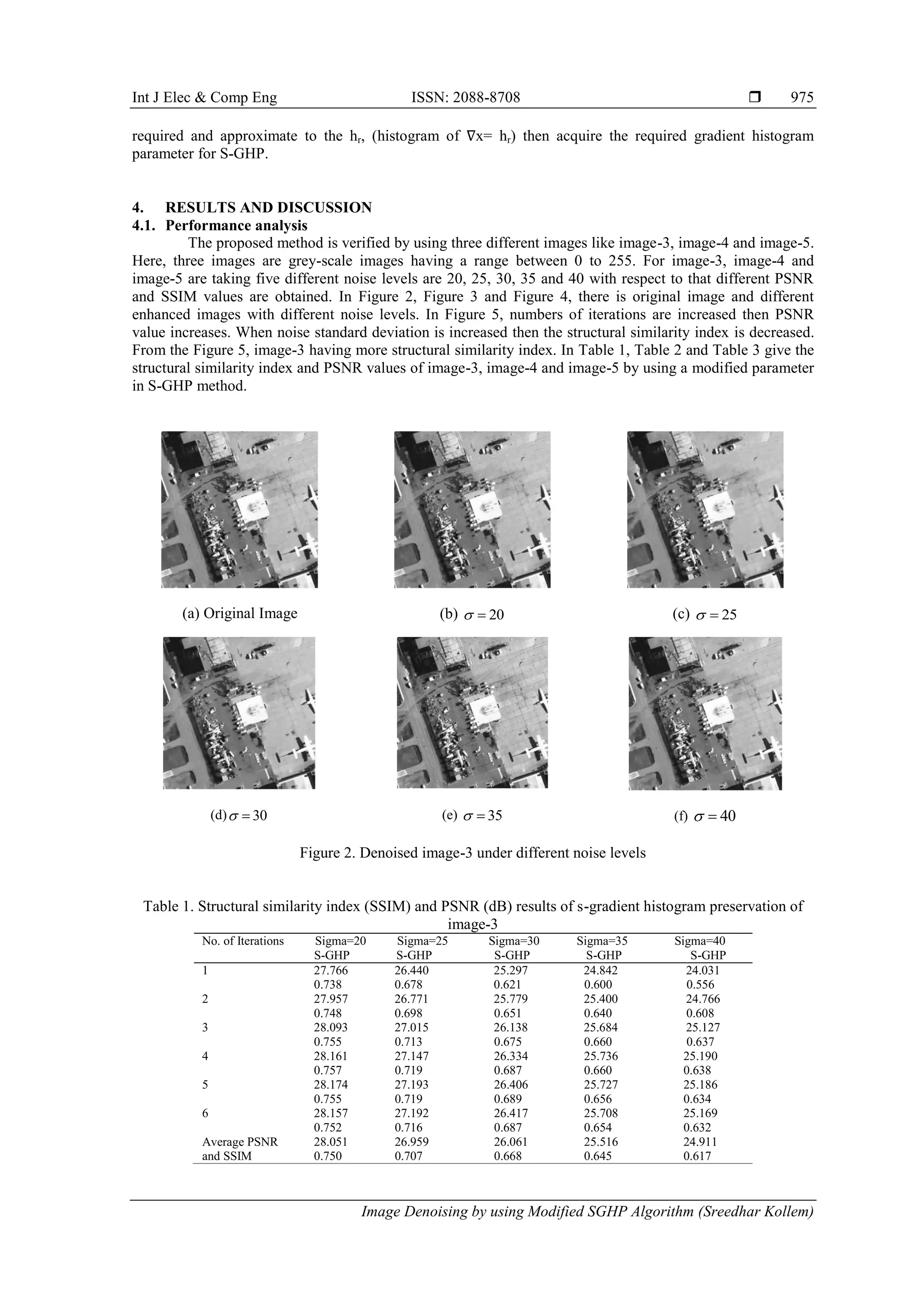
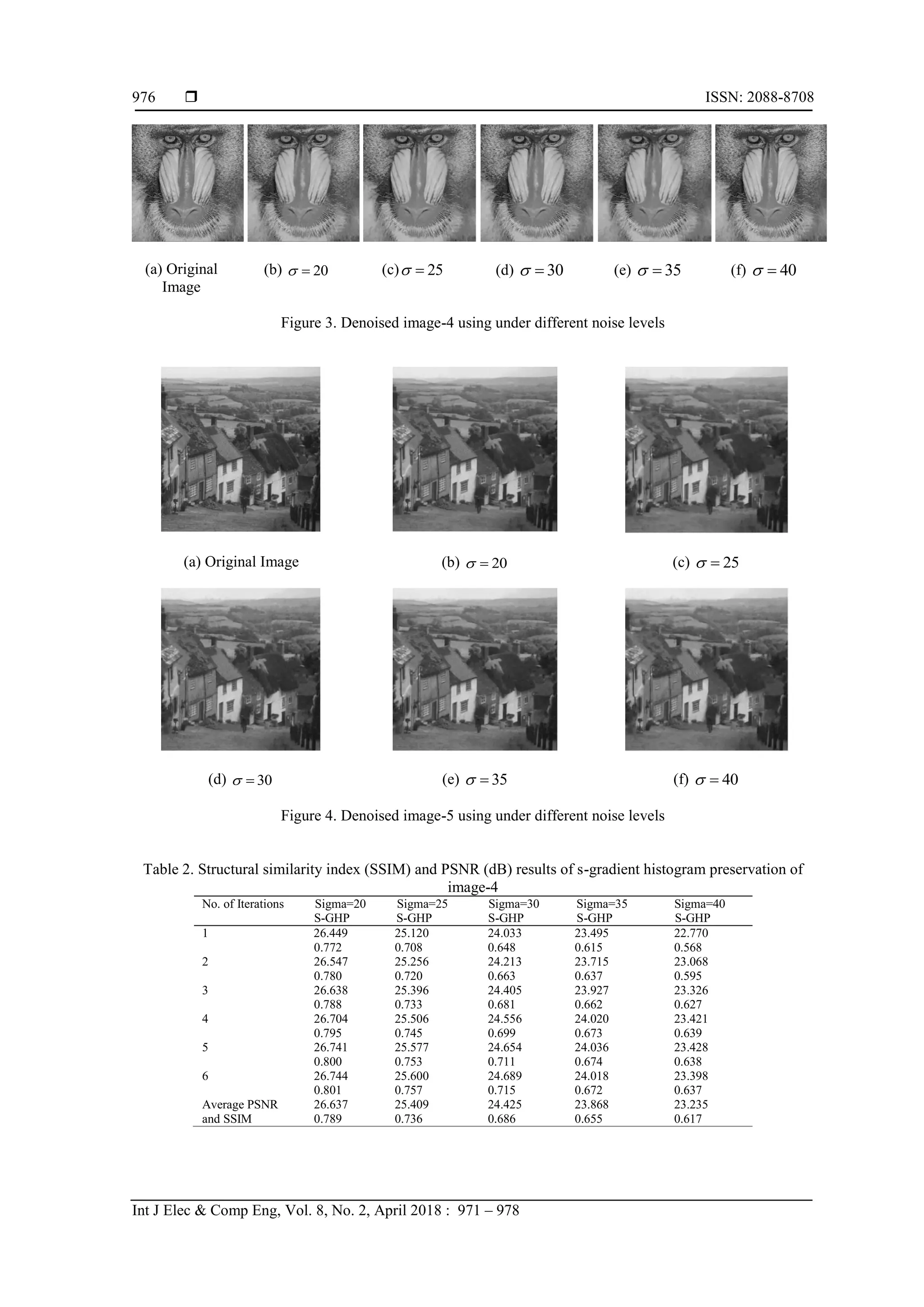
4.2. Comparative analysis
The existing methods and proposed method verified by using three different images like image-3,
image-4 and image-5 with five different noise levels are 20, 25, 30, 35 and 40. Performance of these methods
is mentioned in terms of Peak signal to noise ratio and structural similarity index [25], [26] as shown in
Table 4.
Table 4. Comparison of Existing methods and proposed method in terms of PSNR (dB) results
Image No Existing Methods Proposed Method
B-GHP APBS Modified S-GHP
PSNR PSNR
PSNR
3 27.01 26.05 28.051
4 25.49 25.11 26.637
5 29.90 28.66 30.288

 ISSN: 2088-8708
978
5. CONCLUSION
In this paper, the proposed method modified Structure gradient histogram preservation used for
enhancing the different images by taking different noise levels like 20, 25, 30 and 40. Based on the noise
levels, the PSNR and SSIM values are improved compared to other methods like APBS and B-GHP. All the
above-mentioned results proved that the modified parameter S-GHP is better compared to B-GHP and APBS.
REFERENCES
[1] Buades, B. Coll, and J. Morel, “A review of image denoising methods, with a new one”, Multiscale Model. Simul.,
vol. 4, no. 2, pp. 490530, 2005.
[2] K. Dabov, A. Foi, V. Katkovnik, and K. Egiazarian, “Image denoising by sparse 3-D transform-domain
collaborative filtering”, IEEE Trans. Image Process., vol. 16, no. 8, pp. 2080-2095, Aug. 2007.
[3] W. Dong, L. Zhang, G. Shi, and X. Li, “Nonlocally centralized sparse representation for image restoration”, IEEE
Trans. Image Process, vol. 22, no. 4, pp. 1620-1630, Apr. 2013.
[4] L. Rudin, S. Osher, and E. Fatemi, “Nonlinear total variation based noise removal algorithms”, Phys. D, vol. 60,
nos. 14, pp. 259-268, Nov. 1992.
[5] Pankaj Hedaoo and Swati S Godbole, “Wavelet Thresholding Approach for Image Denoising”, International
Journal of Network Security Its Applications (IJNSA), vol. 3, no. 4, July 2011.
[6] H. C. Burger, C. J. Schuler, and S. Harmeling, “Image denoising: Canplain neural networks compete with BM3D”,
in Proc. Int. Conf. CVPR, Jun. 2012, pp. 2392-2399.
[7] S. Subha, I. Jesudass and K. Thanushkodi, “Image denoising by using iterative histogram and preservative
algorithm”, ARPN Journal of Engineering and Applied Sciences, vol. 10, no. 11, June 2015.
[8] P. Koltsov, “Comparative study of texture detection and classification algorithms,” Comput. Math. Math. Phys.,
vol. 51, no. 8, pp. 1460-1466, 2011.
[9] Liu, Xinhao, Mitsuru Tanaka, and Masatoshi Okutomi, “Noise level estimation using weak textured patches of a
single noisy image”, Image Processing (ICIP), 2012 19th IEEE International Conference on. IEEE, 2012.
[10] S. Pyatykh, J. Hesser and L. Zheng, "Image Noise Level Estimation by Principal Component Analysis," in IEEE
Transactions on Image Processing, vol. 22, no. 2, pp. 687-699, Feb. 2013.doi: 10.1109/TIP.2012.2221728.
[11] Jolliffe, “Principal component analysis,” in Encyclopedia of Statistics in Behavioral Science. New York: Springer-
Verlag, 2002.
[12] D. Pastor, “A theoretical result for processing signals that have unknown distributions and priors in white Gaussian
noise,” Comput. Stat. Data Anal., vol. 52, no. 6, pp. 3167–3186, 2008.
[13] Liu, “A fast method of estimating Gaussian noise,” in Proc. 1st Int. Conf. Inf. Sci. Eng., 2009, pp. 441–444.
[14] C. Kervrann and J. Boulanger, “Optimal spatial adaptation for patch-based image denoising,” IEEE Trans. Image
Process., vol. 15, no. 10, pp. 2866–2878, Oct. 2006.
[15] R. Bilcu and M. Vehvilainen, “New method for noise estimation in images,” in Proc. IEEE-Eurasip Nonlinear
Signal Image Process., May 2005.
[16] G. Smith and I. Burns, “Measuring texture classification algorithms,” Pattern Recognit. Lett., vol. 18, no. 14, pp.
1495–1501, 1997.
[17] D. Makovoz, “Noise variance estimation in signal processing,” in Proc. IEEE Int. Symp. Signal Process. Inf.
Technol., Jul. 2006, pp. 364–369.
[18] M. Uss, B. Vozel, V. Lukin, S. Abramov, I. Baryshev, and K. Chehdi, “Image informative maps for estimating noise
standard deviation and texture parameters,” EURASIP J. Adv. Signal Process., vol. 2011, pp. 806516-1–806516-12,
Mar. 2011.
[19] M. Elad and M. Aharon, “Image denoising via sparse and redundant representations over learned dictionaries”,
IEEE Trans. Image Process., vol. 15, no. 12, pp. 3736-3745, Dec. 2006.
[20] J. Jancsary, S. Nowozin, and C. Rother, “Loss-specific training of nonparametric image restoration models: a new
state of the art,” in Proc. Eur. Conf. Comput. Vis., 2012.
[21] M. Hashemi and S. Beheshti, “Adaptive noise variance estimation in Bayes shrink”, IEEE Signal Process. Lett.,
vol. 17, no. 1, pp. 12-15, Jan. 2010.
[22] T. Tasdizen, “Principal components for non-local means image denoising,” in Proc. IEEE Int. Conf. Image Process.,
Feb. 2008, pp. 1728-1731.
[23] V. Rajanesh and Kollem Sreedhar, “A New Approach to Image Denoising by Patch-Based Algorithm”, in
International Journal of Advanced Research in Computer and Communication Engineering, vol. 5, no. 12,
pp. 212-218, 2016.
[24] Yasmin, Sabina, and Md Masud Rana, “Performance Study of Soft Local Binary Pattern over Local Binary Pattern
under Noisy Images”, International Journal of Electrical and Computer Engineering, vol. 6, no. 3 (2016), p. 1161.
[25] Omidiora, E. O., S. O. Olabiyisi, J. A. Ojo, Abayomi-Alli Adebayo, O. Abayomi-Alli, and K. B. Erameh, “Facial
Image Verification and Quality Assessment System-FaceIVQA”, International Journal of Electrical and Computer
Engineering, vol. 3, no. 6 (2013), p. 863.
[26] Subramanyam, M. V., and Giri Prasad, “A New Approach for SAR Image Denoising”, International Journal of
Electrical and Computer Engineering, vol. 5, no. 5 (2015).

Image Denoising by using Modified SGHP Algorithm

More Related Content

What's hot

Similar to Image Denoising by using Modified SGHP Algorithm

More from IJECEIAES

Recently uploaded

Image Denoising by using Modified SGHP Algorithm