Deep Learning Sample Class (Jon Lederman)

Deep Learning and
TensorFlow
Sample Class
Jon Lederman

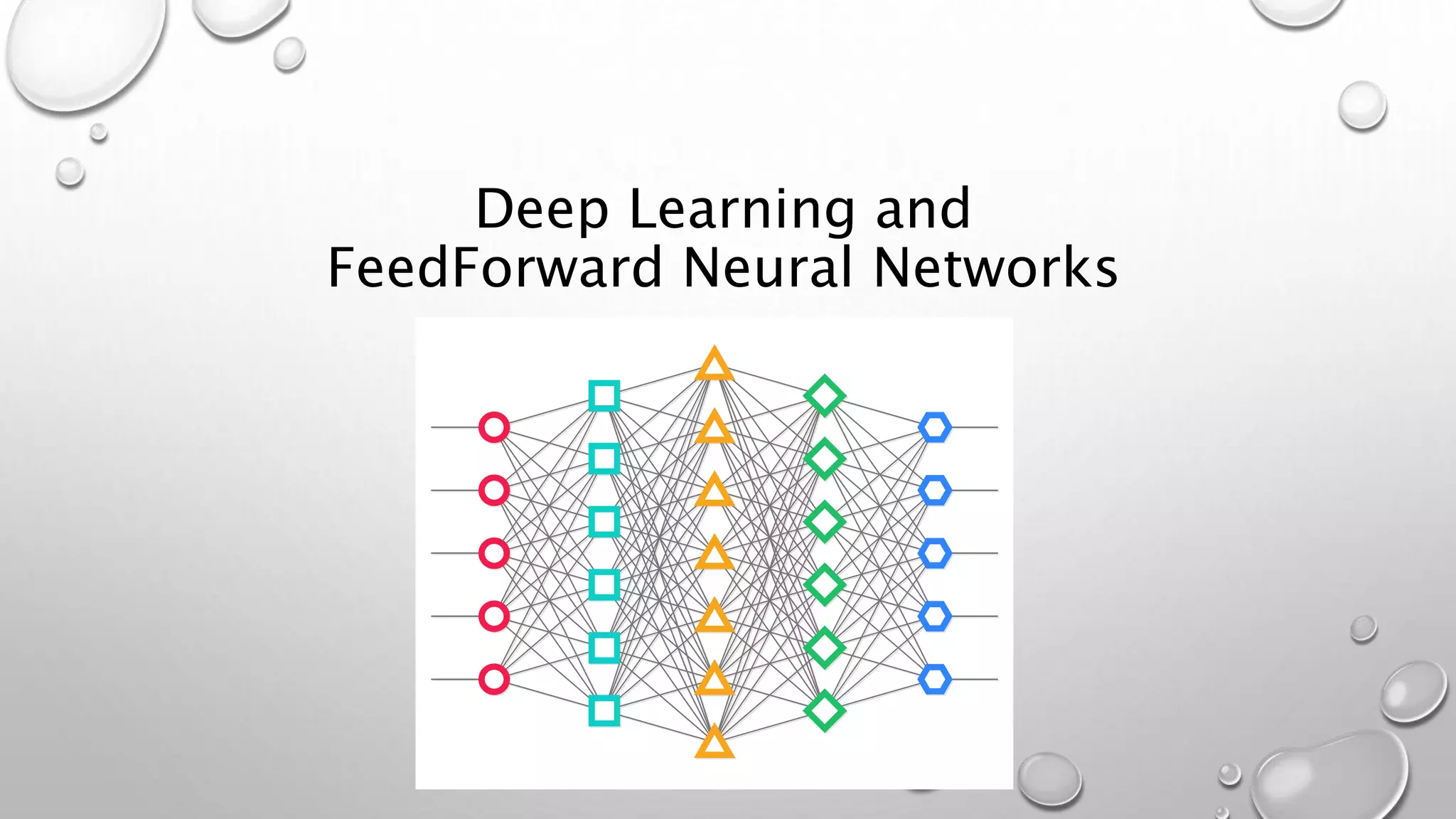
Deep Learning and
FeedForward Neural Networks

Features/Representations
• Features or representations:
• Measurable property or characteristic of a phenomenon being observed
• Specific variables that are provided as input to an algorithm
• The success of a machine learning algorithm depends on determining the right
features
• With the right features, a machine learning algorithm can learn almost anything
• With the wrong features, performance will be abysmal
• But how do we decide what are the good features?

Examples of Features
• Character Recognition
• Histograms counting number of black pixels along horizontal and vertical directions,
number of internal holes, stroke detection, etc.
• Speech Recognition
• Mel frequency cepstral coefficients, phonemes, noise ratios, length of sound, etc.
• Computer Vision
• Edges, objects, colors, etc.

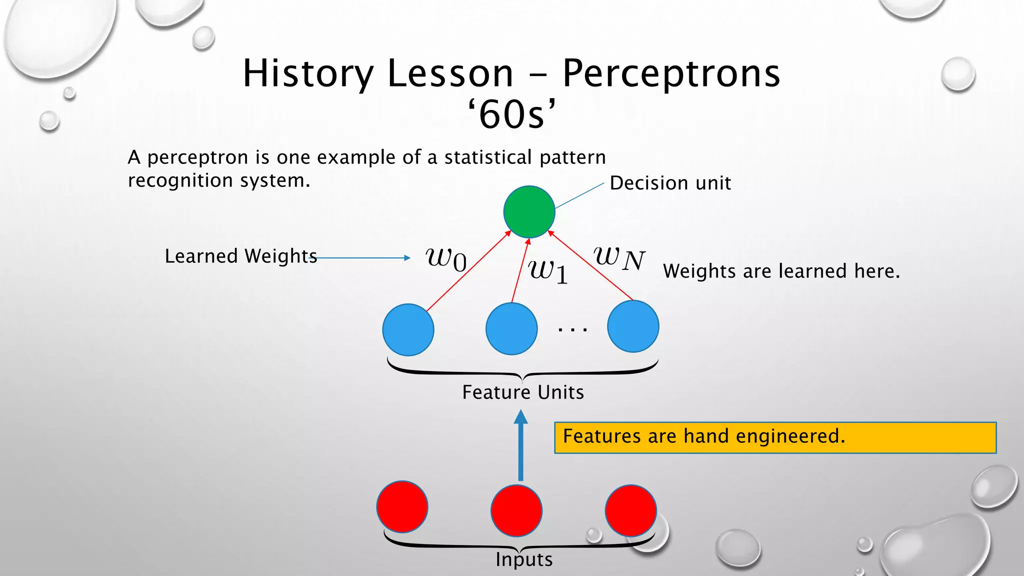
History Lesson - Perceptrons
‘60s’
A perceptron is one example of a statistical pattern
recognition system.
. . .
Decision unit
Learned Weights
Feature Units
Inputs
Features are hand engineered.
Weights are learned here.

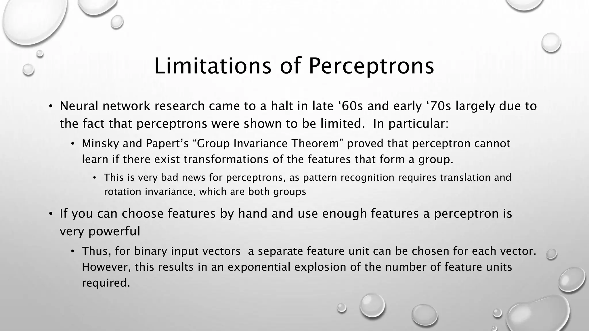
Limitations of Perceptrons
• Neural network research came to a halt in late ‘60s and early ‘70s largely due to
the fact that perceptrons were shown to be limited. In particular:
• Minsky and Papert’s “Group Invariance Theorem” proved that perceptron cannot
learn if there exist transformations of the features that form a group.
• This is very bad news for perceptrons, as pattern recognition requires translation and
rotation invariance, which are both groups
• If you can choose features by hand and use enough features a perceptron is
very powerful
• Thus, for binary input vectors a separate feature unit can be chosen for each vector.
However, this results in an exponential explosion of the number of feature units
required.

Hallmarks of Deep Learning
(Lessons From Perceptrons)
• Feature Learning or Representational Learning
• Deep neural networks learn their own feature detectors (more on this later)
• Hierarchical Learning
• More complex representations are expressed in terms of simpler representations
• Non-linear
• Deep Neural Networks have non-linearity “baked” into the neuron model. This
allows them to learn much more complex features
• Most of the interesting complexities of the world are non-linear
• Superposition does not apply
• Linear networks can only learn linear things as composition of linear operator is still linear

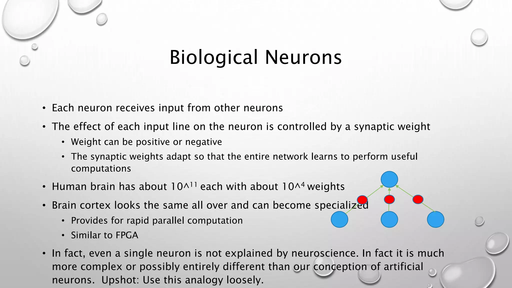
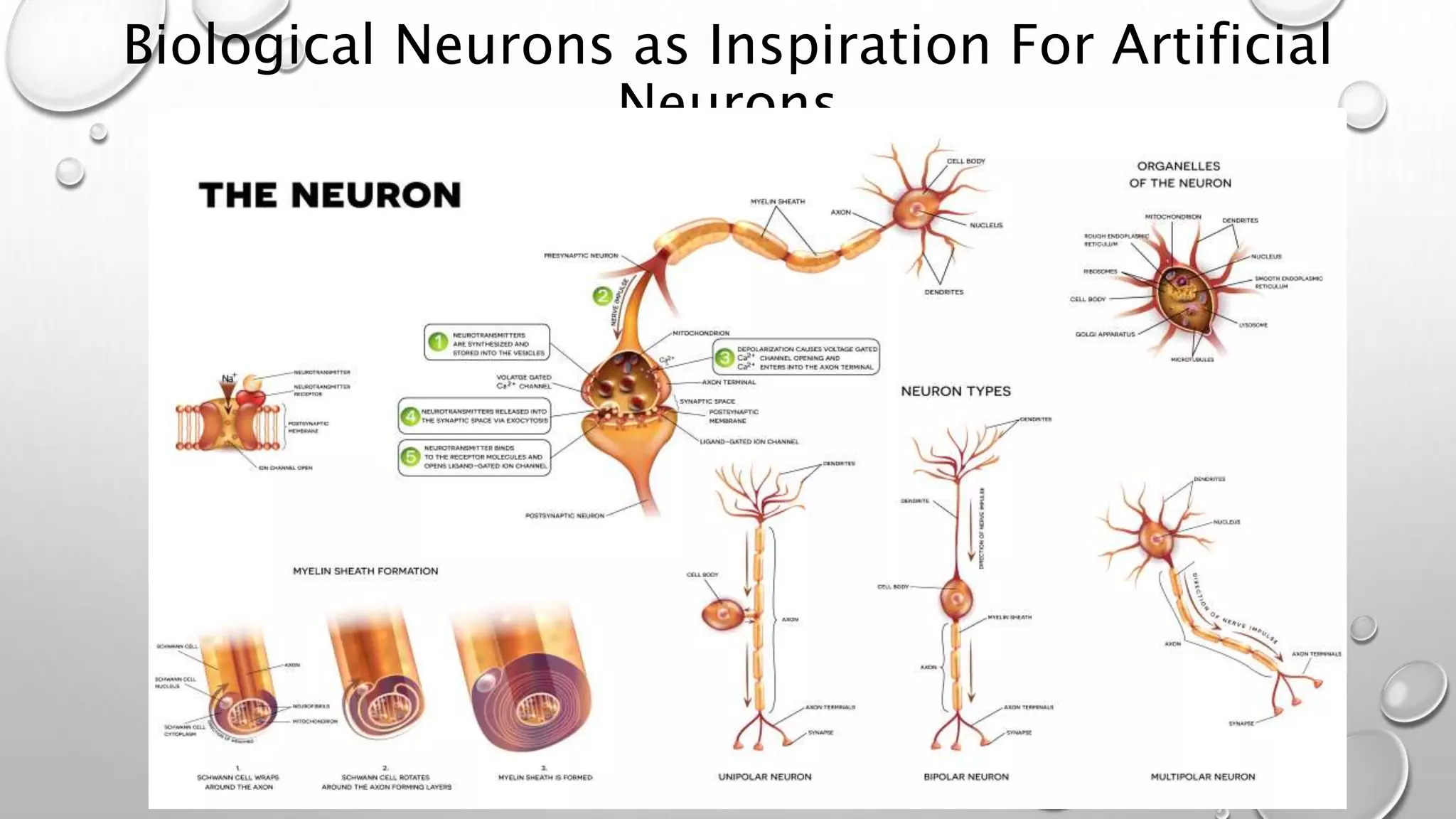
Biological Neurons
• Each neuron receives input from other neurons
• The effect of each input line on the neuron is controlled by a synaptic weight
• Weight can be positive or negative
• The synaptic weights adapt so that the entire network learns to perform useful
computations
• Human brain has about 10^11 each with about 10^4 weights
• Brain cortex looks the same all over and can become specialized
• Provides for rapid parallel computation
• Similar to FPGA
• In fact, even a single neuron is not explained by neuroscience. In fact it is much
more complex or possibly entirely different than our conception of artificial
neurons. Upshot: Use this analogy loosely.

Biological Neurons as Inspiration For Artificial
Neurons

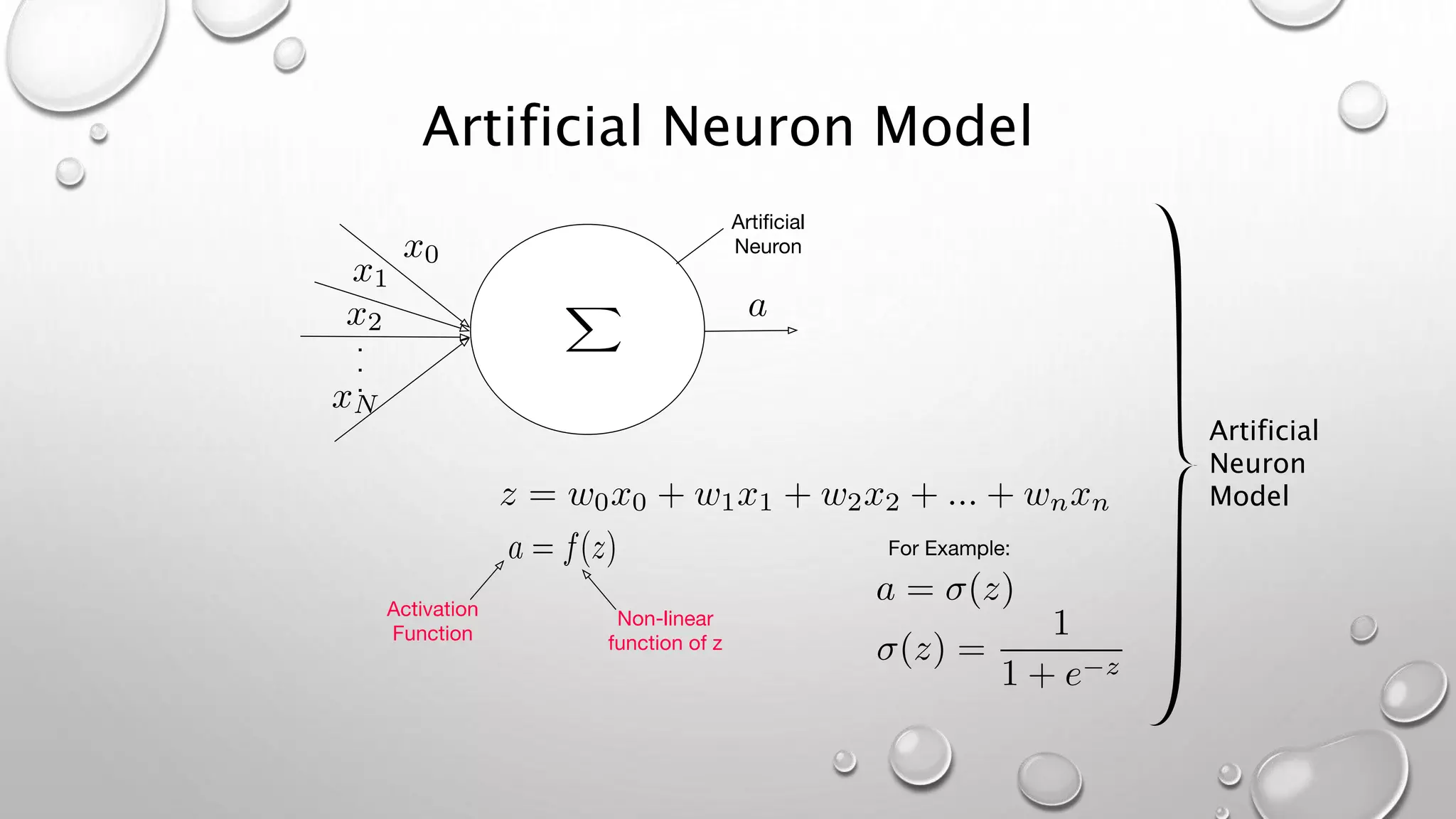
Artificial Neuron Model
Artificial
Neuron
Model

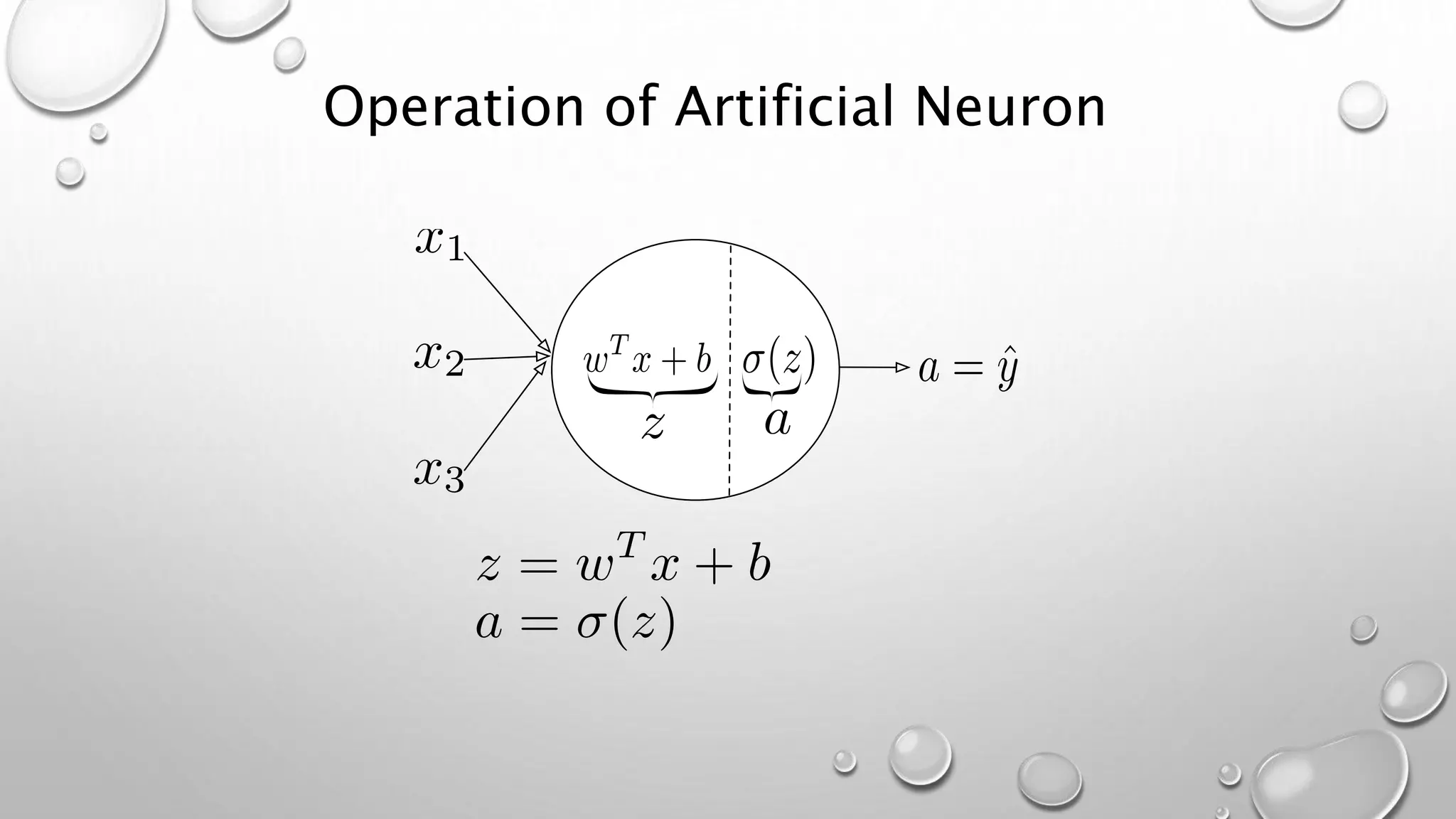
Operation of Artificial Neuron

But What is “Learning” and How Does It
Happen?
• Deep learning is a form of supervised learning
• We build a network of artificial neurons which takes in an input and generates some
output
• Input can be a single number or can be a vector
• We show the network a series of training examples and ask the network to learn
from these examples
• The training examples consist of an input and a (hopefully) correct output called the
“ground truth”
Deep Feedforward Networks
Multilayer Neural Networks
.
.
.
.
.
.
Input Hidden Unit Output
.
.
.
.
.
.
.
.
.
.
.
.
.
.
.
.
.
.
Input Layer Output LayerHidden Layers
a[0]
= x a[1] a[2]
a[l]
ˆy = a[L ]
Combine a bunch of
artificial neurons into
layers and let them
talk to one another!

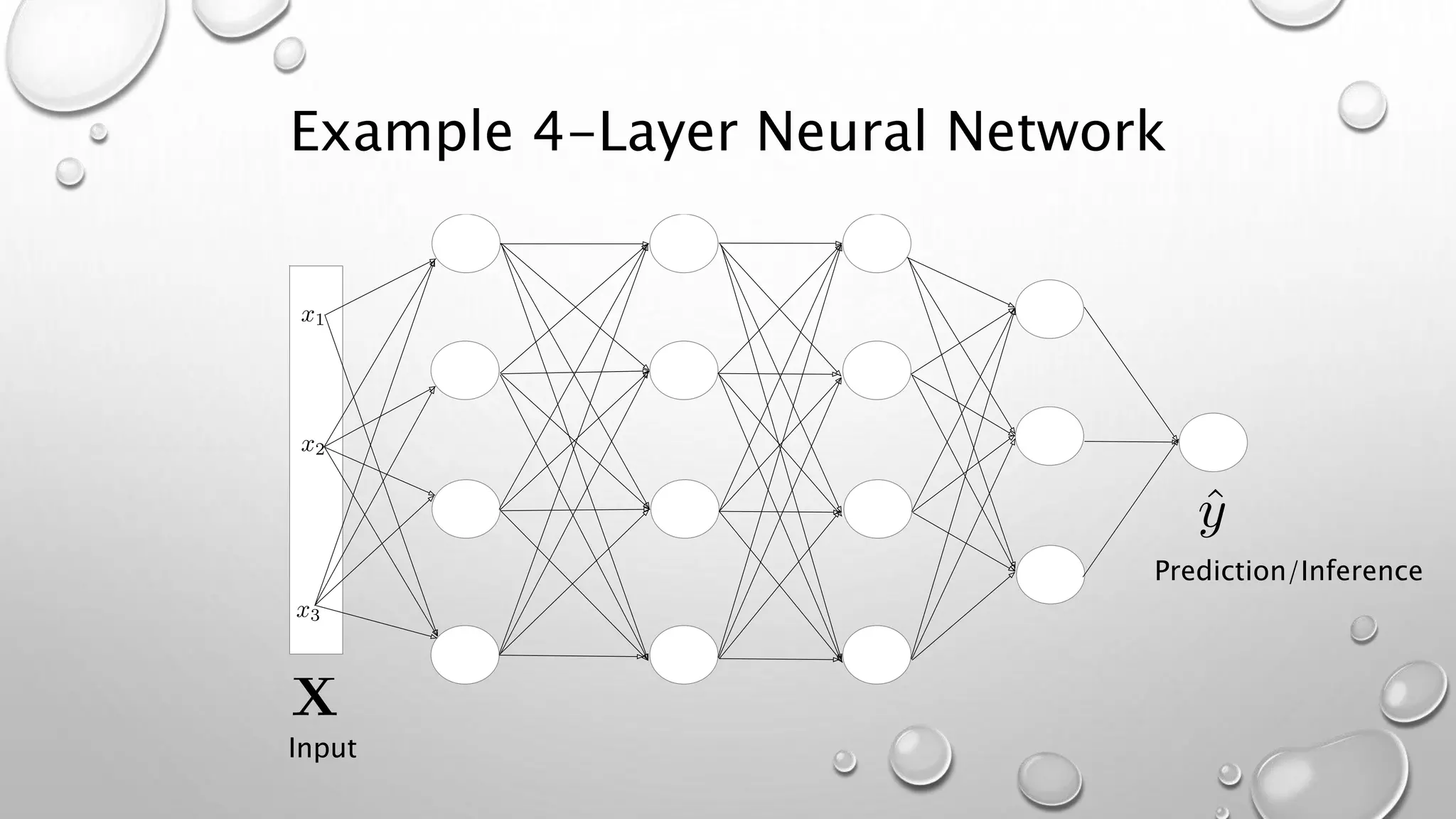
Example 4-Layer Neural Network
Input
Prediction/Inference

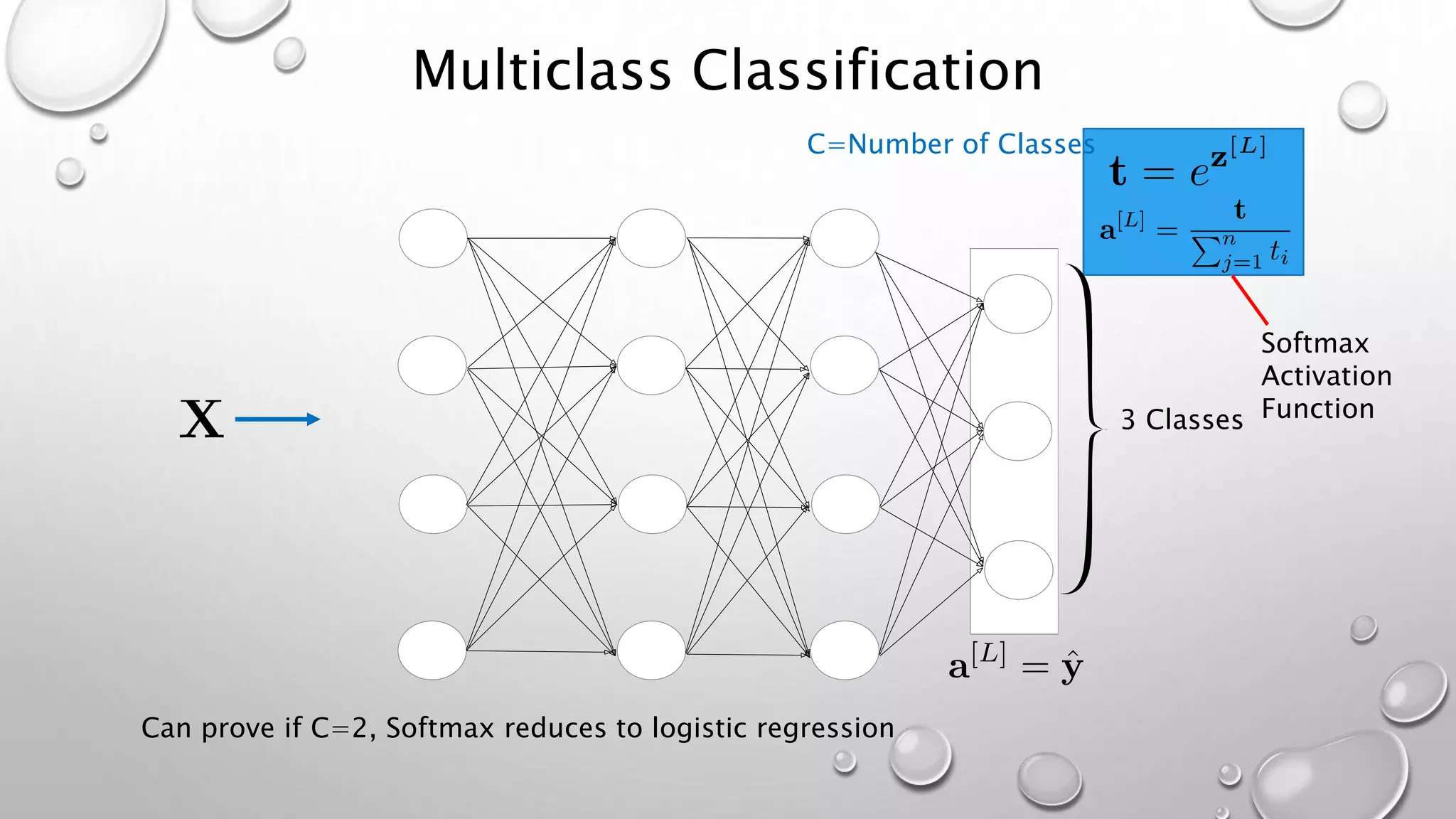
Multiclass Classification
3 Classes
C=Number of Classes
Softmax
Activation
Function
Can prove if C=2, Softmax reduces to logistic regression

Two Questions About Neural Networks
• What does a neural network do?
• How does a neural network learn?
• What is the learning mechanism?

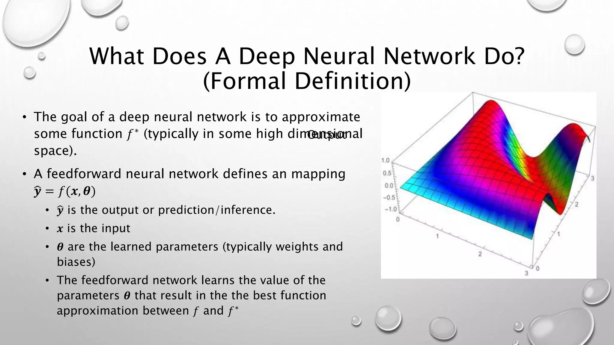
What Does A Deep Neural Network Do?
(Formal Definition)
• The goal of a deep neural network is to approximate
some function 𝑓∗
(typically in some high dimensional
space).
• A feedforward neural network defines an mapping
𝒚 = 𝑓(𝒙, 𝜽)
• 𝒚 is the output or prediction/inference.
• 𝒙 is the input
• 𝜽 are the learned parameters (typically weights and
biases)
• The feedforward network learns the value of the
parameters 𝜽 that result in the the best function
approximation between 𝑓 and 𝑓∗
Output

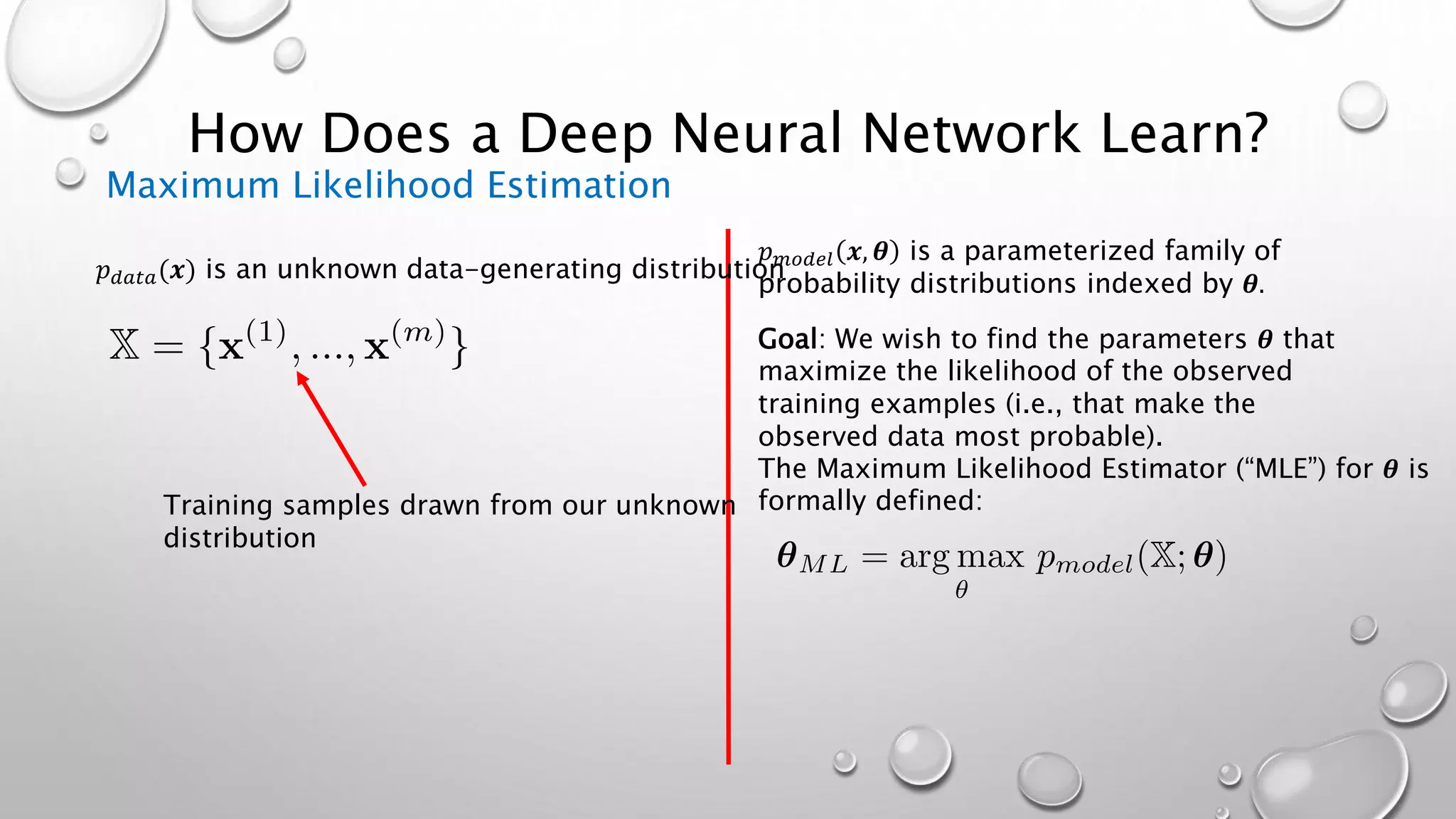
How Does a Deep Neural Network Learn?
Maximum Likelihood Estimation
𝑝 𝑑𝑎𝑡𝑎(𝒙) is an unknown data-generating distribution
Training samples drawn from our unknown
distribution
𝑝 𝑚𝑜𝑑𝑒𝑙 𝒙, 𝜽 is a parameterized family of
probability distributions indexed by 𝜽.
Goal: We wish to find the parameters 𝜽 that
maximize the likelihood of the observed
training examples (i.e., that make the
observed data most probable).
The Maximum Likelihood Estimator (“MLE”) for 𝜽 is
formally defined:

How Does a Deep Neural Network Learn?
Maximum Likelihood Estimation
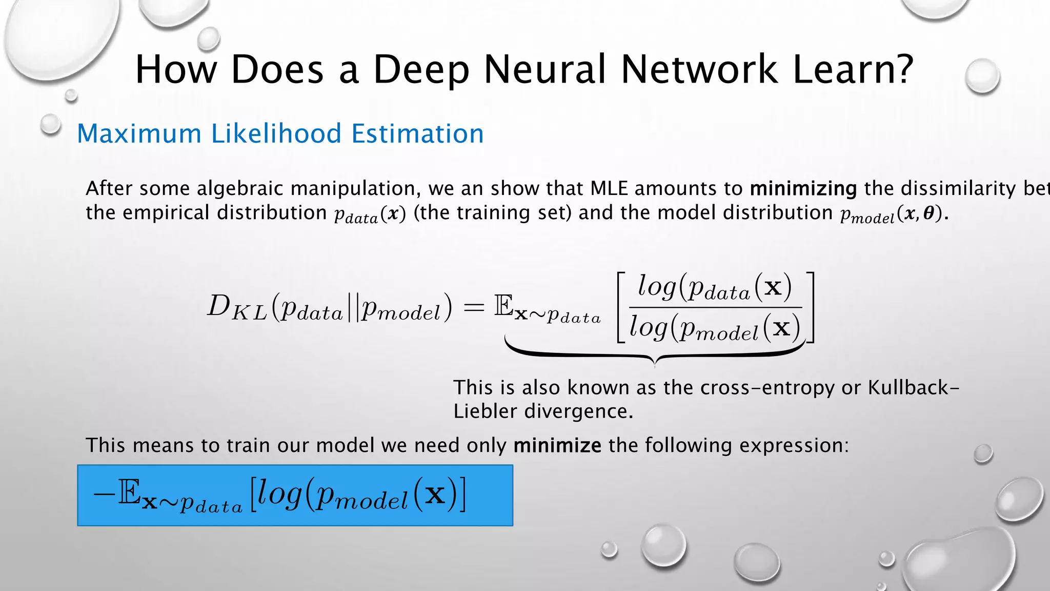
After some algebraic manipulation, we an show that MLE amounts to minimizing the dissimilarity bet
the empirical distribution 𝑝 𝑑𝑎𝑡𝑎(𝒙) (the training set) and the model distribution 𝑝 𝑚𝑜𝑑𝑒𝑙 𝒙, 𝜽 .
This is also known as the cross-entropy or Kullback-
Liebler divergence.
This means to train our model we need only minimize the following expression:

Supervised Learning
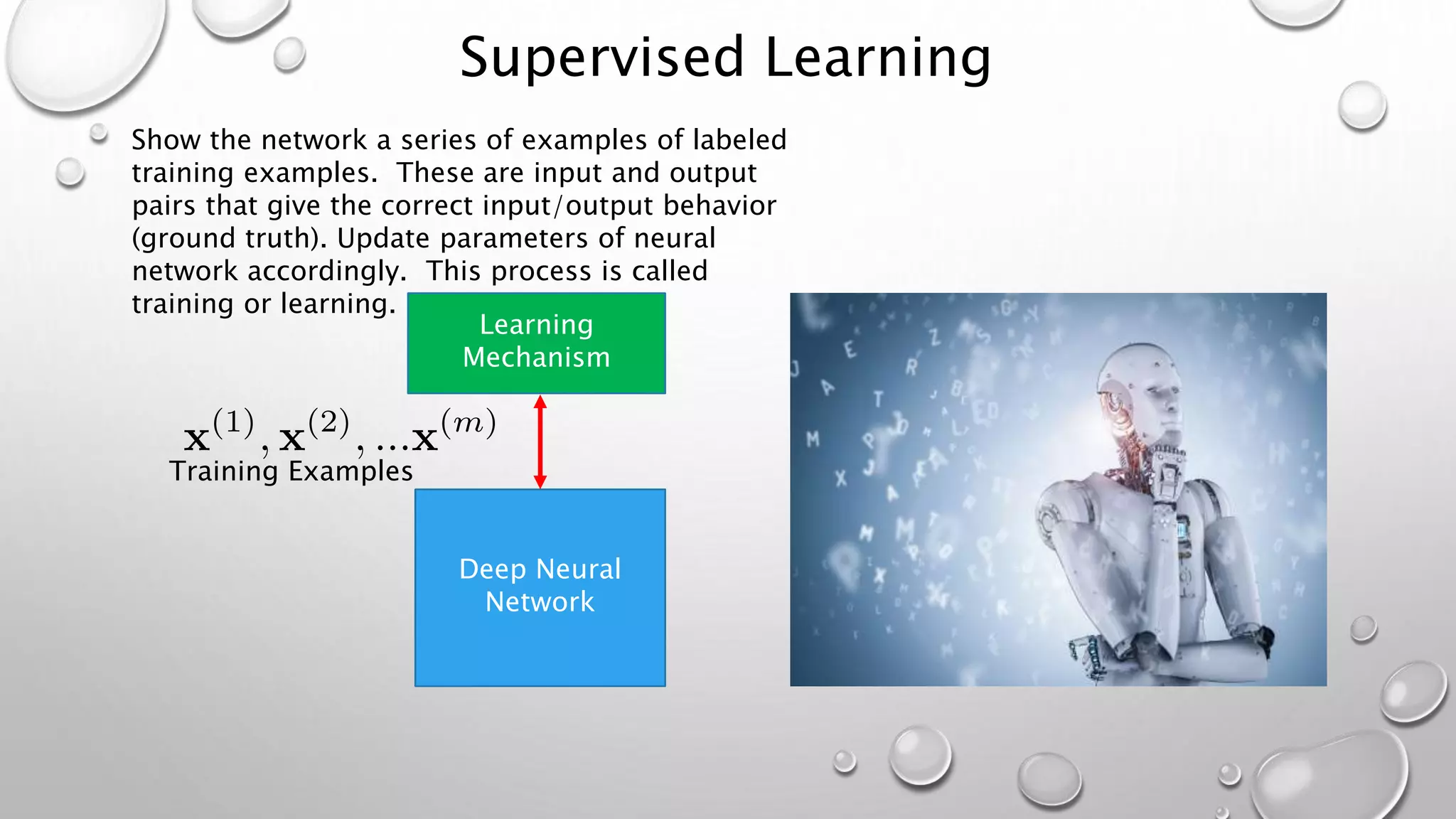
Show the network a series of examples of labeled
training examples. These are input and output
pairs that give the correct input/output behavior
(ground truth). Update parameters of neural
network accordingly. This process is called
training or learning.
Deep Neural
Network
Learning
Mechanism
Training Examples

Learning Mechanism
(High Level)
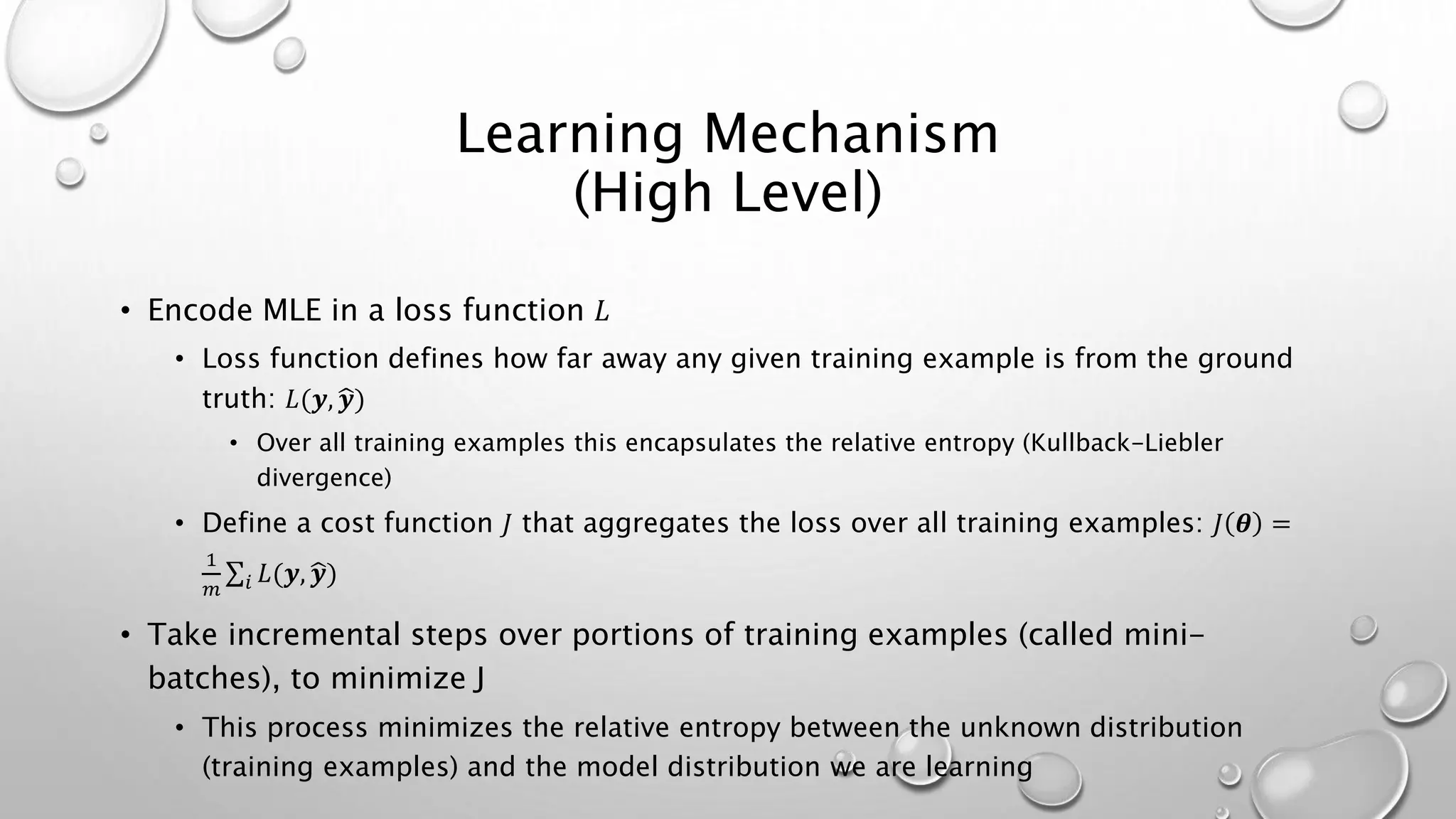
• Encode MLE in a loss function 𝐿
• Loss function defines how far away any given training example is from the ground
truth: 𝐿(𝒚, 𝒚)
• Over all training examples this encapsulates the relative entropy (Kullback-Liebler
divergence)
• Define a cost function 𝐽 that aggregates the loss over all training examples: 𝐽 𝜽 =
1
𝑚 𝑖 𝐿(𝒚, 𝒚)
• Take incremental steps over portions of training examples (called mini-
batches), to minimize J
• This process minimizes the relative entropy between the unknown distribution
(training examples) and the model distribution we are learning

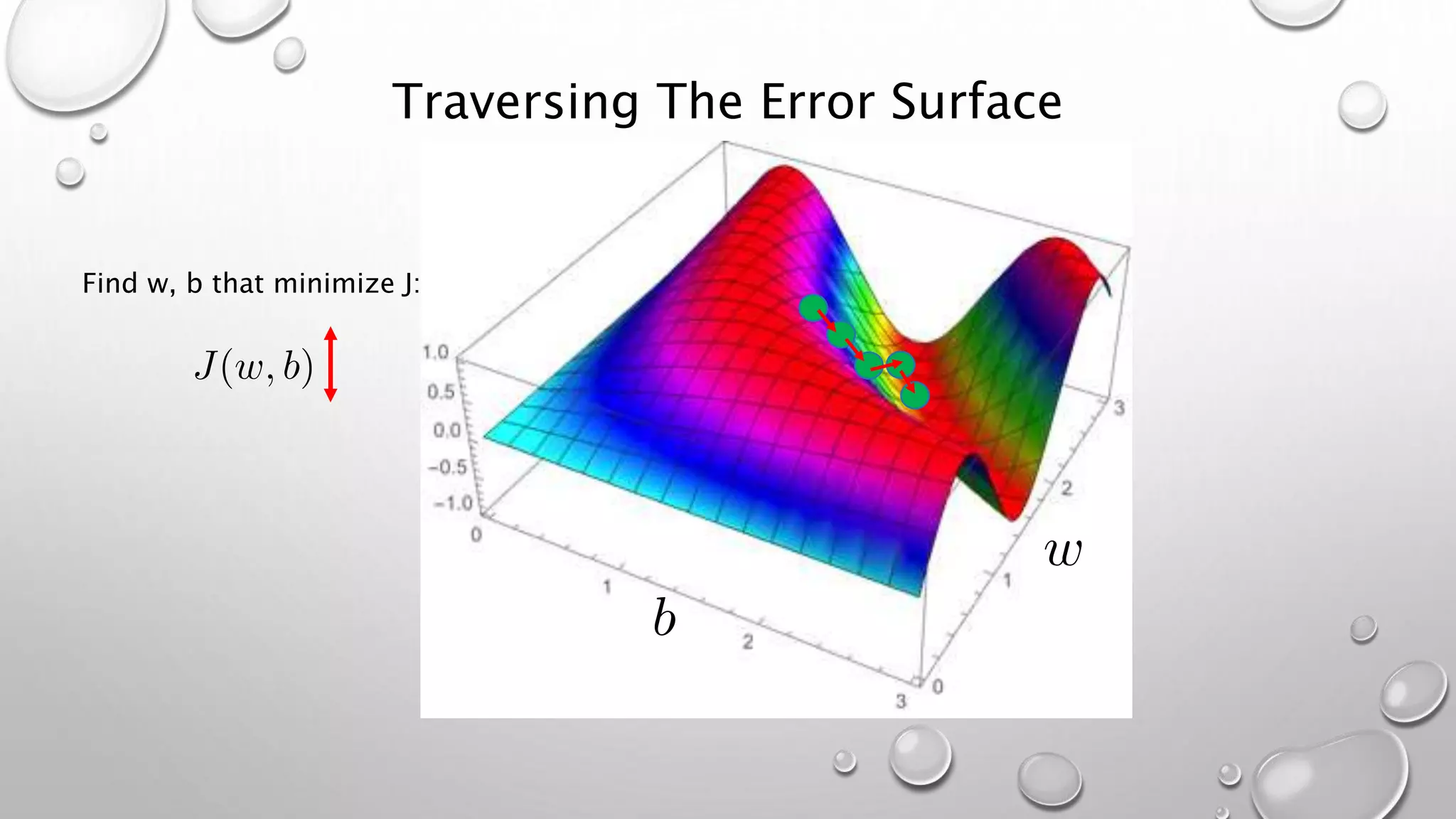
Traversing The Error Surface
Find w, b that minimize J:

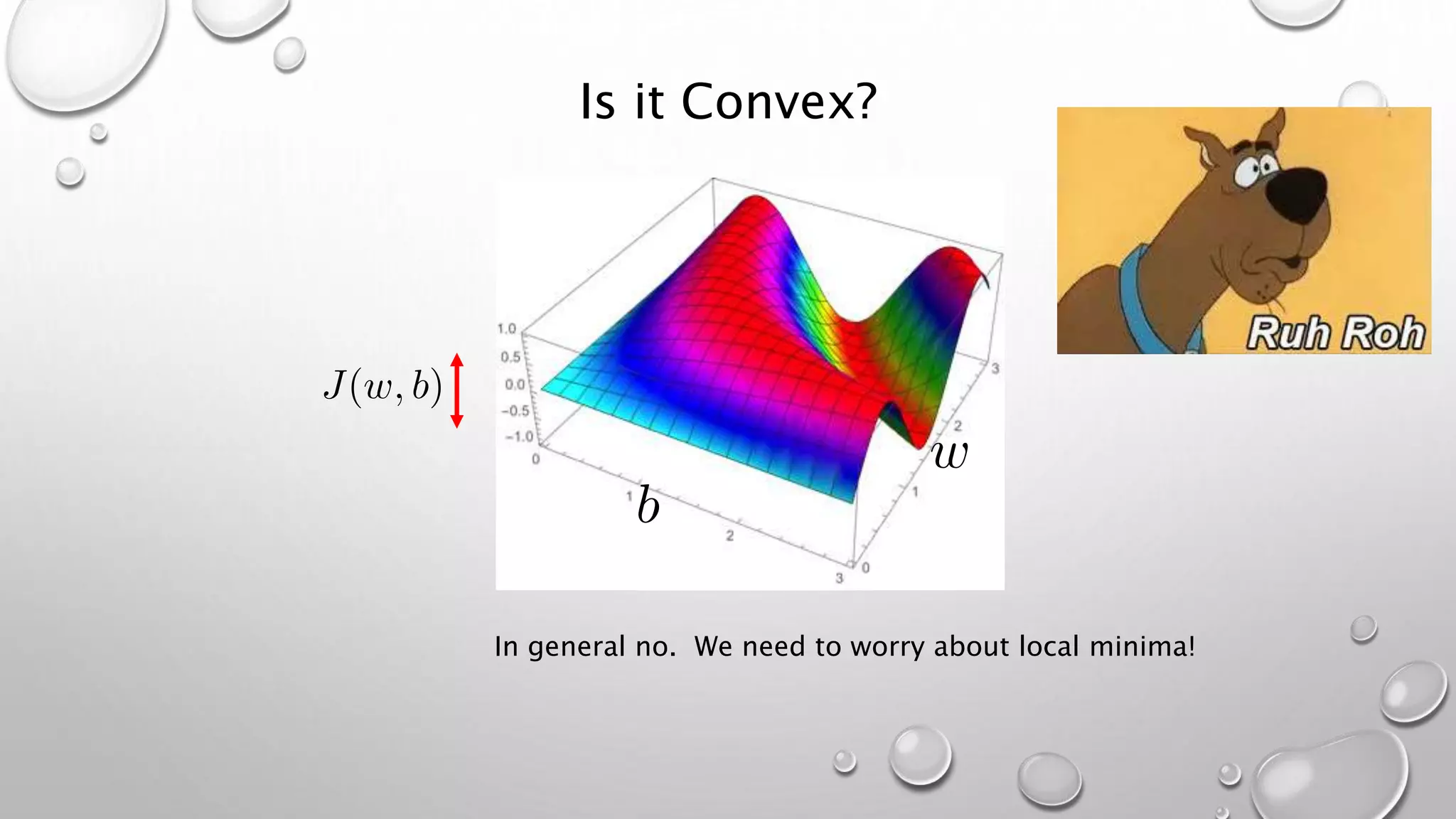
Is it Convex?
In general no. We need to worry about local minima!

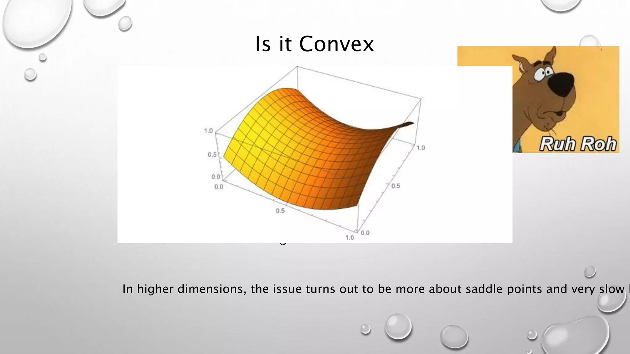
Is it Convex
In higher dimensions, the issue turns out to be more about saddle points and very slow l

How Do Deep Neural Networks Learn Their
Own Feature Detectors?
• The learned parameters (weights and biases) are the feature detectors
• We let the network decide what features are important as expressed through the
weights and biases
• Each hidden layer/hidden unit may learn a different feature

Mechanics of Learning
• ForwardPropagation
• Update a’s and z’s based on next training example
• Cache this information for backpropagation
• BackPropagation
• Compute Gradients dW, db
• Gradient Descent
• Take small step on error surface in direction of gradients

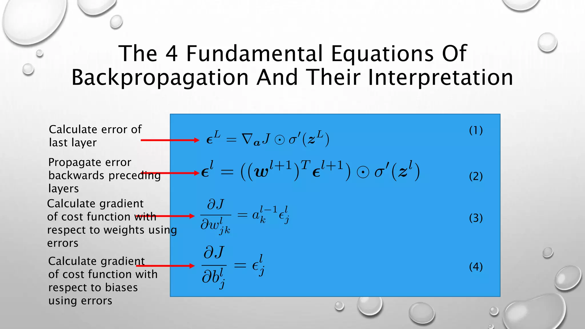
The 4 Fundamental Equations Of
Backpropagation And Their Interpretation
(1)
(2)
(3)
(4)
Calculate error of
last layer
Propagate error
backwards preceding
layers
Calculate gradient
of cost function with
respect to weights using
errors
Calculate gradient
of cost function with
respect to biases
using errors

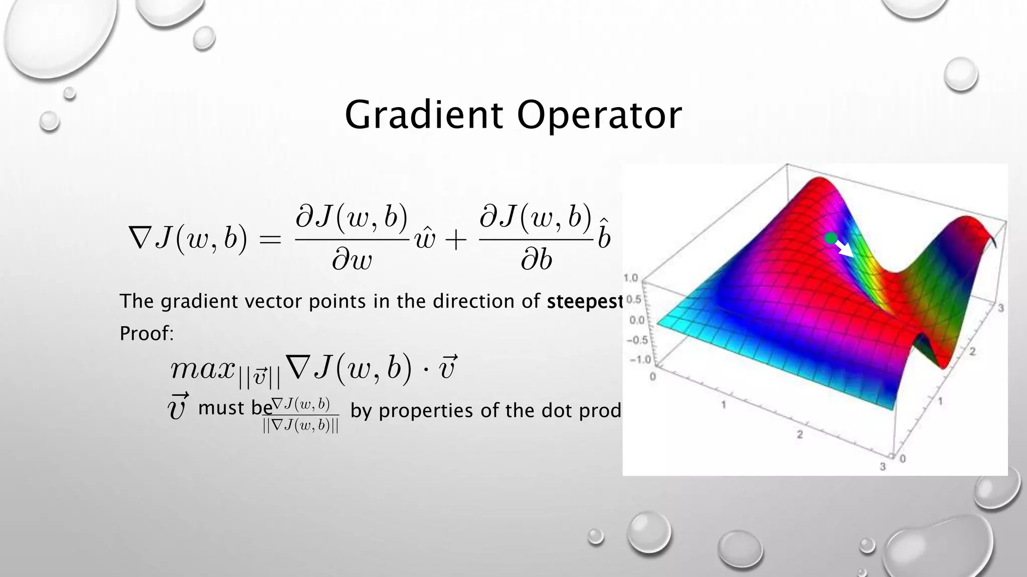
Gradient Operator
The gradient vector points in the direction of steepest ascent.
Proof:
must be by properties of the dot product.

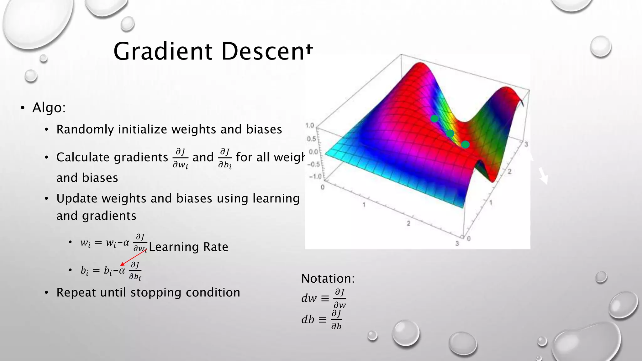
Gradient Descent
• Algo:
• Randomly initialize weights and biases
• Calculate gradients
𝜕𝐽
𝜕𝑤 𝑖
and
𝜕𝐽
𝜕𝑏 𝑖
for all weights
and biases
• Update weights and biases using learning rate
and gradients
• 𝑤𝑖 = 𝑤𝑖-𝛼
𝜕𝐽
𝜕𝑤 𝑖
• 𝑏𝑖 = 𝑏𝑖-𝛼
𝜕𝐽
𝜕𝑏 𝑖
• Repeat until stopping condition
Notation:
𝑑𝑤 ≡
𝜕𝐽
𝜕𝑤
𝑑𝑏 ≡
𝜕𝐽
𝜕𝑏
Learning Rate

Backpropagation With Gradient Descent
• For each training example x, set the input activation 𝒂[0](𝑥) and perform the
following steps:
• Feedforward: For each l=1, 2, 3, … L compute 𝒛[𝑙](𝑥) = 𝒘[𝑙] 𝒂 𝑙−1 (𝑥) + 𝒃[𝑙] and 𝒂[𝑙](𝑥) =
𝜎(𝒛 𝑙
)
• Output Error: Compute 𝜺[𝐿](𝑥) = 𝜵 𝒂 𝐽⨀𝜎′(𝒛[𝐿](𝑥))
• Backpropagate Error: For each i=L-l, L-2 , … 1 compute 𝜺[𝑙](𝑥) =
((𝒘[𝑙+1]) 𝑇 𝜺[𝑙+1](𝑥))⨀𝜎′(𝒛[𝑙](𝑥))
• Compute One Step Of Gradient Descent: For each l=L, L-1, L-2, … 1, update the
weights according to the rules:
• 𝒘𝑙
= 𝒘𝑙
−
∝
𝑚 𝑥 𝜺 𝑙 𝑥
(𝒂 𝑙−1 𝑥
) 𝑇
• 𝒃𝑙
= 𝒃𝑙
−
𝛼
𝑚 𝑥 𝜺 𝑙 𝑥
Learning Rate
Learning Rate

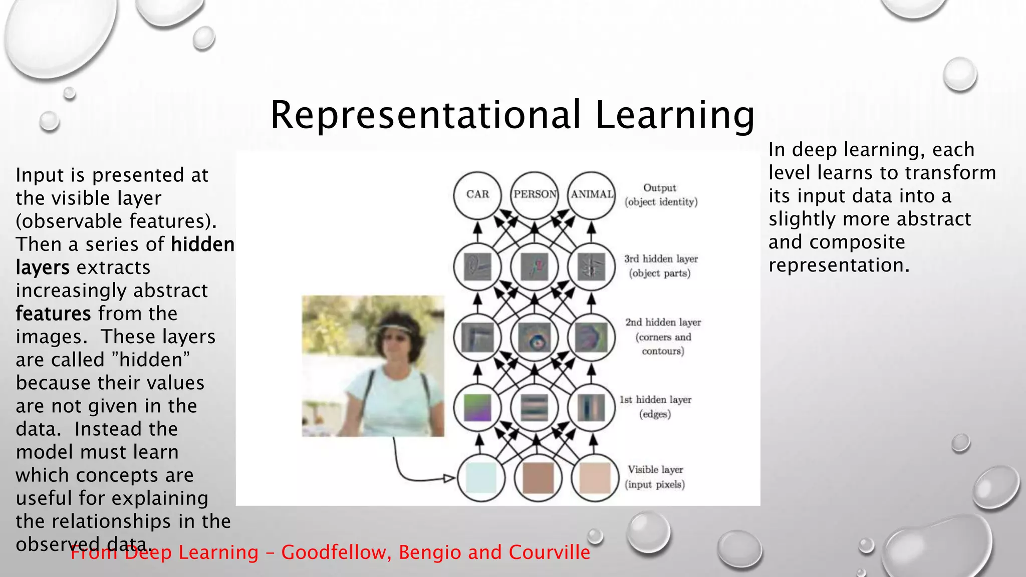
Representational Learning
From Deep Learning – Goodfellow, Bengio and Courville
Input is presented at
the visible layer
(observable features).
Then a series of hidden
layers extracts
increasingly abstract
features from the
images. These layers
are called ”hidden”
because their values
are not given in the
data. Instead the
model must learn
which concepts are
useful for explaining
the relationships in the
observed data.
In deep learning, each
level learns to transform
its input data into a
slightly more abstract
and composite
representation.

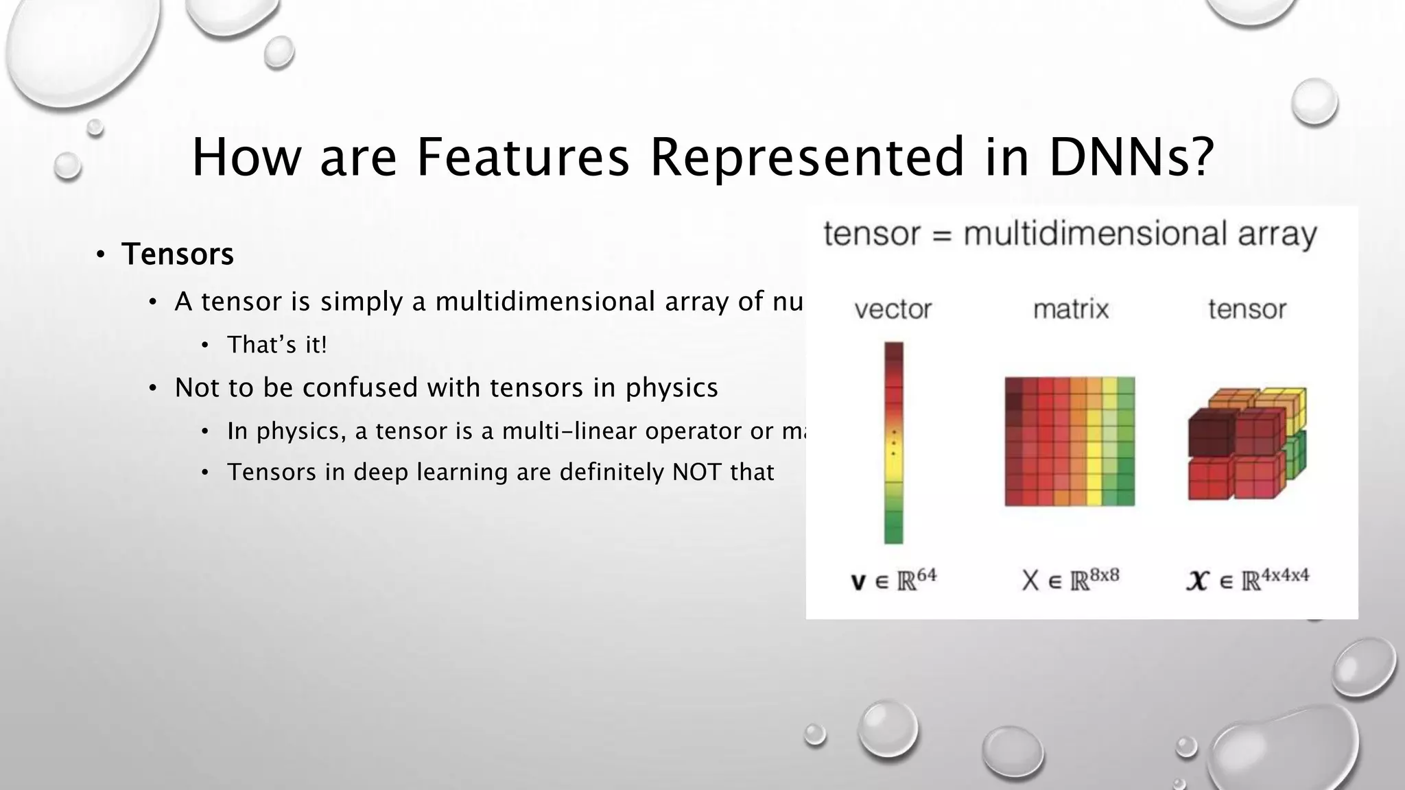
How are Features Represented in DNNs?
• Tensors
• A tensor is simply a multidimensional array of numbers
• That’s it!
• Not to be confused with tensors in physics
• In physics, a tensor is a multi-linear operator or map
• Tensors in deep learning are definitely NOT that

Deep Neural Networks as Feature Detectors
• AlexNet (Sneak preview)
• Convolutional neural network that achieved a top-5 error of 15.3%, more than 10.8
percentage points ahead of the runner up in ImageNet Large Scale Visualization
Recognition Challenge
• Think of convolutional network as:
• Feature detectors – Conv layers that detect features
• Fully connected feedforward layers – compose features detected by conv layers into more complex
representations
• Will discuss convolutional neural networks in depth later
• AlexNet has 8 layers
• 5 Convolutional Layers – Feature Detectors
• 3 Fully Connected Layers – Compose Features

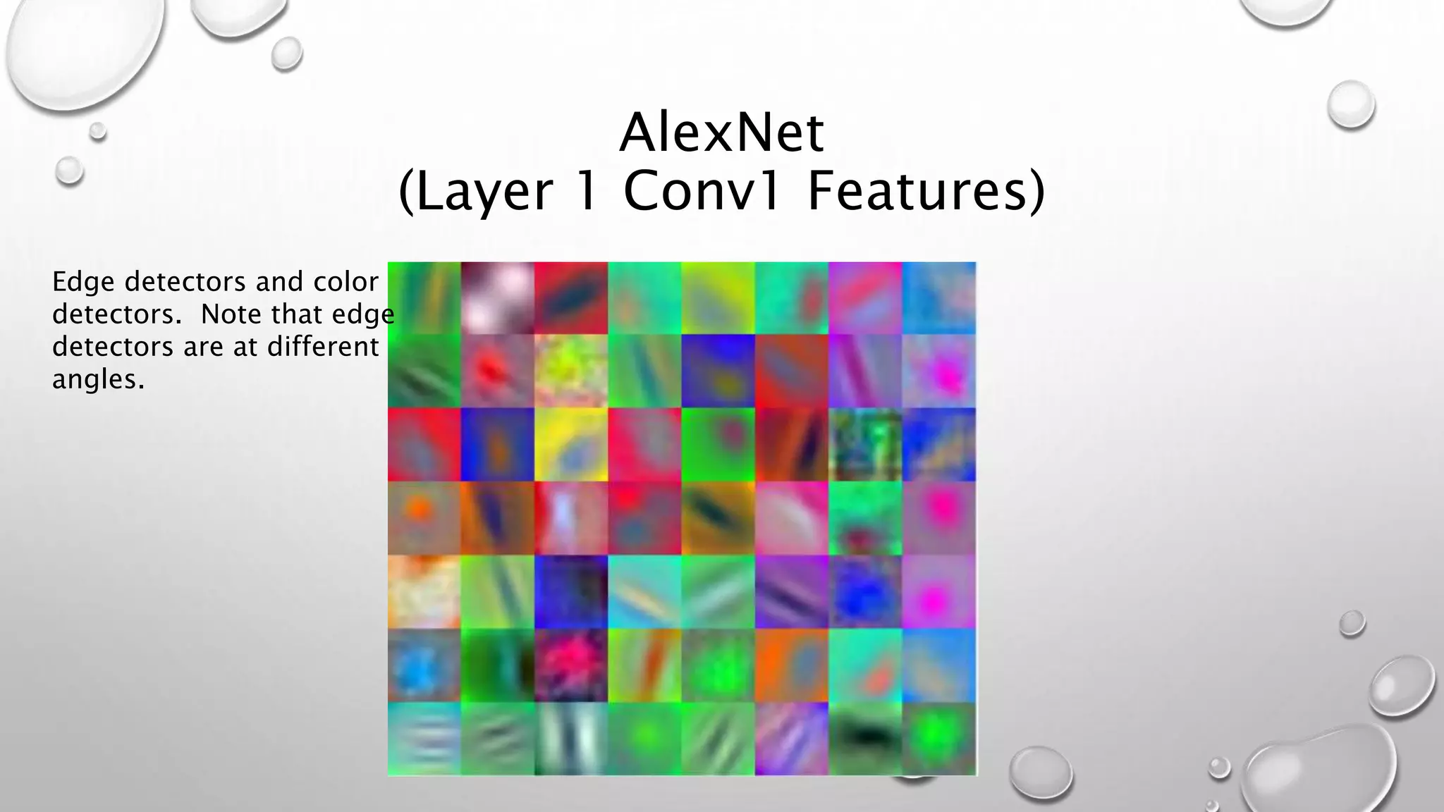
AlexNet
(Layer 1 Conv1 Features)
Edge detectors and color
detectors. Note that edge
detectors are at different
angles.

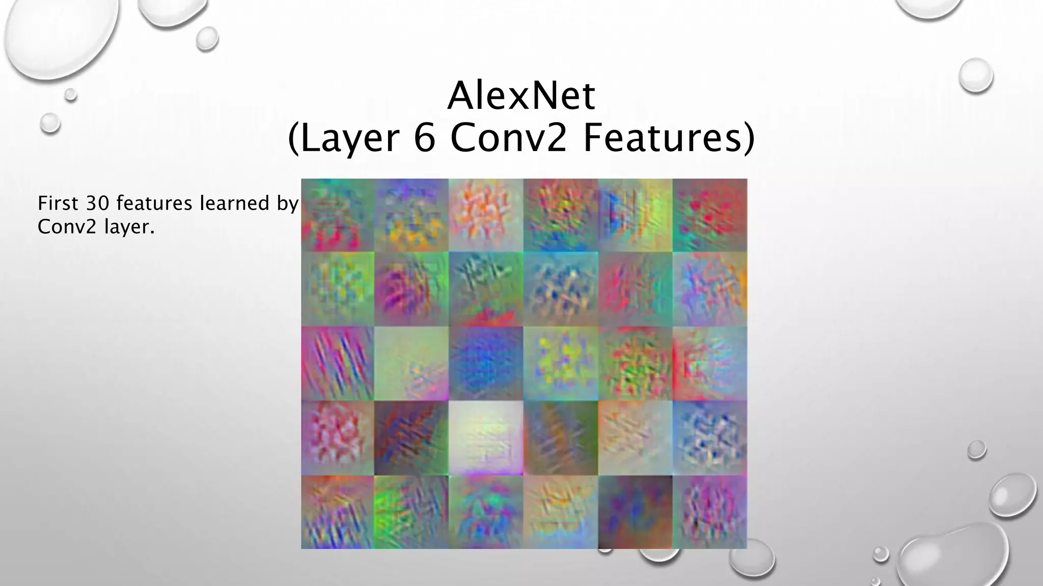
AlexNet
(Layer 6 Conv2 Features)
First 30 features learned by
Conv2 layer.

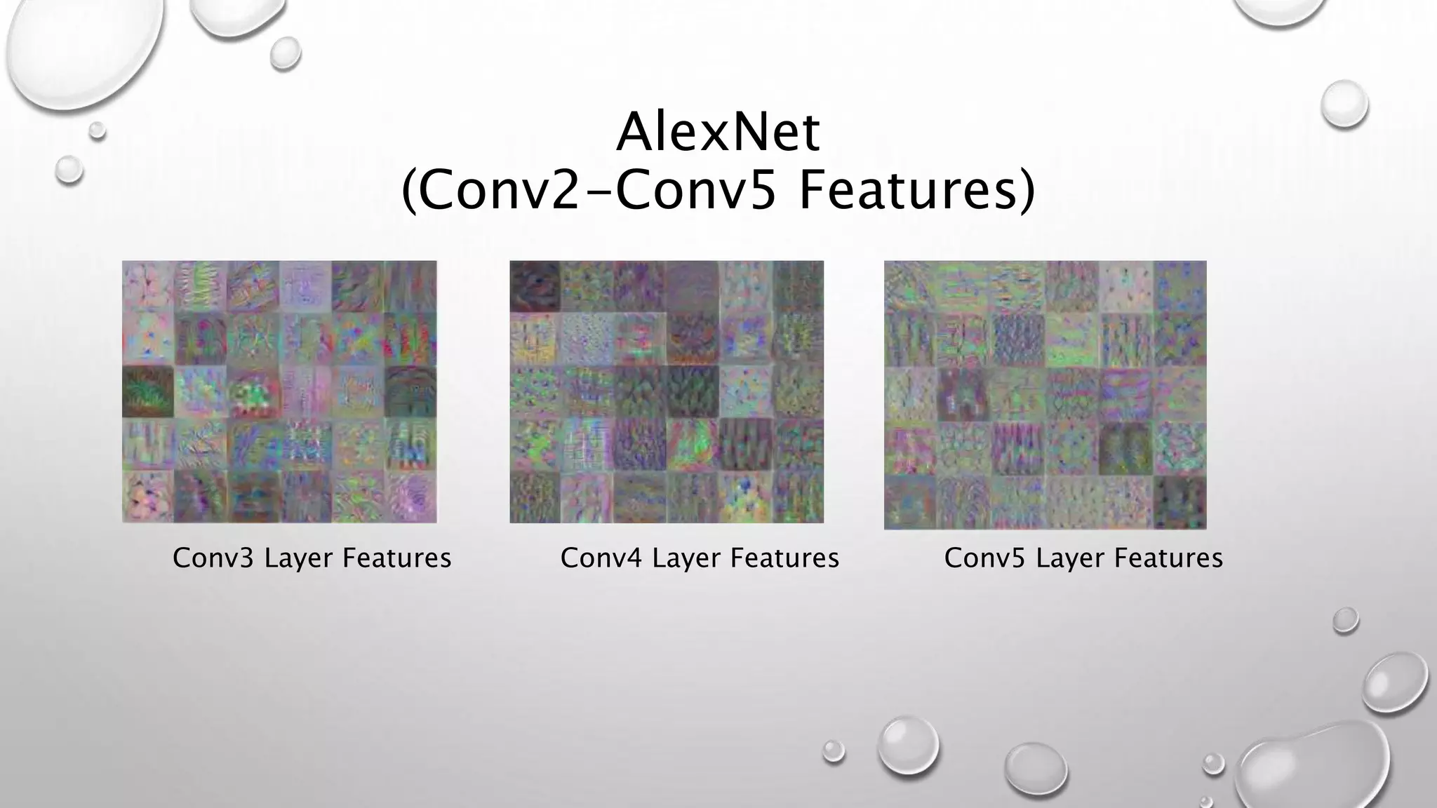
AlexNet
(Conv2-Conv5 Features)
Conv3 Layer Features Conv4 Layer Features Conv5 Layer Features

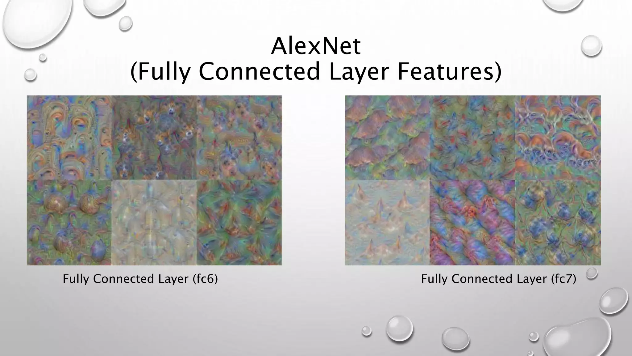
AlexNet
(Fully Connected Layer Features)
Fully Connected Layer (fc6) Fully Connected Layer (fc7)

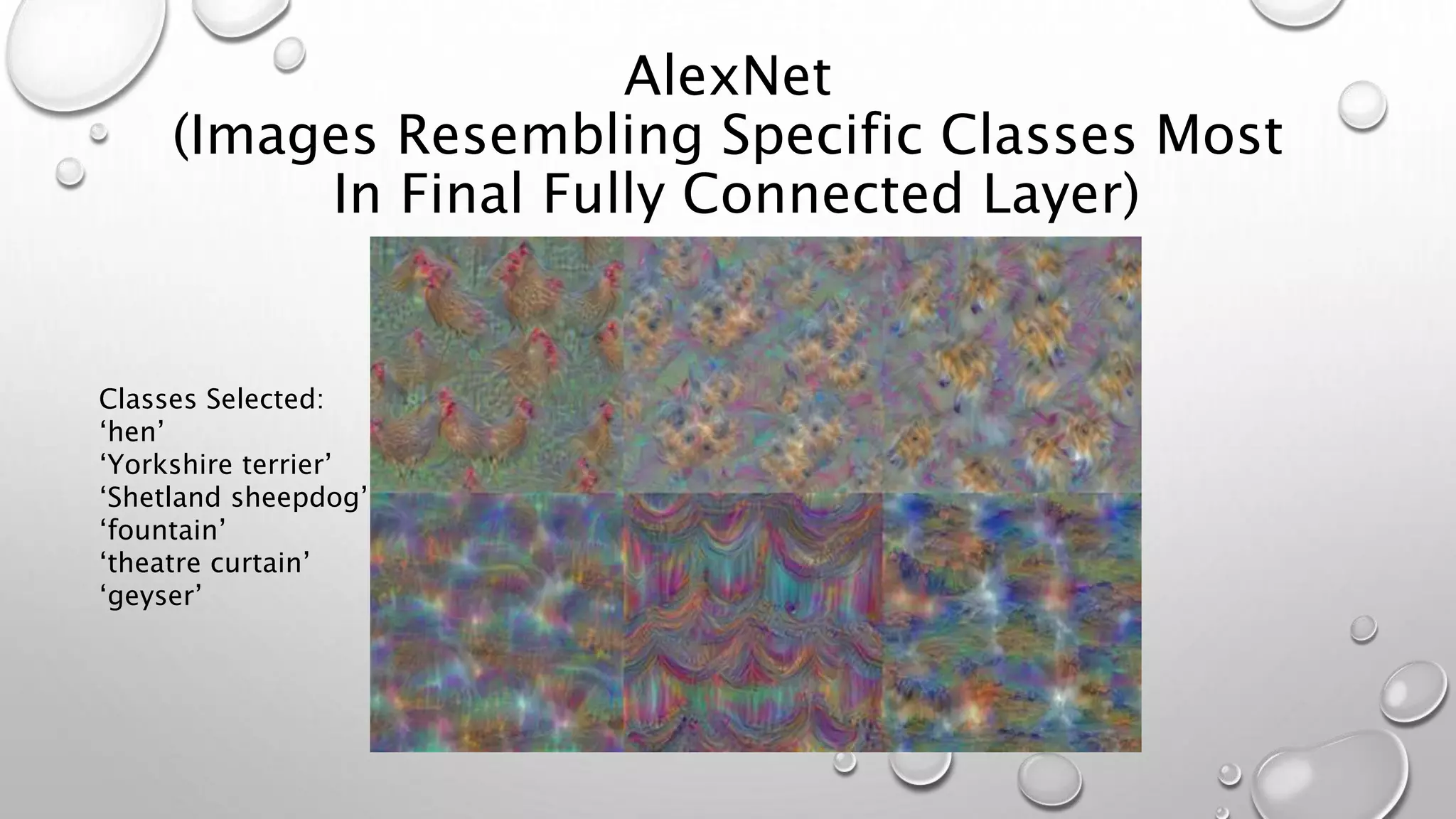
AlexNet
(Images Resembling Specific Classes Most
In Final Fully Connected Layer)
Classes Selected:
‘hen’
‘Yorkshire terrier’
‘Shetland sheepdog’
‘fountain’
‘theatre curtain’
‘geyser’

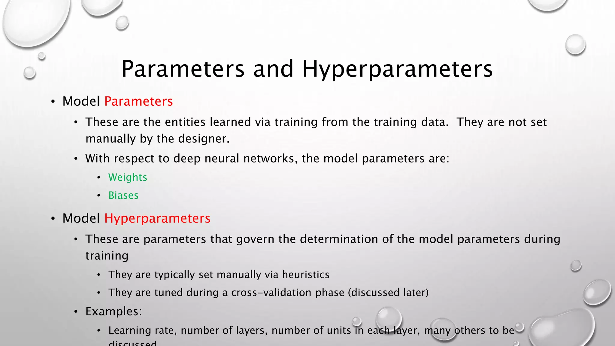
Parameters and Hyperparameters
• Model Parameters
• These are the entities learned via training from the training data. They are not set
manually by the designer.
• With respect to deep neural networks, the model parameters are:
• Weights
• Biases
• Model Hyperparameters
• These are parameters that govern the determination of the model parameters during
training
• They are typically set manually via heuristics
• They are tuned during a cross-validation phase (discussed later)
• Examples:
• Learning rate, number of layers, number of units in each layer, many others to be

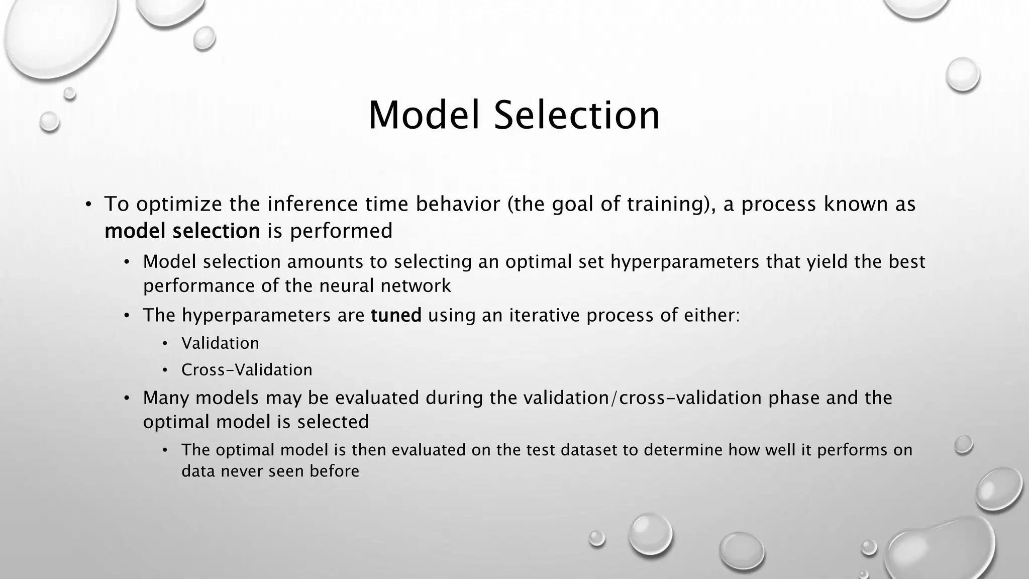
Model Selection
• To optimize the inference time behavior (the goal of training), a process known as
model selection is performed
• Model selection amounts to selecting an optimal set hyperparameters that yield the best
performance of the neural network
• The hyperparameters are tuned using an iterative process of either:
• Validation
• Cross-Validation
• Many models may be evaluated during the validation/cross-validation phase and the
optimal model is selected
• The optimal model is then evaluated on the test dataset to determine how well it performs on
data never seen before

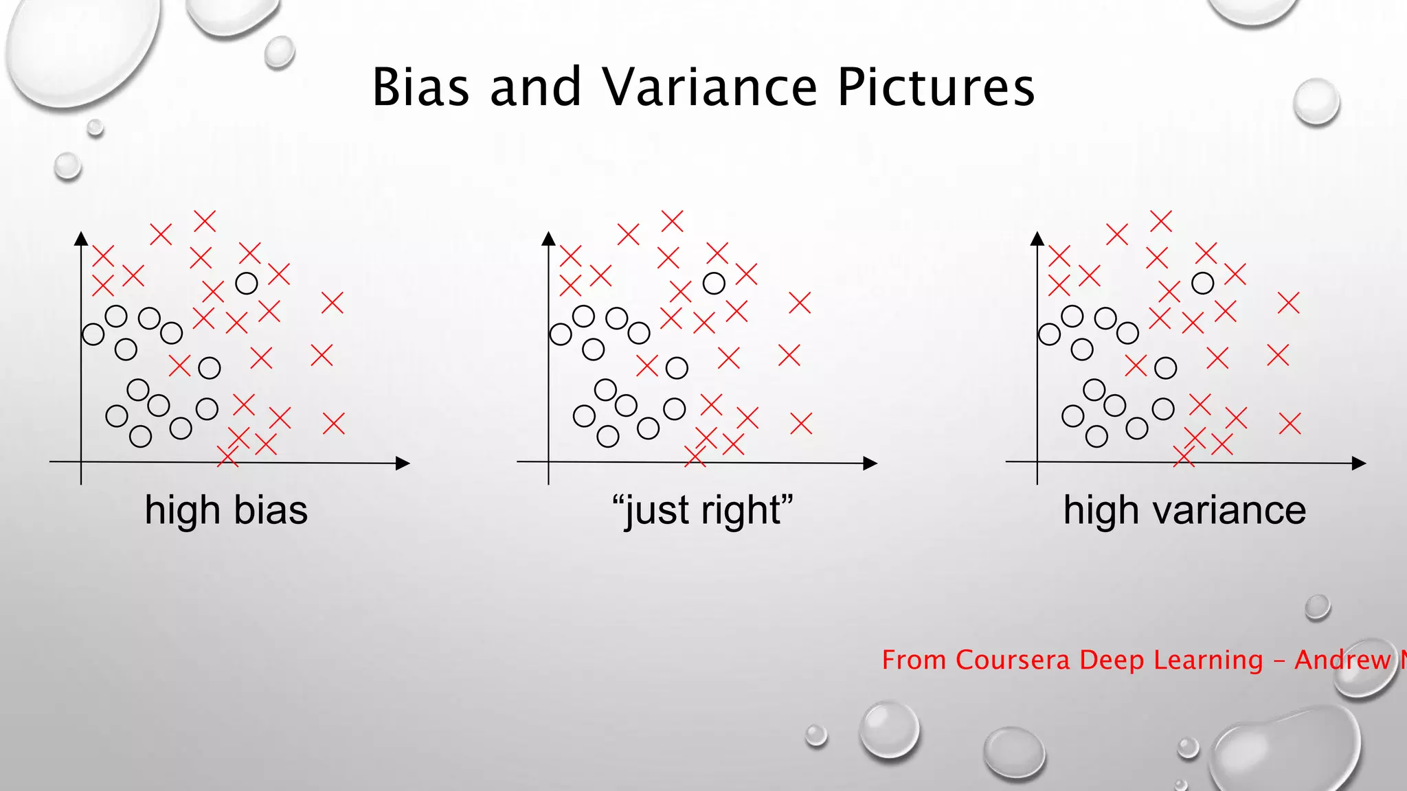
Bias and Variance Pictures
From Coursera Deep Learning – Andrew N
high bias “just right” high variance

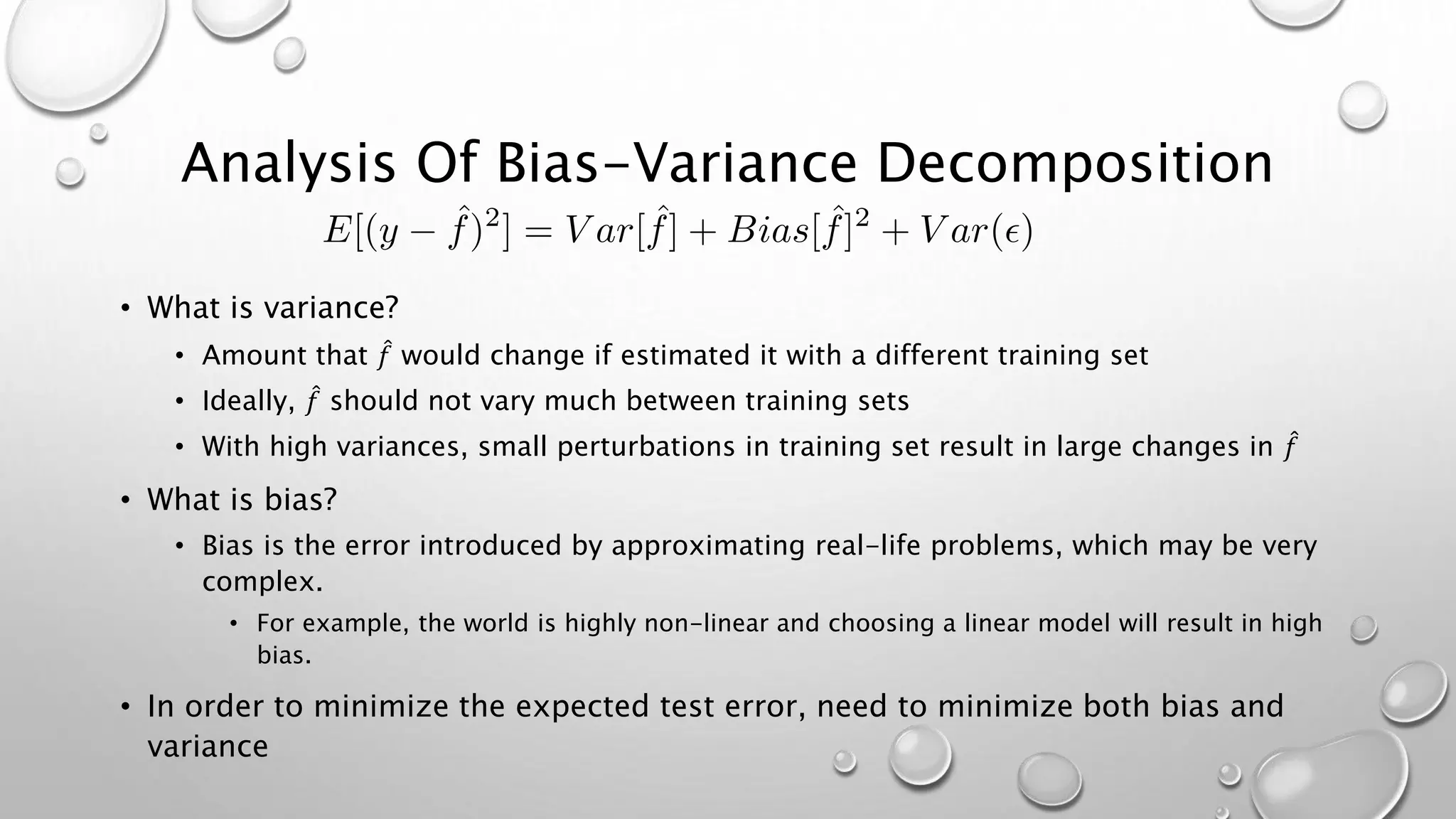
Analysis Of Bias-Variance Decomposition
• What is variance?
• Amount that 𝑓 would change if estimated it with a different training set
• Ideally, 𝑓 should not vary much between training sets
• With high variances, small perturbations in training set result in large changes in 𝑓
• What is bias?
• Bias is the error introduced by approximating real-life problems, which may be very
complex.
• For example, the world is highly non-linear and choosing a linear model will result in high
bias.
• In order to minimize the expected test error, need to minimize both bias and
variance

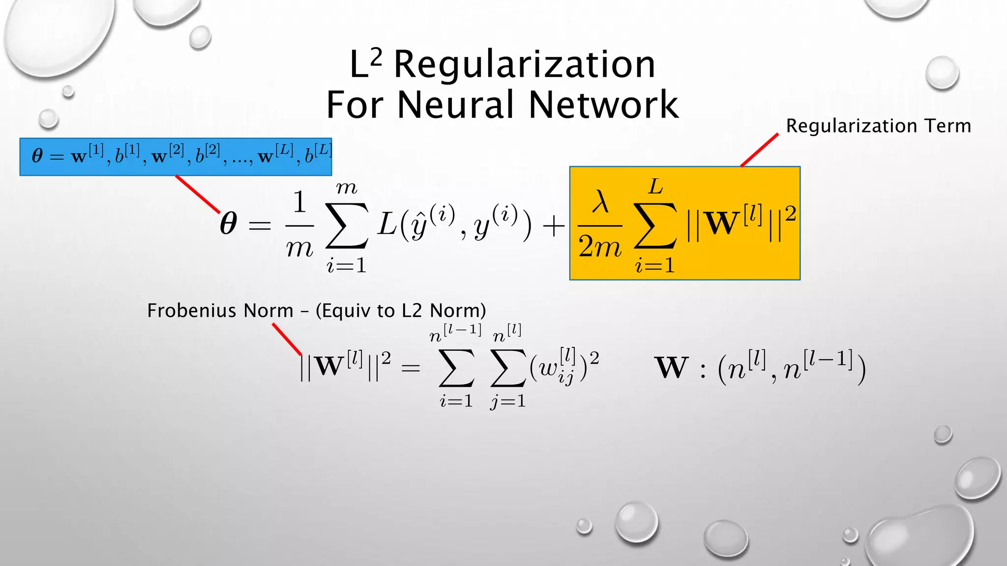
L2 Regularization
For Neural Network Regularization Term
Frobenius Norm – (Equiv to L2 Norm)

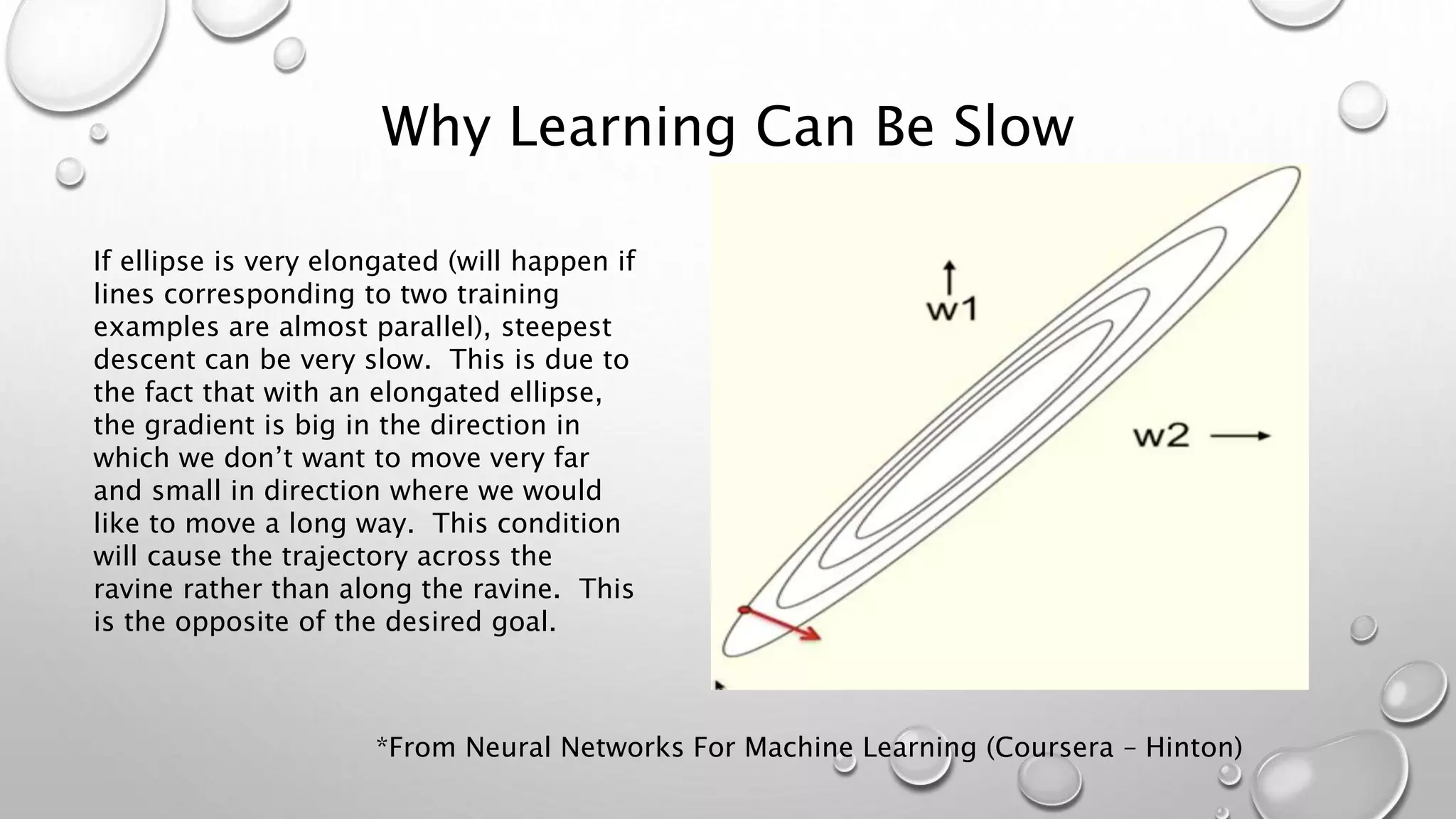
Why Learning Can Be Slow
If ellipse is very elongated (will happen if
lines corresponding to two training
examples are almost parallel), steepest
descent can be very slow. This is due to
the fact that with an elongated ellipse,
the gradient is big in the direction in
which we don’t want to move very far
and small in direction where we would
like to move a long way. This condition
will cause the trajectory across the
ravine rather than along the ravine. This
is the opposite of the desired goal.
*From Neural Networks For Machine Learning (Coursera – Hinton)

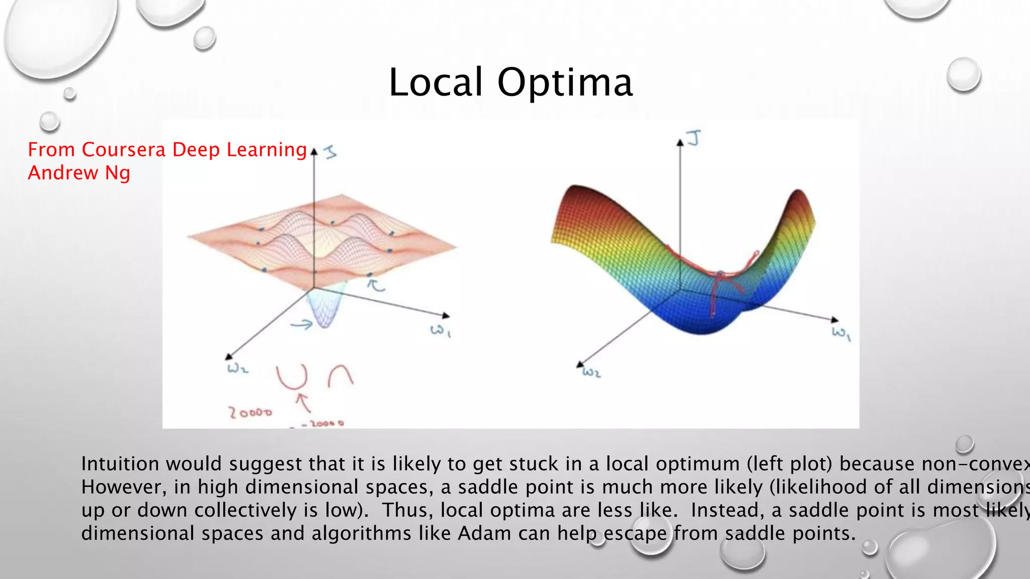
Local Optima
Intuition would suggest that it is likely to get stuck in a local optimum (left plot) because non-convex
However, in high dimensional spaces, a saddle point is much more likely (likelihood of all dimensions
up or down collectively is low). Thus, local optima are less like. Instead, a saddle point is most likely
dimensional spaces and algorithms like Adam can help escape from saddle points.
From Coursera Deep Learning
Andrew Ng

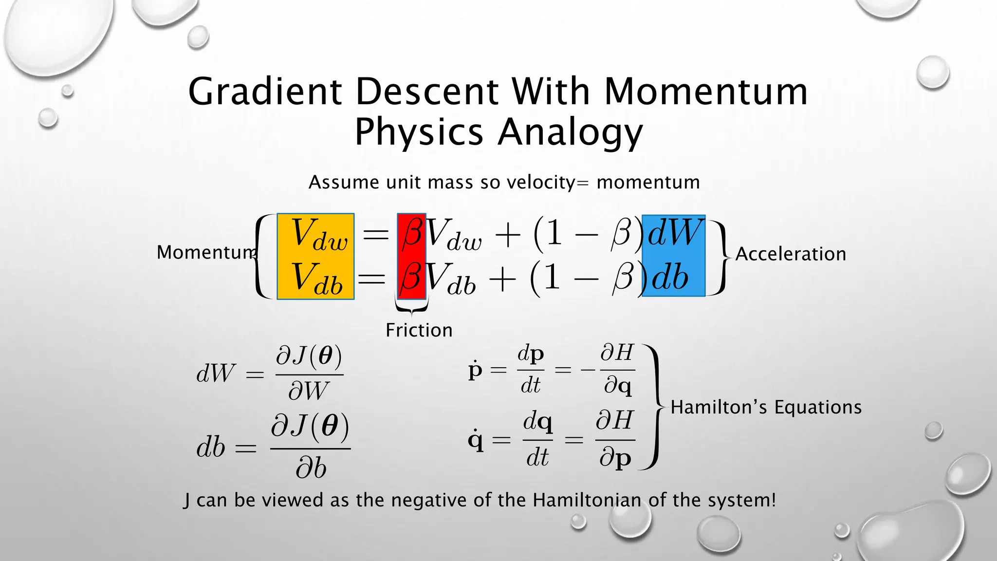
Gradient Descent With Momentum
Physics Analogy
Acceleration
Assume unit mass so velocity= momentum
Momentum
Friction
J can be viewed as the negative of the Hamiltonian of the system!
Hamilton’s Equations

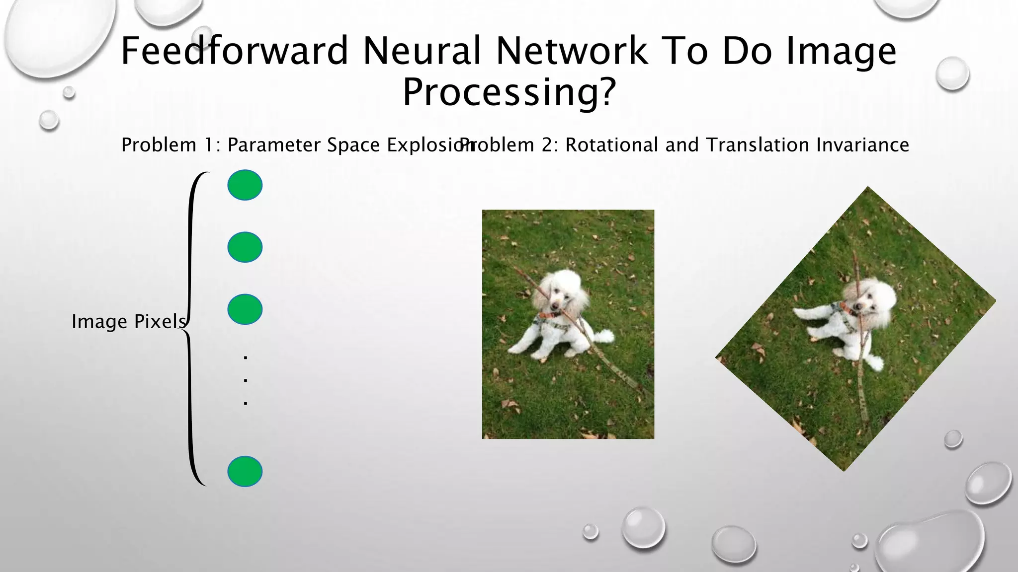
Feedforward Neural Network To Do Image
Processing?
.
.
.
Image Pixels
Problem 1: Parameter Space ExplosionProblem 2: Rotational and Translation Invariance

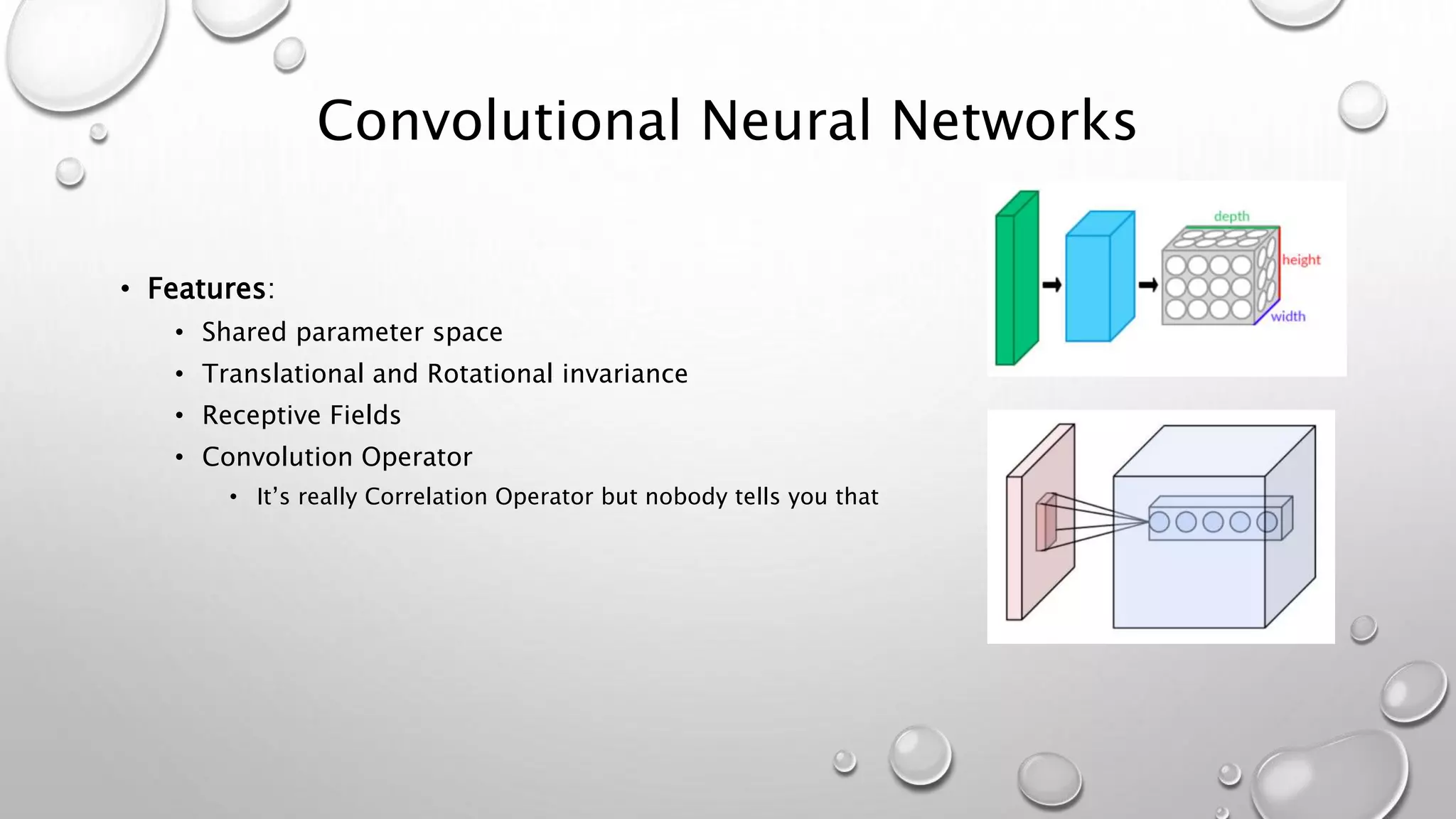
Convolutional Neural Networks
• Features:
• Shared parameter space
• Translational and Rotational invariance
• Receptive Fields
• Convolution Operator
• It’s really Correlation Operator but nobody tells you that

What about Memory?
• Our neurons cannot remember anything
• What about correlations to the past?
• What about correlations to the future?
• Solution: Recurrent Neural Networks
• Carry Hidden State
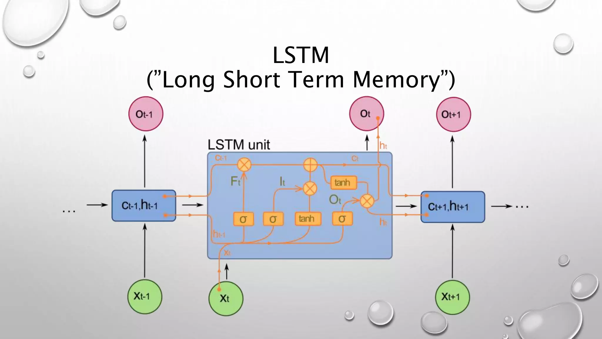
• LSTMs (”Long Short Term Memory”) are one example

LSTM
(”Long Short Term Memory”)

What is TensorFlow?
• TensorFlow is a machine learning software framework based on the dataflow programming
paradigm
• A software framework is a reusable software environment that provides generic functionality that can
be selectively changed by additional user-write code, thus providing application specific software.
• Dataflow Programming
• Programming paradigm that models a program as a directed graph of the data flowing between
operations
• Data moves between nodes of the graph
• Imagine an assembly line with data moving between workers (data in motion)
• No hidden state to manage
• Contrast sequential programming:
• Data is at rest
• Requires state handling code

TensorFlow Graphs And Sessions
• TensorFlow is modeled on the Dataflow paradigm
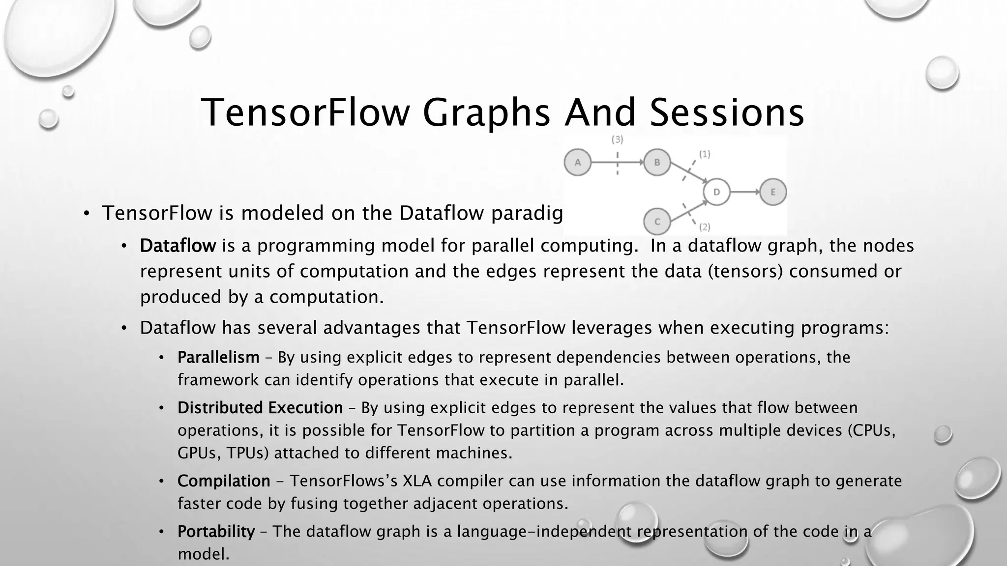
• Dataflow is a programming model for parallel computing. In a dataflow graph, the nodes
represent units of computation and the edges represent the data (tensors) consumed or
produced by a computation.
• Dataflow has several advantages that TensorFlow leverages when executing programs:
• Parallelism – By using explicit edges to represent dependencies between operations, the
framework can identify operations that execute in parallel.
• Distributed Execution – By using explicit edges to represent the values that flow between
operations, it is possible for TensorFlow to partition a program across multiple devices (CPUs,
GPUs, TPUs) attached to different machines.
• Compilation - TensorFlows’s XLA compiler can use information the dataflow graph to generate
faster code by fusing together adjacent operations.
• Portability – The dataflow graph is a language-independent representation of the code in a
model.

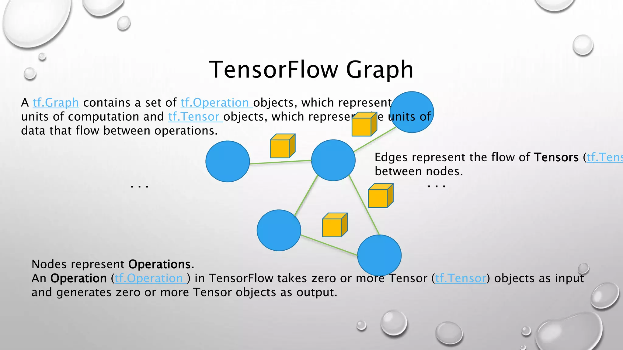
TensorFlow Graph
Nodes represent Operations.
An Operation (tf.Operation ) in TensorFlow takes zero or more Tensor (tf.Tensor) objects as input
and generates zero or more Tensor objects as output.
. . .. . .
Edges represent the flow of Tensors (tf.Tens
between nodes.
A tf.Graph contains a set of tf.Operation objects, which represent
units of computation and tf.Tensor objects, which represent the units of
data that flow between operations.

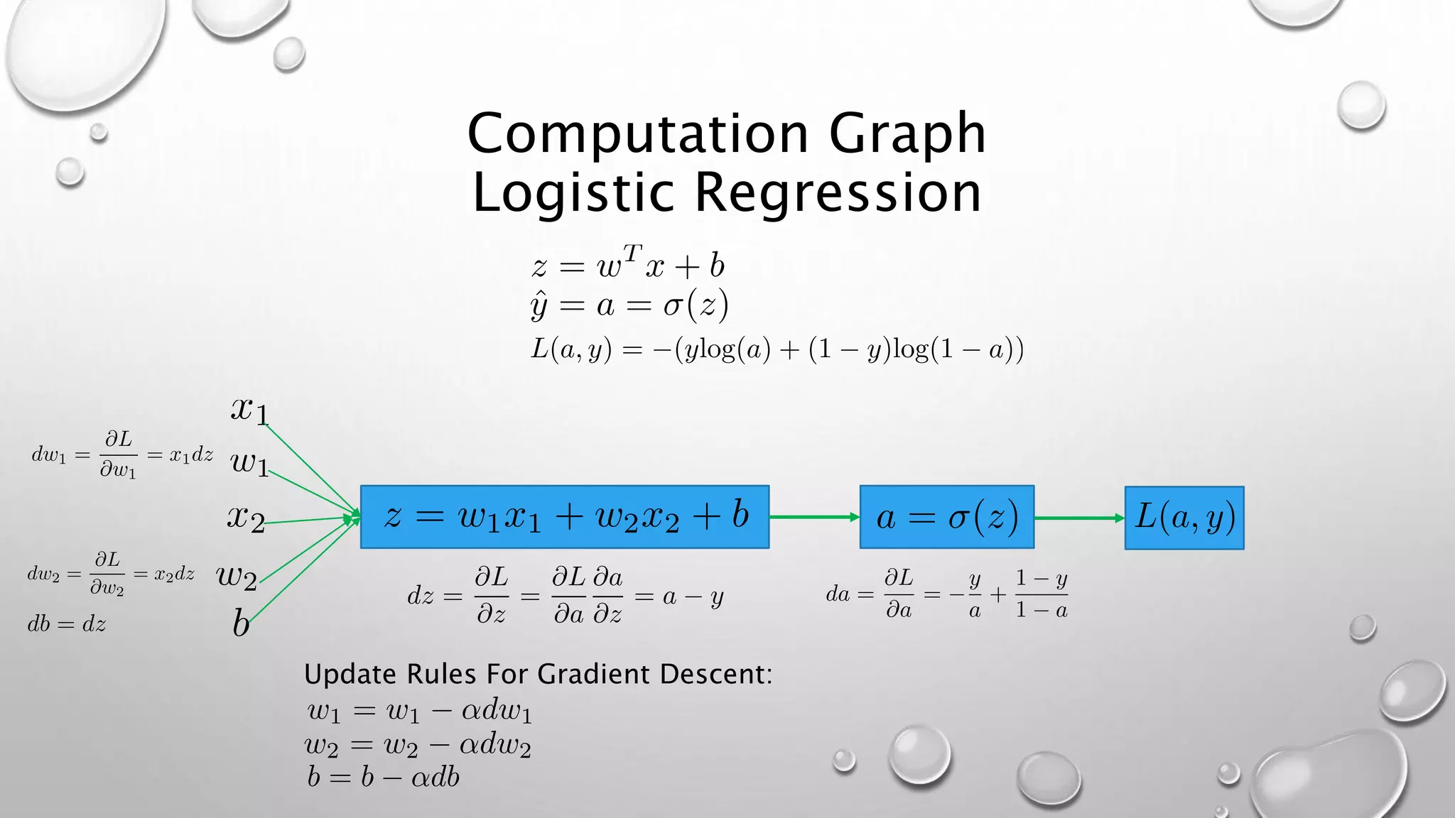
Computation Graph
Logistic Regression
Update Rules For Gradient Descent:

Deep Learning Sample Class (Jon Lederman)

More Related Content

What's hot

Similar to Deep Learning Sample Class (Jon Lederman)

Recently uploaded

Deep Learning Sample Class (Jon Lederman)