Definition
Prof. K. Adisesha2
⚫Data: Collection of raw facts.
⚫Data structure is representation of the
logical relationship existing between
individual elements of data.
⚫Data structure is a specialized format for
organizing and storing data in memory that
considers not only the elements stored but
also their relationship to each other.
3.
Introduction
Prof. K. Adisesha3
⚫Data structure affects the design of both
structural & functional aspects of a
program.
Program=algorithm + Data Structure
⚫You know that a algorithm is a step by step
procedure to solve a particular function.
4.
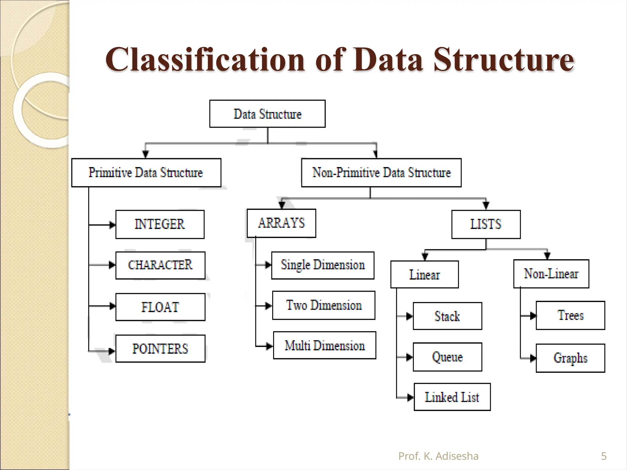
Classification of DataStructure
Prof. K. Adisesha 4
⚫Data structure are normally divided
into two broad categories:
◦ Primitive Data Structure
◦ Non-Primitive Data Structure
Primitive Data Structure
Prof.K. Adisesha 6
⚫There are basic structures and directly
operated upon by the machine
instructions.
⚫Data structures that are directly operated
upon the machine-level instructions are
known as primitive data structures.
⚫Integer, Floating-point number, Character
constants, string constants, pointers etc,
fall in this category.
7.
Primitive Data Structure
Prof.K. Adisesha 7
⚫The most commonly used operation on
data structure are broadly categorized into
following types:
◦ Create
◦ Selection
◦ Updating
◦ Destroy or Delete
8.
Non-Primitive Data Structure
Prof.K. Adisesha 8
⚫There are more sophisticated
data structures.
⚫ The Data structures that are derived from the
primitive data structures are called Non-
primitive data structure.
⚫The non-primitive data structures
emphasize on structuring of a group of
homogeneous (same type) or
heterogeneous (different type) data items.
9.
Non-Primitive Data Structure
Prof.K. Adisesha 9
Linear Data structures:
◦ Linear Data structures are kind of data structure that has homogeneous
elements.
◦ The data structure in which elements are in a sequence and form a liner
series.
◦ Linear data structures are very easy to implement, since the memory of
the computer is also organized in a linear fashion.
◦ Some commonly used linear data structures are Stack, Queue and
Linked
Lists.
Non-Linear Data structures:
◦ A Non-Linear Data structures is a data structure in which data item is
connected to several other data items.
◦ Non-Linear data structure may exhibit either a hierarchical relationship or
parent child relationship.
◦ The data elements are not arranged in a sequential structure.
◦ The different non-linear data structures are trees and graphs.
10.
Non-Primitive Data Structure
Prof.K. Adisesha 10
⚫The most commonly used operation on
data structure are broadly categorized into
following types:
◦ Traversal
◦ Insertion
◦ Selection
◦ Searching
◦ Sorting
◦ Merging
◦ Destroy or Delete
11.
Different between them
Prof.K. Adisesha 11
⚫A primitive data structure is generally a
basic structure that is usually built into
the language, such as an integer, a float.
⚫A non-primitive data structure is built
out of primitive data structures linked
together in meaningful ways, such as a
or a linked-list, binary search tree, AVL
Tree, graph etc.
12.
Description of various
DataStructures :
Arrays
Prof. K. Adisesha 12
⚫An array is defined as a set of finite
number of homogeneous elements
or same data items.
⚫It means an array can contain one type of
data only, either all integer, all float-
point number or all character.
13.
One dimensional array:
Prof.K. Adisesha 13
⚫ An array with only one row or column is called one-dimensional
array.
⚫ It is finite collection of n number of elements of same type such
that:
◦ can be referred by indexing.
◦ The syntax Elements are stored in continuous locations.
◦ Elements x to define one-dimensional array is:
⚫ Syntax: Datatype Array_Name [Size];
⚫ Where,
Datatype : Type of value it can store (Example: int, char, float)
Array_Name: To identify the array.
⚫ Size : The maximum number of elements that the array can hold.
14.
Arrays
Prof. K. Adisesha14
⚫Simply, declaration of array is as follows:
int arr[10]
⚫Where int specifies the data type or type
of elements arrays stores.
⚫“arr” is the name of array & the number
specified inside the square brackets is the
number of elements an array can store, this
is also called sized or length of array.
15.
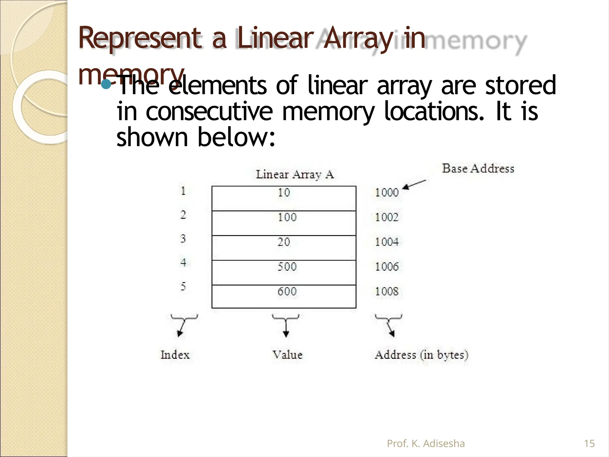
Represent a LinearArray in
memory
⚫The elements of linear array are stored
in consecutive memory locations. It is
shown below:
Prof. K. Adisesha 15
16.
Arrays
Prof. K. Adisesha16
◦ The elements of array will always be stored in the
consecutive (continues) memory location.
◦ The number of elements that can be stored in an
array, that is the size of array or its length is given
by the following equation:
(Upperbound-lowerbound)+1
◦ For the above array it would be (9-0)+1=10,where 0
is the lower bound of array and 9 is the upper bound
of array.
◦ Array can always be read or written through loop.
For(i=0;i<=9;i++)
{ scanf(“%d”,&arr[i]);
printf(“%d”,arr[i]); }
17.
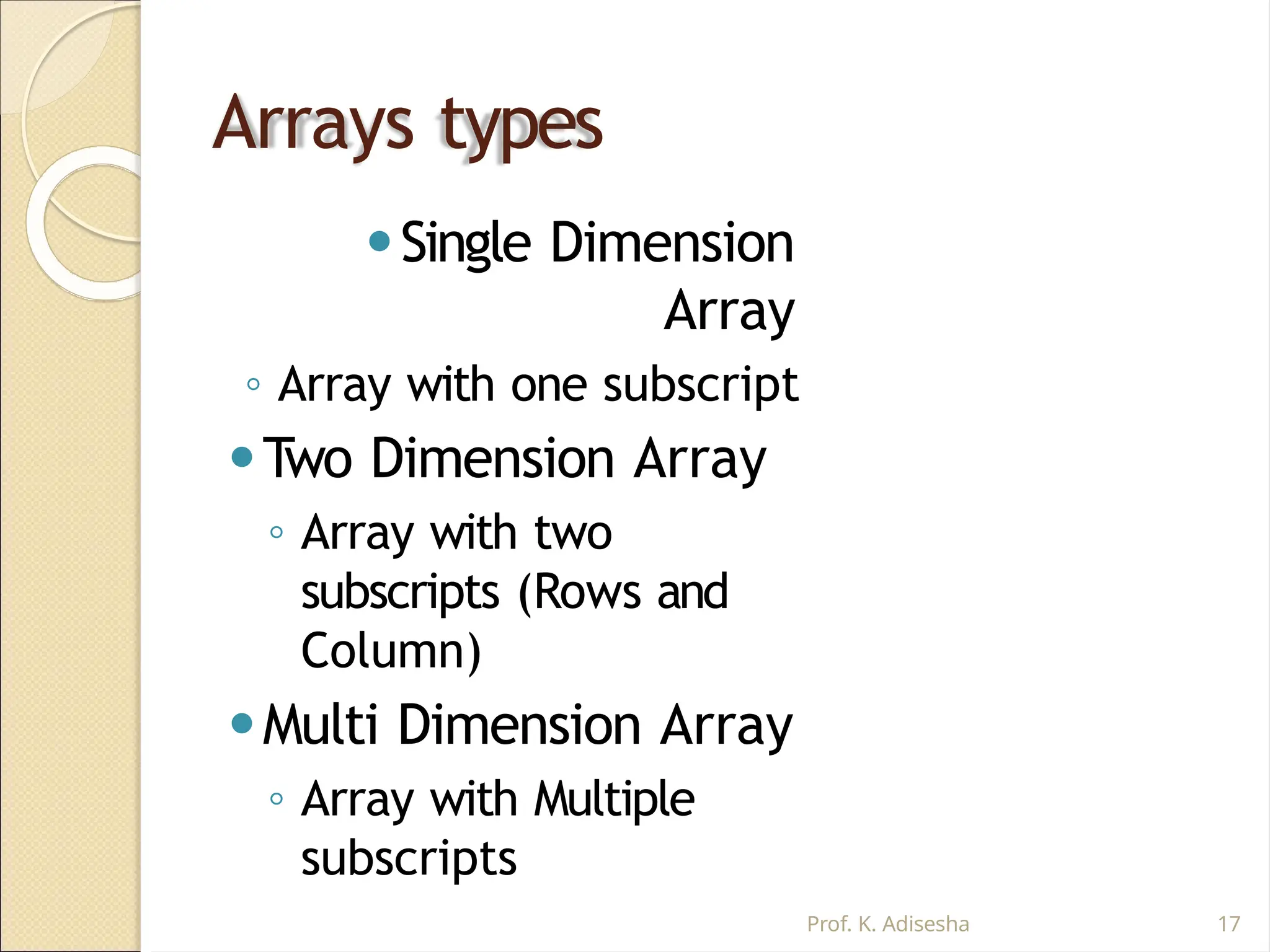
Arrays types
Prof. K.Adisesha 17
⚫Single Dimension
Array
◦ Array with one subscript
⚫Two Dimension Array
◦ Array with two
subscripts (Rows and
Column)
⚫Multi Dimension Array
◦ Array with Multiple
subscripts
18.
Basic operations ofArrays
Prof. K. Adisesha 18
⚫Some common operation performed
on array are:
◦ Traversing
◦ Searching
◦ Insertion
◦ Deletion
◦ Sorting
◦ Merging
19.
Traversing Arrays
⚫ Traversing:It is used to access each data item exactly once
so
that it can be processed.
E.g.
We have linear array A as below:
⚫ 1 2 3 4 5
⚫ 10 20 30 40 50
Here we will start from beginning and will go till last element
and during this process we will access value of each element
exactly once as below:
A [1] = 10
A [2] = 20
A [3] = 30
A [4] = 40
A [5] = 50
Prof. K. Adisesha 19
20.
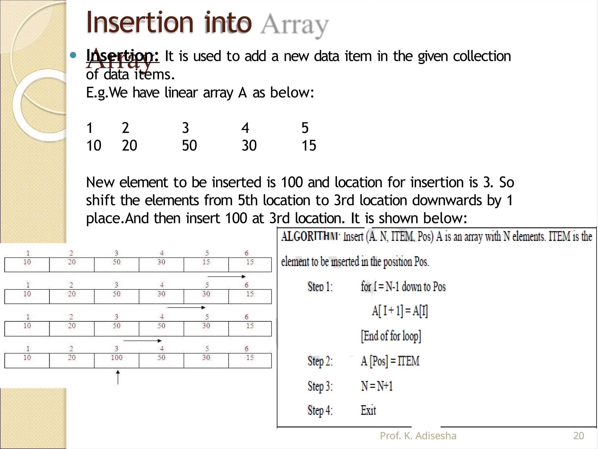
Insertion into
Array
⚫ Insertion:It is used to add a new data item in the given collection
of data items.
E.g.We have linear array A as below:
1 2 3 4 5
10 20 50 30 15
New element to be inserted is 100 and location for insertion is 3. So
shift the elements from 5th location to 3rd location downwards by 1
place.And then insert 100 at 3rd location. It is shown below:
Prof. K. Adisesha 20
21.
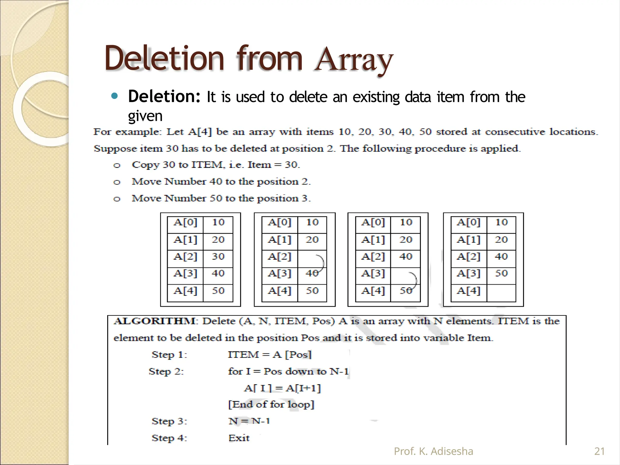
Deletion from Array
⚫Deletion: It is used to delete an existing data item from the
given
collection of data items.
Prof. K. Adisesha 21
22.
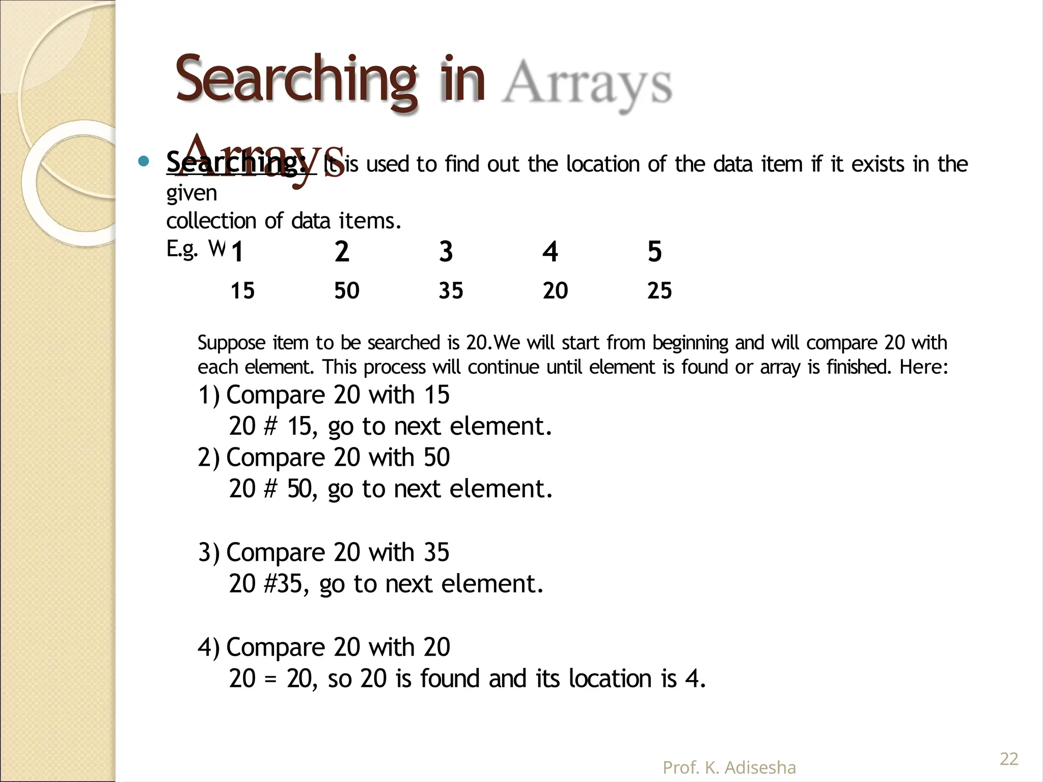
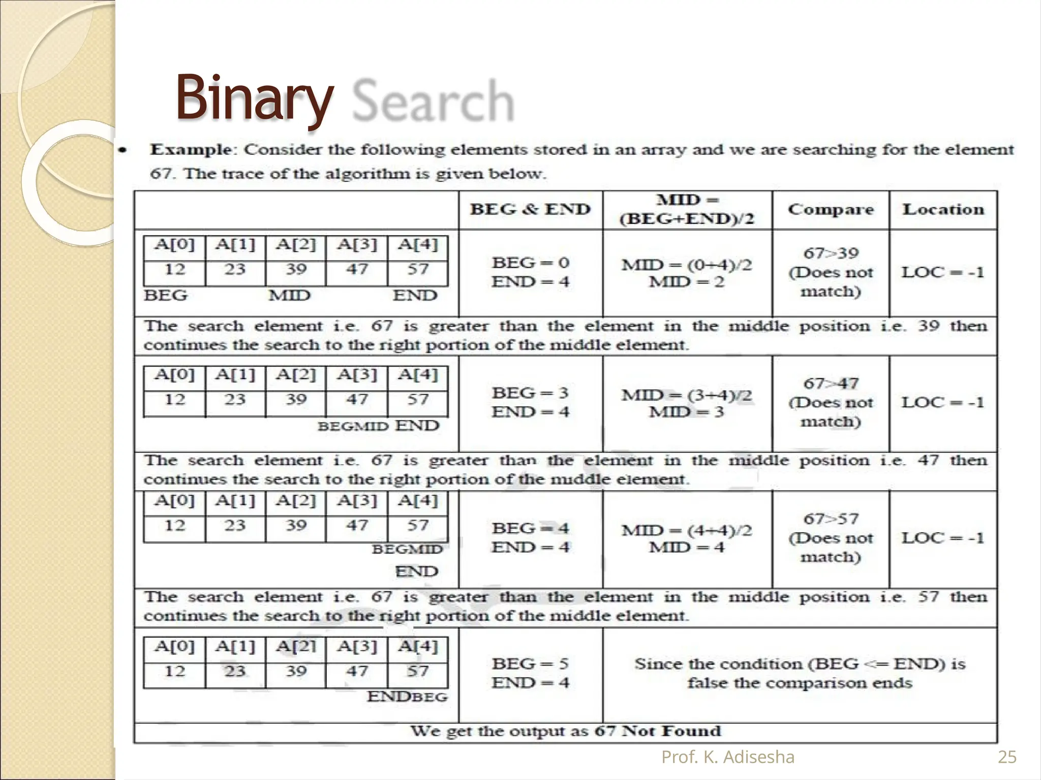
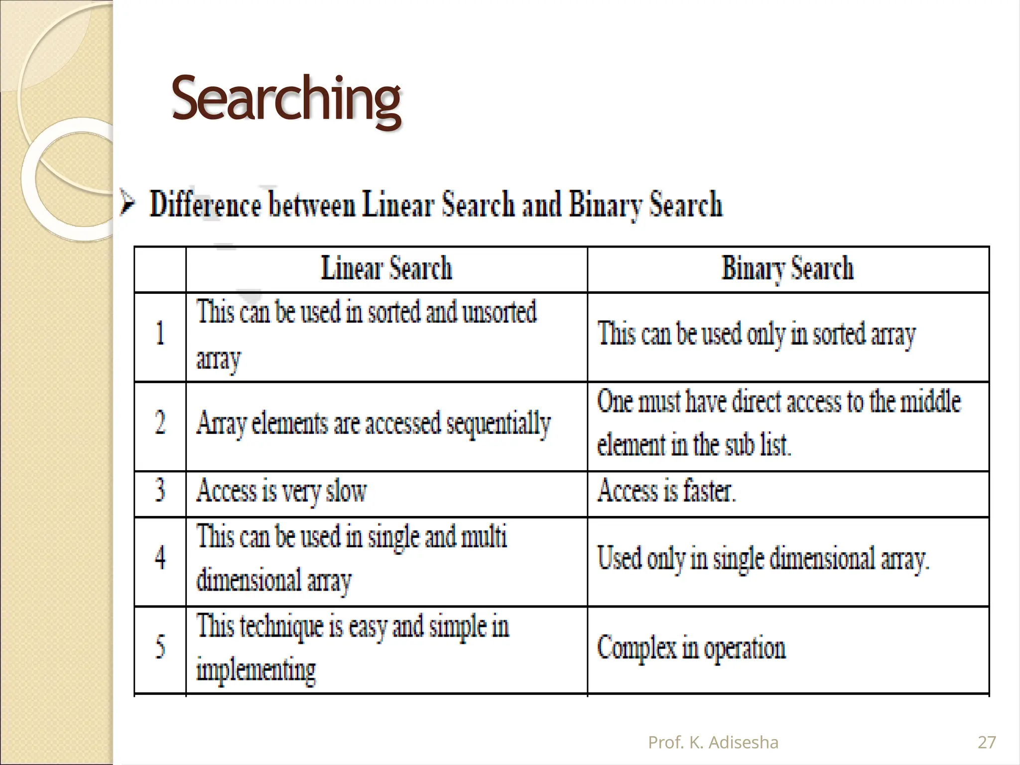
Searching in
Arrays
22
Prof. K.Adisesha
⚫ Searching: It is used to find out the location of the data item if it exists in the
given
collection of data items.
E.g. We have linear array A as below:
1 2 3 4 5
15 50 35 20 25
Suppose item to be searched is 20.We will start from beginning and will compare 20 with
each element. This process will continue until element is found or array is finished. Here:
1) Compare 20 with 15
20 # 15, go to next element.
2) Compare 20 with 50
20 # 50, go to next element.
3) Compare 20 with 35
20 #35, go to next element.
4) Compare 20 with 20
20 = 20, so 20 is found and its location is 4.
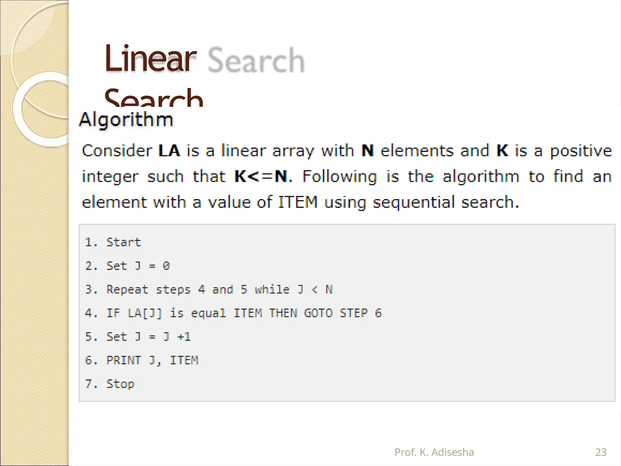
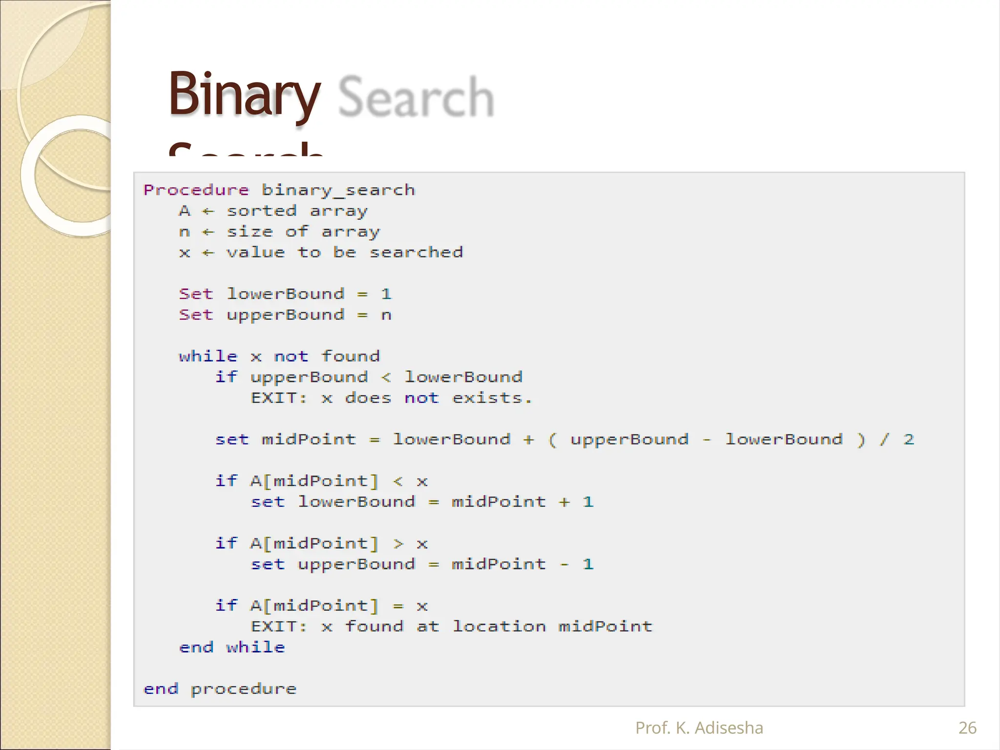
⚫ The binarysearch
algorithm can be used with
only sorted list of
elements.
⚫ Binary Search first divides
a large array into two
smaller sub-arrays and
then recursively operate
the sub-arrays.
⚫ Binary Search basically
reduces the search space to
half at each step
Binary
Search
Prof. K. Adisesha 24
Insertion Sort
⚫ ALGORITHM:Insertion Sort (A, N) A is an array with
N
unsorted elements.
◦ Step 1: for I=1 to N-1
◦ Step 2: J = I
While(J >= 1)
if ( A[J] < A[J-1] ) then
T
emp = A[J];
A[J] = A[J-1];
A[J-1] =
T
emp;
[End if]
J = J-1
[End of While
loop] [End of For
loop] Prof. K. Adisesha 29
30.
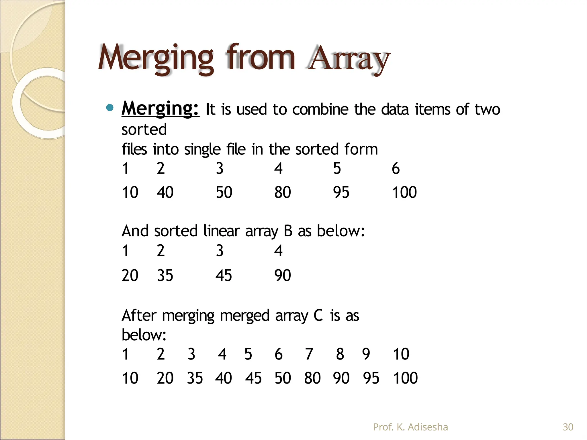
Merging from Array
Prof.K. Adisesha 30
⚫ Merging: It is used to combine the data items of two
sorted
files into single file in the sorted form
We have sorted linear array A as below:
1 2 3 4 5 6
10 40 50 80 95 100
And sorted linear array B as below:
1 2 3 4
20 35 45 90
After merging merged array C is as
below:
1 2 3 4 5 6 7 8 9 10
10 20 35 40 45 50 80 90 95 100
31.
Two dimensional
array
Prof. K.Adisesha 31
⚫ A two dimensional array is a collection of elements and
each element is identified by a pair of subscripts. ( A[3] [3]
)
⚫ The elements are stored in continuous memory
locations.
⚫ The elements of two-dimensional array as rows and
columns.
⚫ The number of rows and columns in a matrix is
called as
the order of the matrix and denoted as mxn.
⚫ The number of elements can be obtained by
multiplying
number of rows and number of columns.
A[0] A[1] A[2]
A[0] 10 20 30
A[1] 40 50 60
A[2] 70 80 90
32.
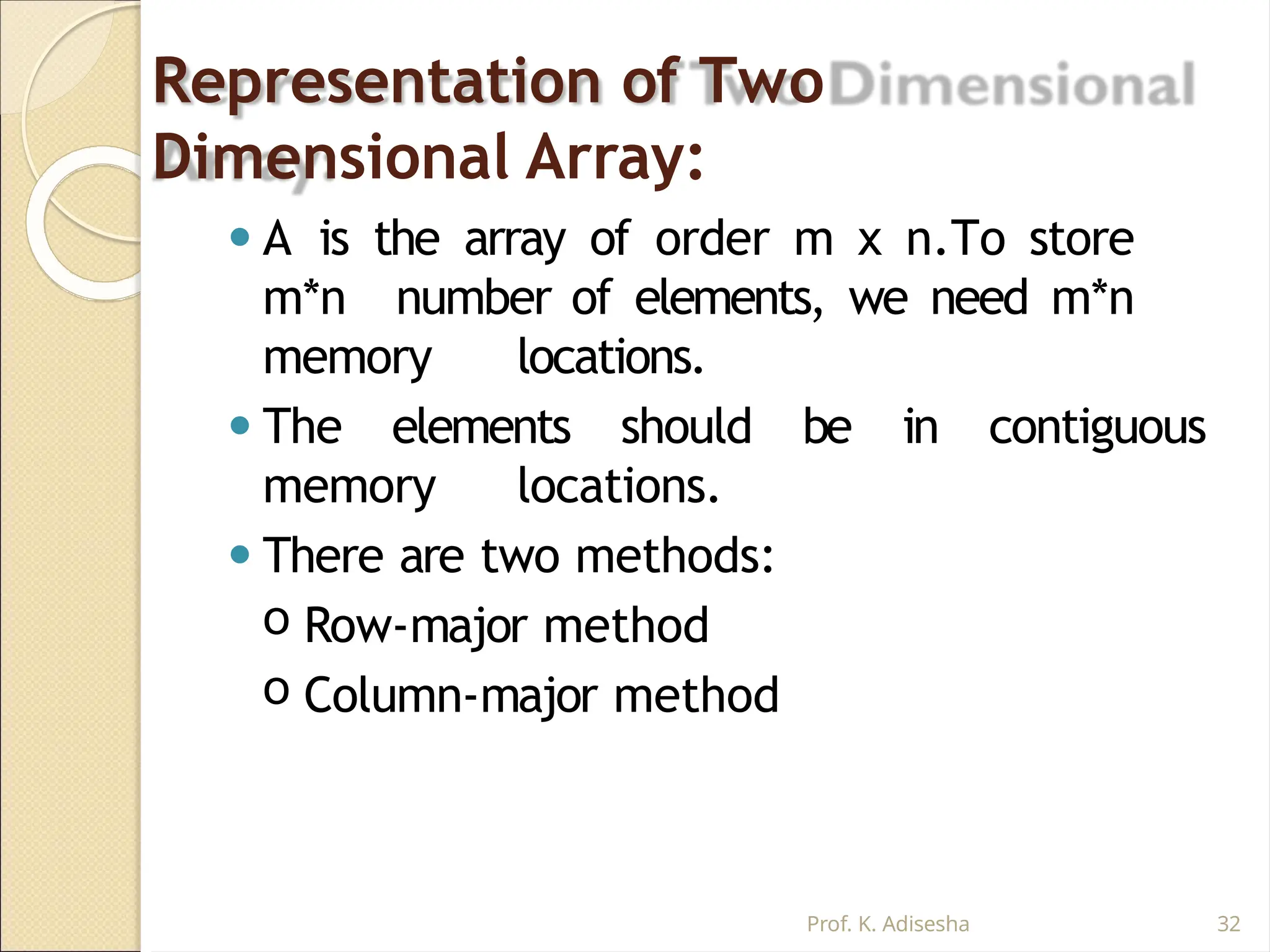
Representation of Two
DimensionalArray:
Prof. K. Adisesha 32
⚫ A is the array of order m x n.To store
m*n number of elements, we need m*n
memory locations.
⚫ The elements should be in contiguous
memory locations.
⚫ There are two methods:
o Row-major method
o Column-major method
33.
Two Dimensional
Array:
Prof. K.Adisesha 33
⚫ Row-Major Method: All the first-row elements are stored
in sequential memory locations and then all the second-row
elements are stored and so on. Ex: A[Row][Col]
⚫ Column-Major Method: All the first column elements are
stored in sequential memory locations and then all the
second- column elements are stored and so on. Ex: A [Col]
[Row] 1000 10 A[0][0]
1002 20 A[0][1]
1004 30 A[0][2]
1006 40 A[1][0]
1008 50 A[1][1]
1010 60 A[1][2]
1012 70 A[2][0]
1014 80 A[2][1]
1016 90 A[2][2]
Row-Major Method
1000 10 A[0][0]
1002 40 A[1][0]
1004 70 A[2][0]
1006 20 A[0][1]
1008 50 A[1][1]
1010 80 A[2][1]
1012 30 A[0][2]
1014 60 A[1][2]
1016 90 A[2][2]
Col-Major Method
34.
Advantages of Array:
Prof.K. Adisesha 34
⚫ It is used to represent multiple data items of same
type by using single name.
⚫ It can be used to implement other data structures
like linked lists, stacks, queues, tree, graphs
etc.
⚫ Two-dimensional arrays are used to represent
matrices.
⚫ Many databases include one-dimensional arrays
whose elements are records.
35.
Disadvantages of Array
Prof.K. Adisesha 35
⚫ We must know in advance the how many
elements are to be stored in array.
⚫ Array is static structure. It means that array is of
fixed size. The memory which is allocated to
array cannot be increased or decreased.
⚫ Array is fixed size; if we allocate more memory
than requirement then the memory space will
be wasted.
⚫ The elements of array are stored in consecutive
memory locations. So insertion and deletion
are very difficult and time consuming.
36.
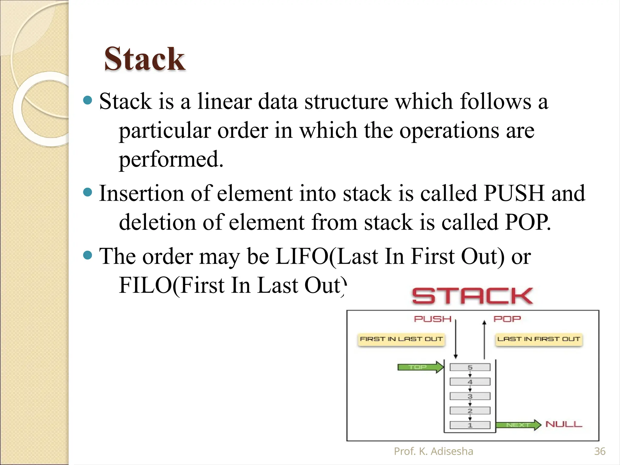
Stack
⚫ Stack isa linear data structure which follows a
particular order in which the operations are
performed.
⚫ Insertion of element into stack is called PUSH and
deletion of element from stack is called POP.
⚫ The order may be LIFO(Last In First Out) or
FILO(First In Last Out).
Prof. K. Adisesha 36
37.
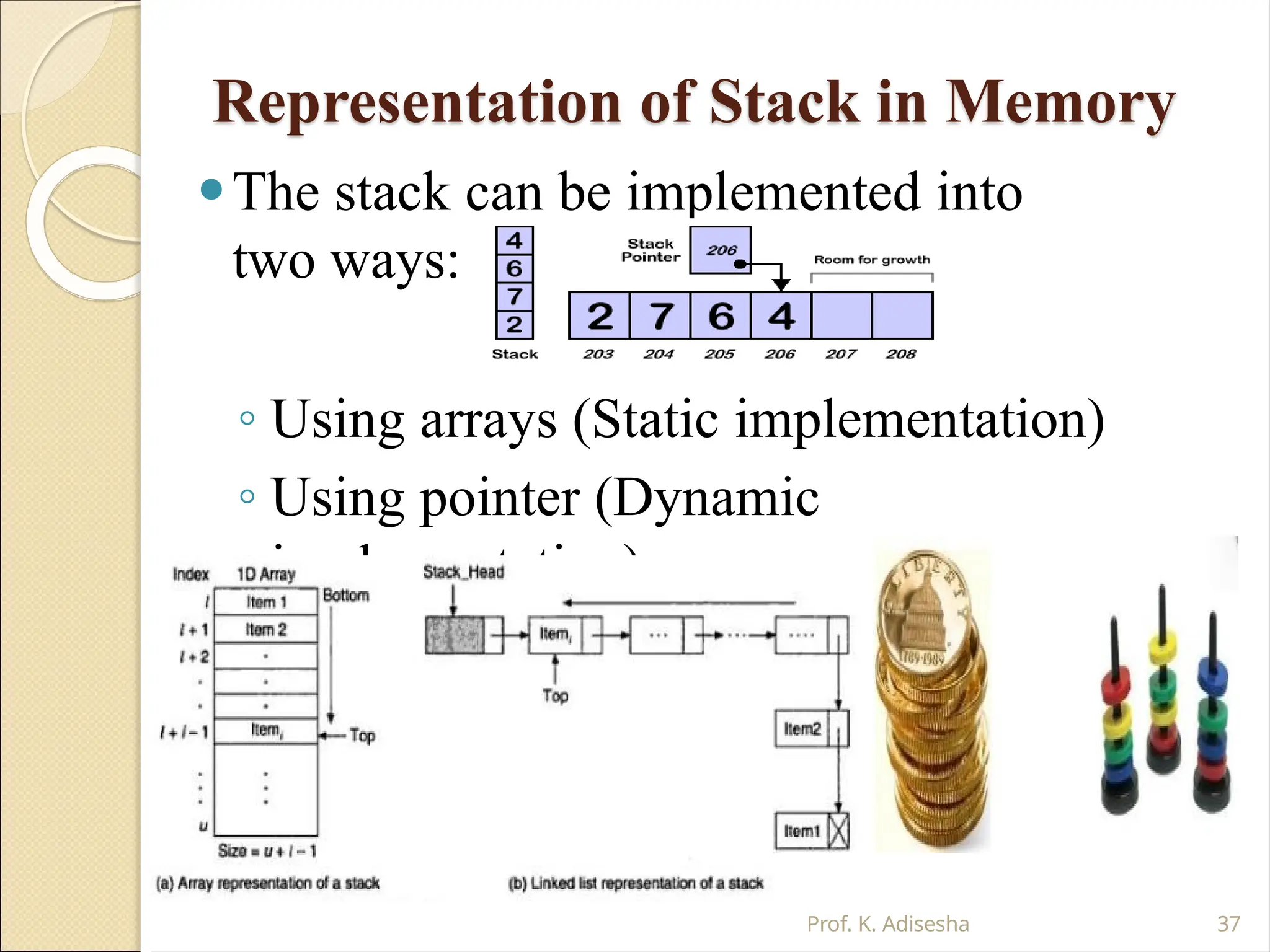
Representation of Stackin Memory
⚫The stack can be implemented into
two ways:
◦ Using arrays (Static implementation)
◦ Using pointer (Dynamic
implementation)
Prof. K. Adisesha 37
38.
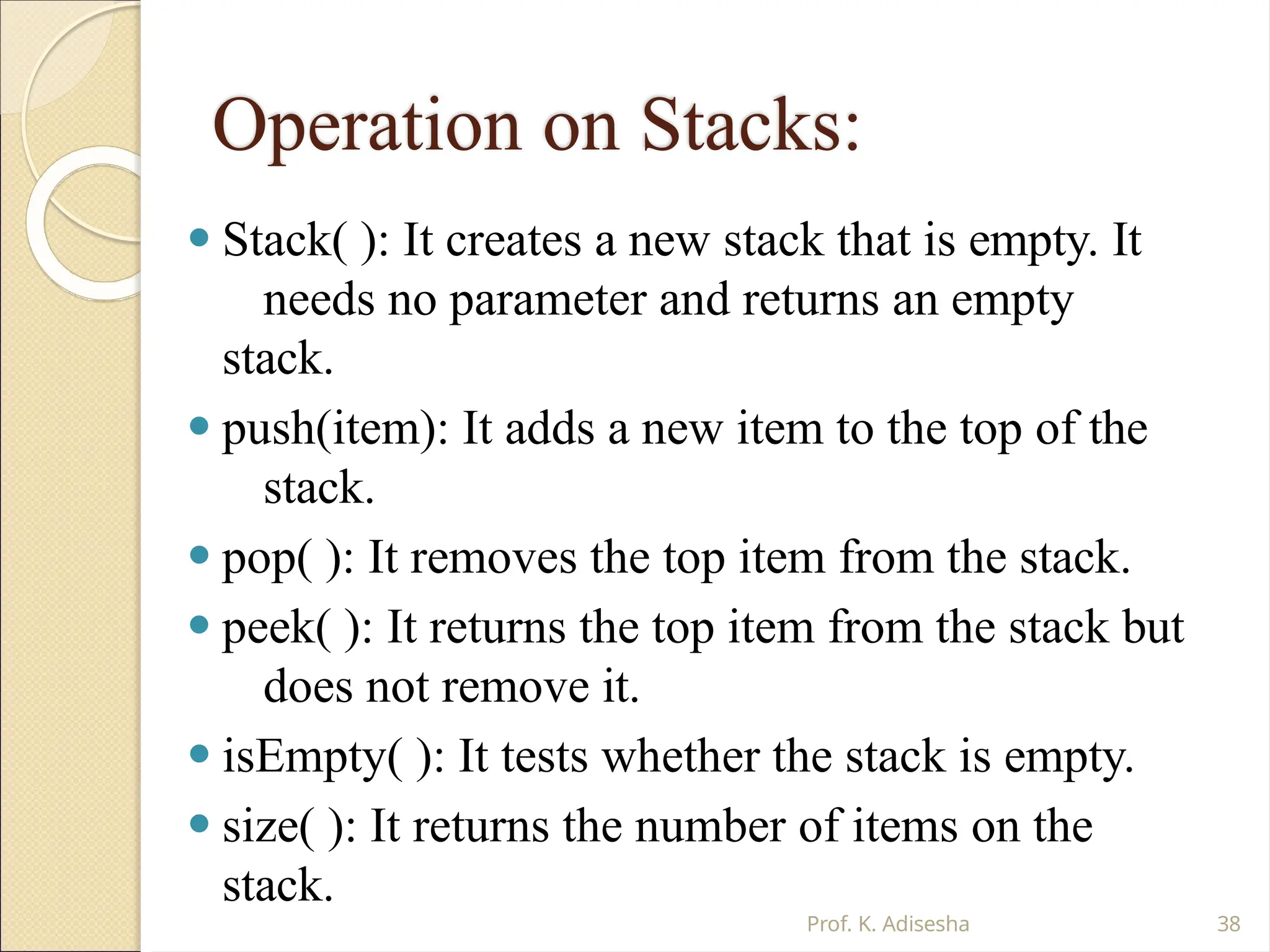
Operation on Stacks:
Prof.K. Adisesha 38
⚫ Stack( ): It creates a new stack that is empty. It
needs no parameter and returns an empty
stack.
⚫ push(item): It adds a new item to the top of the
stack.
⚫ pop( ): It removes the top item from the stack.
⚫ peek( ): It returns the top item from the stack but
does not remove it.
⚫ isEmpty( ): It tests whether the stack is empty.
⚫ size( ): It returns the number of items on the
stack.
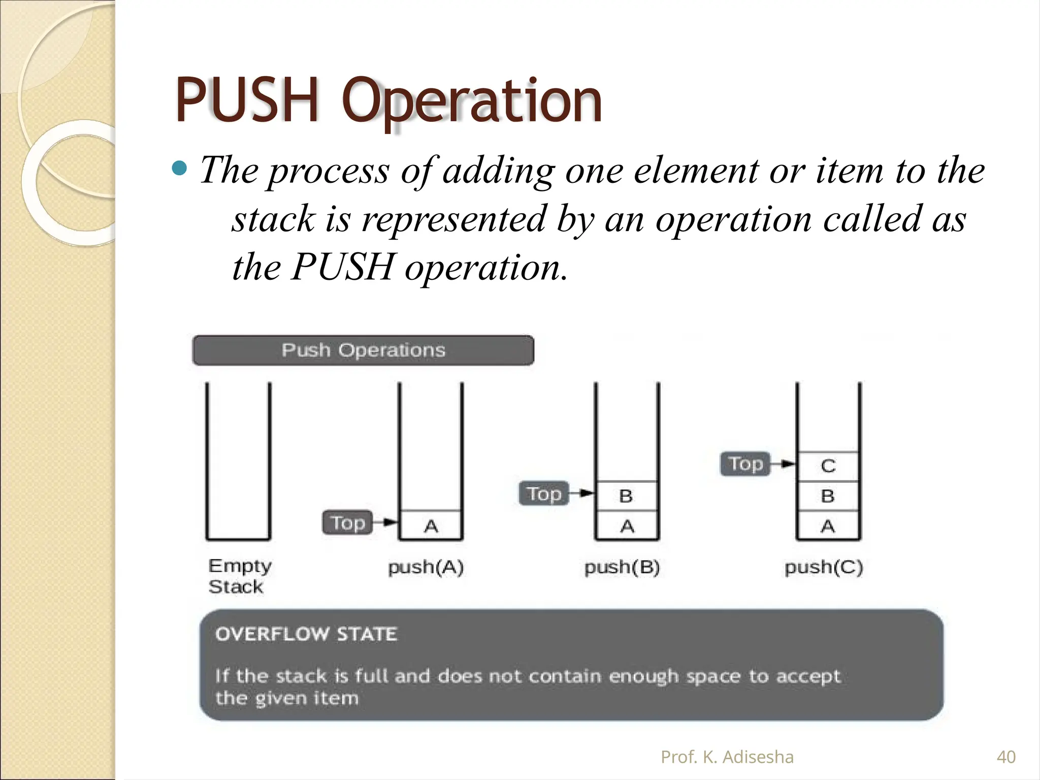
PUSH Operation
⚫ Theprocess of adding one element or item to the
stack is represented by an operation called as
the PUSH operation.
Prof. K. Adisesha 40
41.
PUSH
Operation:
Prof. K. Adisesha41
⚫ The process of adding one element or item to the stack is
represented by an operation called as the PUSH operation.
⚫ The new element is added at the topmost position of the stack.
ALGORITHM:
PUSH (STACK, TOP, SIZE, ITEM)
STACK is the array with N elements. TOP is the pointer to the top of
the element of the array. ITEM to be inserted.
Step 1: if TOP = N then [Check Overflow]
PRINT “ STACK is Full or Overflow”
Exit
[Increment the TOP]
[Insert the ITEM]
[End if]
Step 2: TOP = TOP + 1
Step 3: STACK[TOP] = ITEM
Step 4: Return
42.
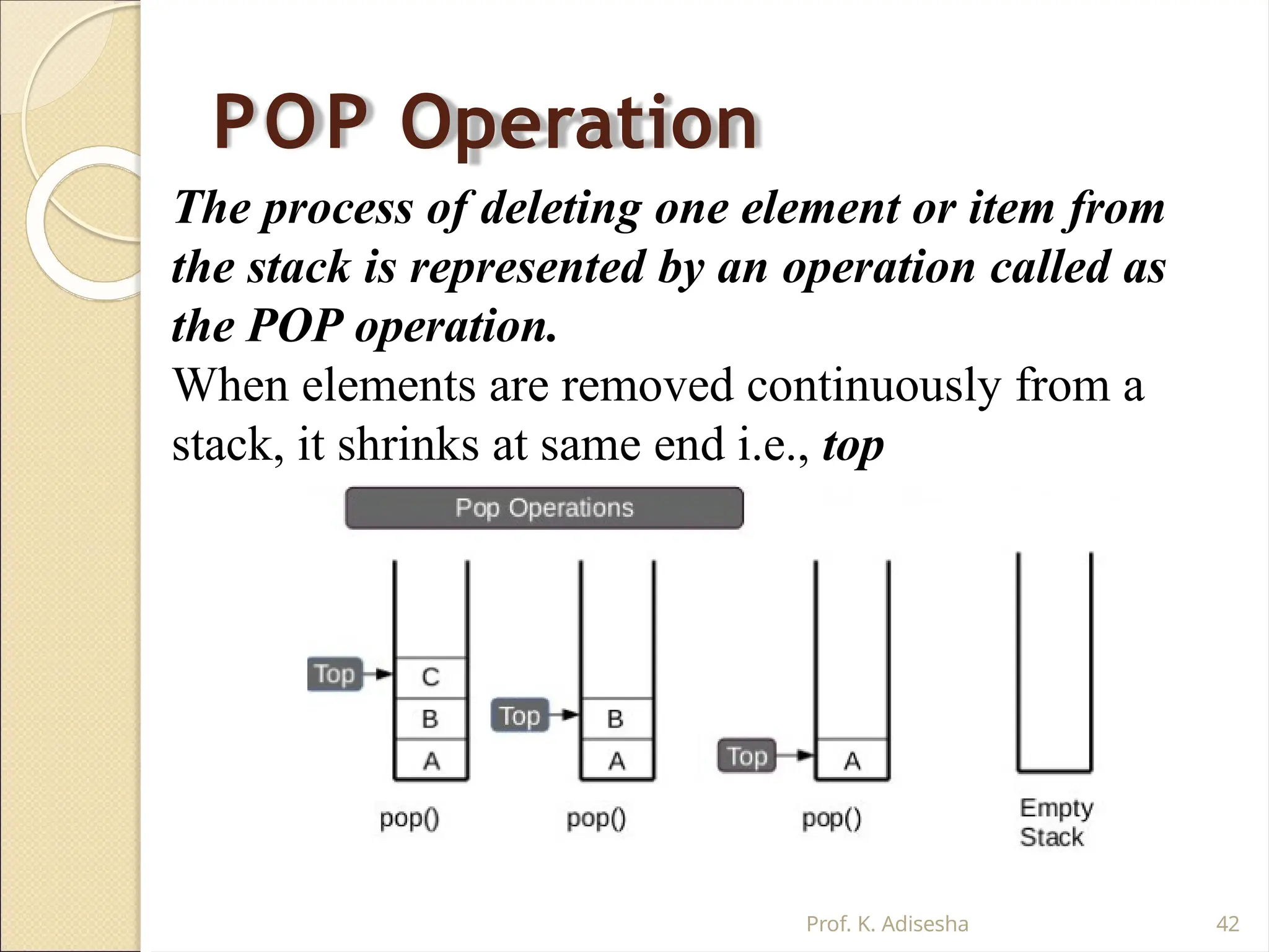
POP Operation
The processof deleting one element or item from
the stack is represented by an operation called as
the POP operation.
When elements are removed continuously from a
stack, it shrinks at same end i.e., top
Prof. K. Adisesha 42
43.
POP Operation
Prof. K.Adisesha 43
The process of deleting one element or item from the
stack is represented by an operation called as the POP
operation.
ALGORITHM: POP (STACK, TOP, ITEM)
STACK is the array with N elements. TOP is the pointer to the top of
the element of the array. ITEM to be inserted.
Step 1: if TOP = 0 then [Check Underflow]
PRINT “ STACK is Empty or
Underflow”
Exit
[End if] [copy the TOP
Element] [Decrement
the TOP]
Step 2: ITEM = STACK[TOP]
Step 3: TOP = TOP - 1
Step 4: Return
44.
PEEK Operation
Prof. K.Adisesha 44
The process of returning the top item from the
stack but does not remove it called as the POP
operation.
ALGORITHM: PEEK (STACK, TOP)
STACK is the array with N elements. TOP is the
pointer to
the top of the element of the array.
Step 1: if TOP = NULL then [Check Underflow]
PRINT “ STACK is Empty or
Underflow”
Exit
[End if]
Step 2: Return (STACK[TOP] [Return the top
45.
Application of Stacks
⚫Runtime memory
management. Prof. K. Adisesha 45
⚫ It is used to reverse a word. You push a given word to
stack – letter by letter and then pop letter from the stack.
⚫ “Undo” mechanism in text editor.
⚫ Backtracking: This is a process when you need to access
the most recent data element in a series of elements.
Once you reach a dead end, you must backtrack.
⚫ Language Processing: Compiler’ syntax check for
matching braces in implemented by using stack.
⚫ Conversion of decimal number to binary.
⚫ To solve tower of Hanoi.
⚫ Conversion of infix expression into prefix and postfix.
⚫ Quick sort
46.
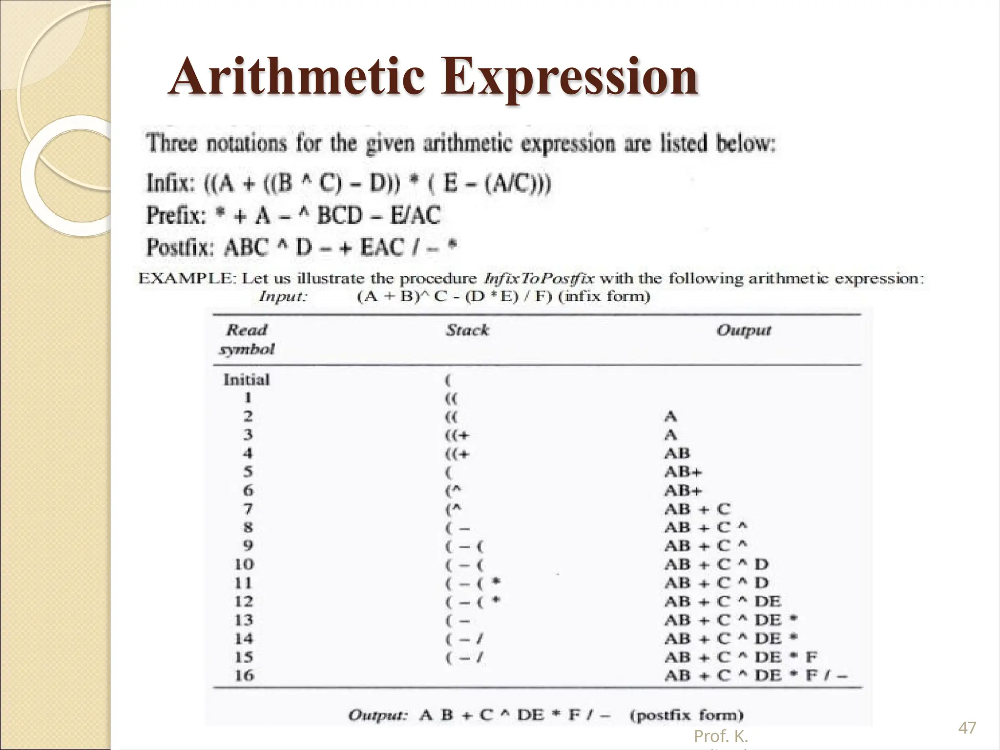
Arithmetic Expression
⚫ Example:+ab
Prof. K. Adisesha 46
⚫ An expression is a combination of operands and
operators that after evaluation results in a single value.
· Operand consists of constants and variables.
· Operators consists of {, +, -, *, /, ), ] etc.
⚫ Expression can be
Infix Expression: If an operator is in between two operands, it is called
infix expression.
⚫ Example: a + b, where a and b are operands and + is an operator.
Postfix Expression: If an operator follows the two operands, it is called
postfix expression.
⚫ Example: ab +
Prefix Expression: an operator precedes the two operands, it is called
prefix expression.
Queue
Prof. K. Adisesha48
⚫ A queue is an ordered collection of items where an
item is inserted at one end called the “rear” and
an existing item is removed at the other end, called
the “front”.
⚫ Queue is also called as FIFO list i.e. First-In First-
Out.
⚫ In the queue only two operations are allowed enqueue
and dequeue.
⚫ Enqueue means to insert an item into back of
the queue.
⚫ Dequeue means removing the front item.The people
standing in a railway reservation row are an
example of queue.
49.
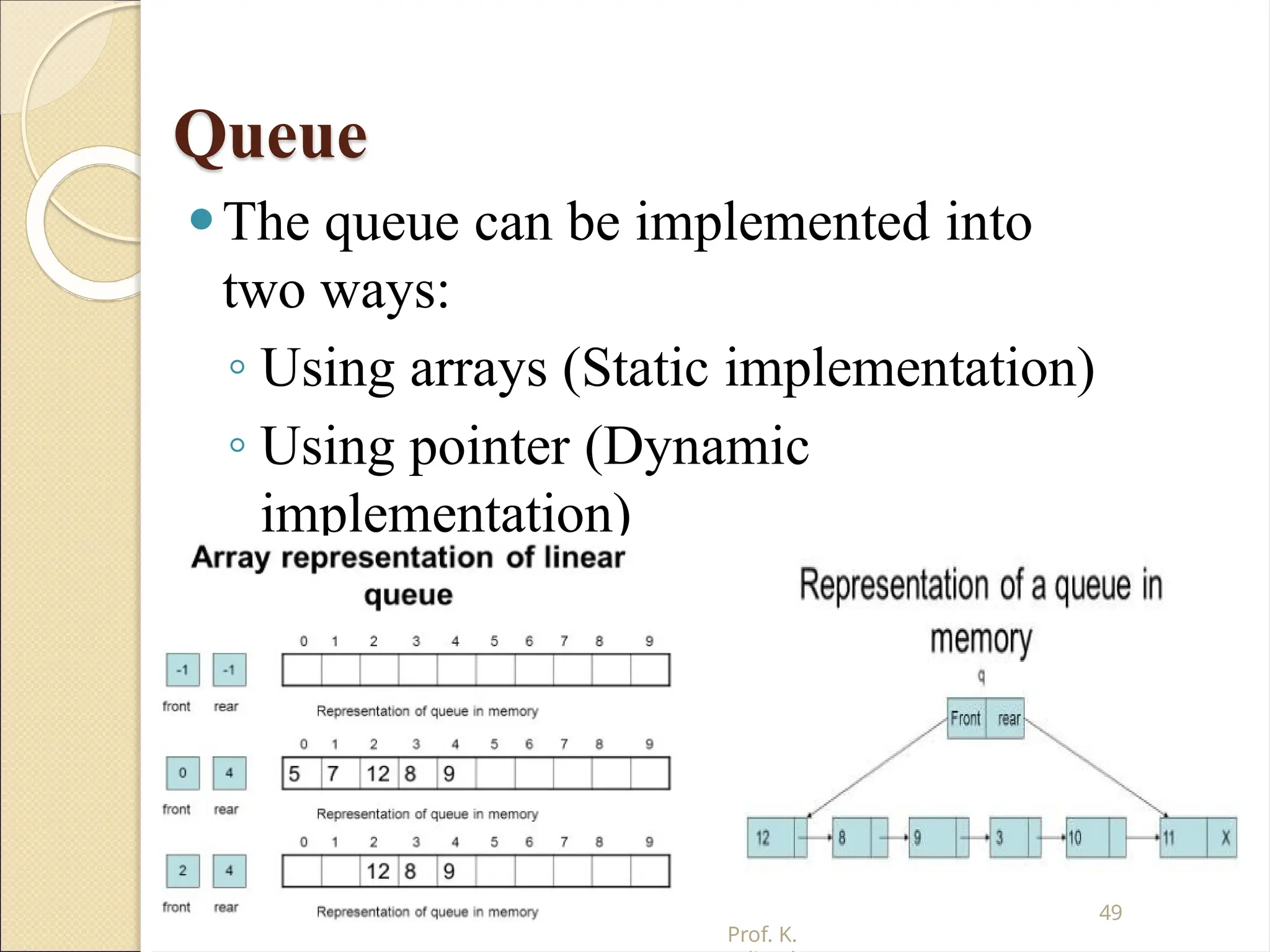
Queue
⚫The queue canbe implemented into
two ways:
◦ Using arrays (Static implementation)
◦ Using pointer (Dynamic
implementation)
49
Prof. K.
50.
Types of Queues
Prof.K. Adisesha 50
⚫Queue can be of four types:
o Simple Queue
o Circular Queue
o Priority Queue
o De-queue ( Double Ended
Queue)
51.
Simple Queue
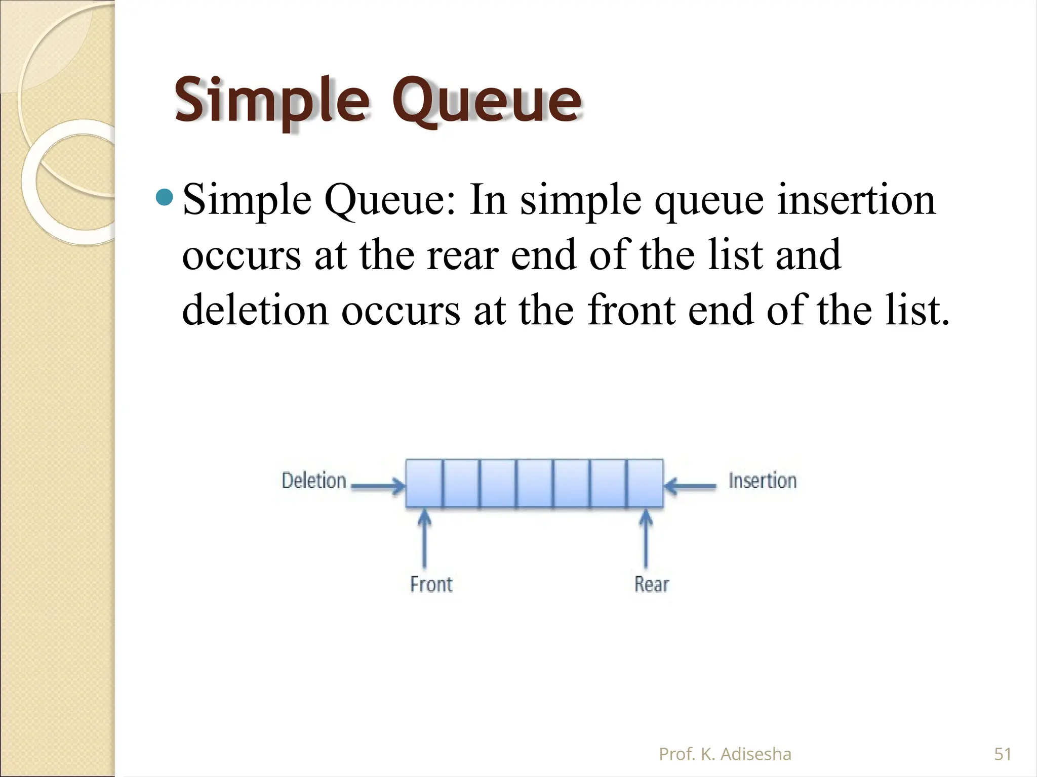
⚫Simple Queue:In simple queue insertion
occurs at the rear end of the list and
deletion occurs at the front end of the list.
Prof. K. Adisesha 51
52.
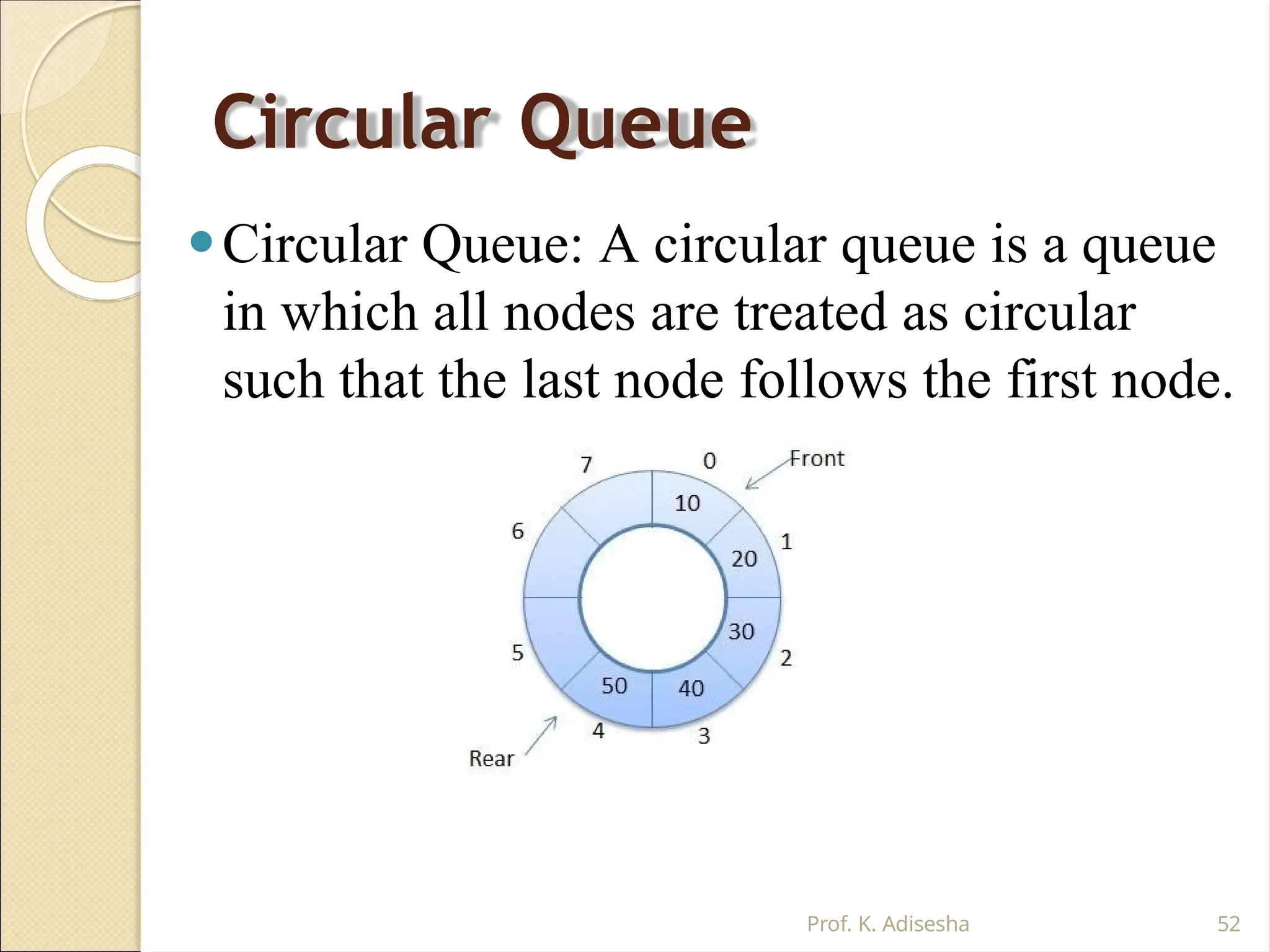
Circular Queue
⚫Circular Queue:A circular queue is a queue
in which all nodes are treated as circular
such that the last node follows the first node.
Prof. K. Adisesha 52
53.
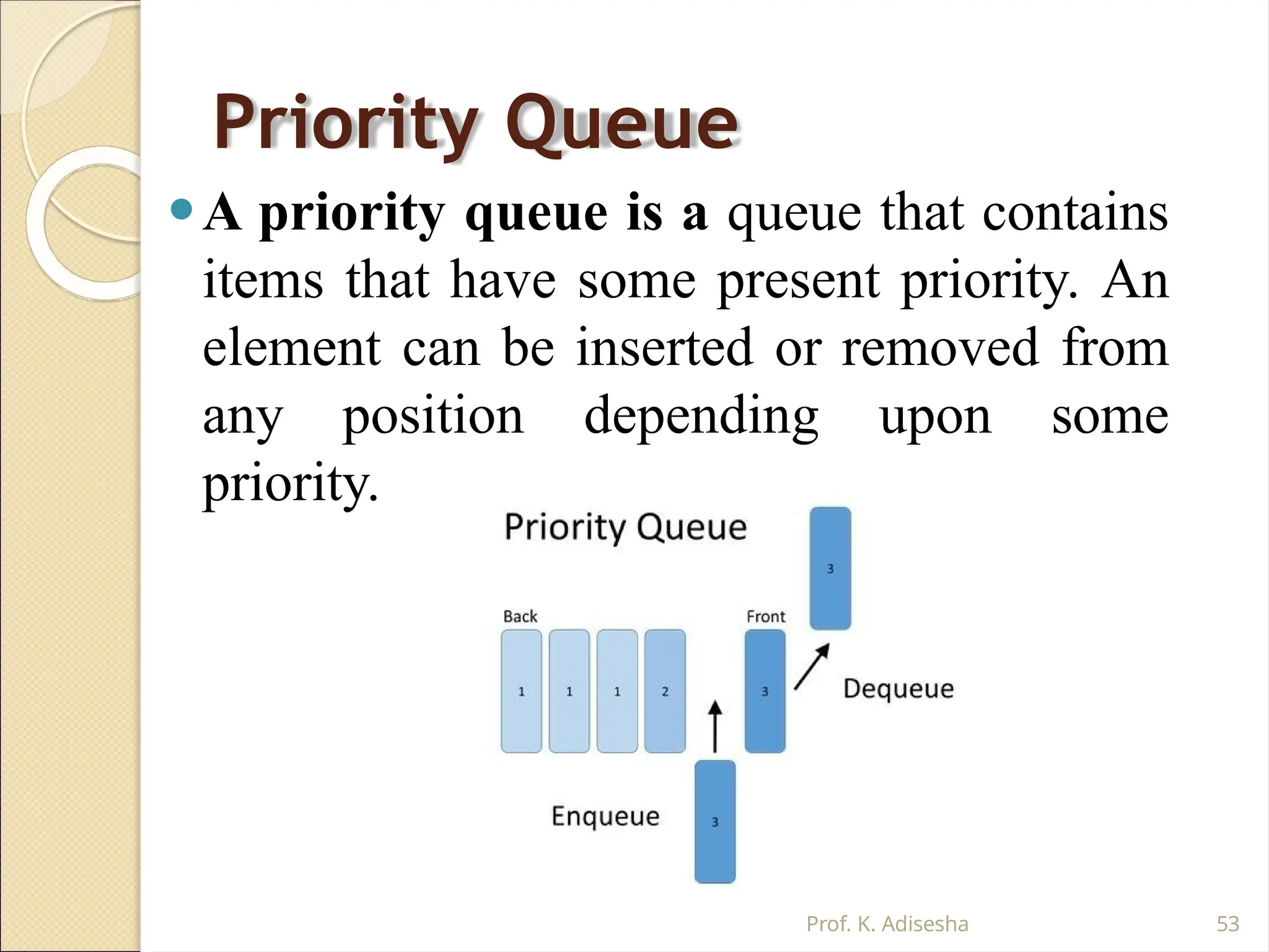
Priority Queue
⚫A priorityqueue is a queue that contains
items that have some present priority. An
element can be inserted or removed from
any position depending upon some
priority.
Prof. K. Adisesha 53
54.
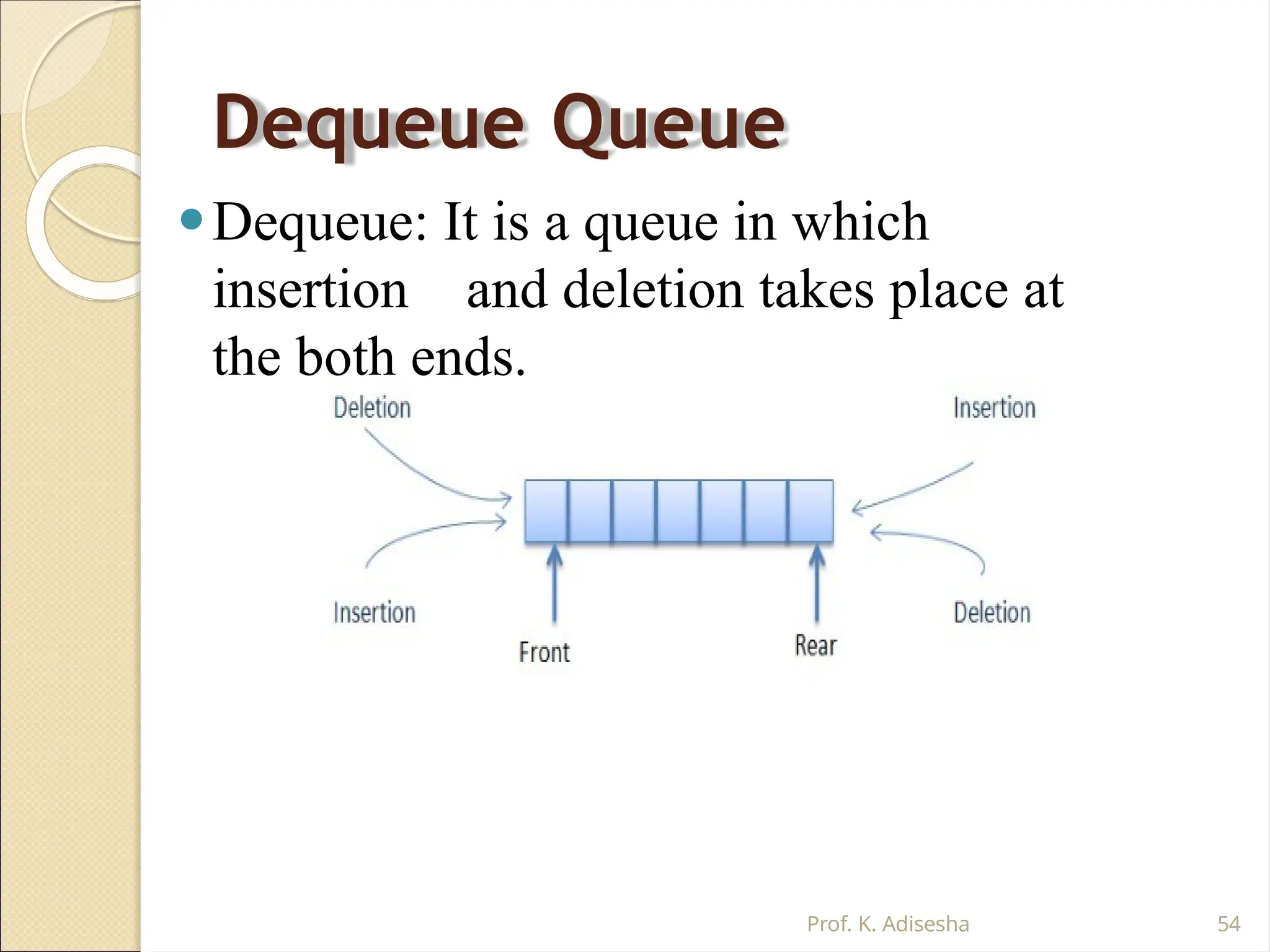
Dequeue Queue
⚫Dequeue: Itis a queue in which
insertion and deletion takes place at
the both ends.
Prof. K. Adisesha 54
55.
Operation on Queues
Prof.K. Adisesha 55
⚫Queue( ): It creates a new queue that is
empty.
⚫enqueue(item): It adds a new item to the rear
of the queue.
⚫dequeue( ): It removes the front item from
the queue.
⚫isEmpty( ): It tests to see whether the queue
is empty.
⚫size( ): It returns the number of items in the
queue.
56.
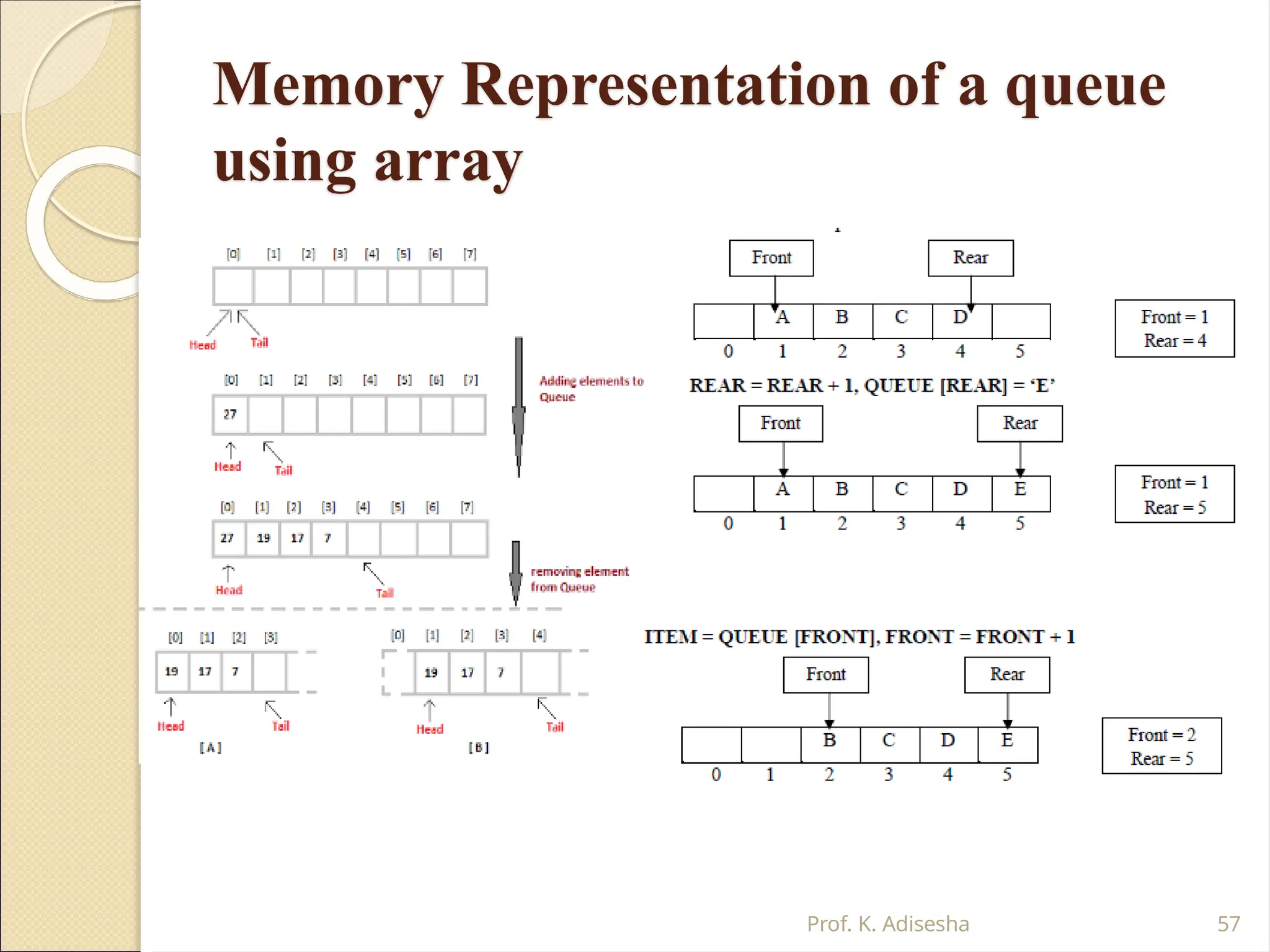
Memory Representation ofa queue
using array
Prof. K. Adisesha 56
⚫ Queue is represented in memory using linear
array.
⚫ Let QUEUE is a array, two pointer variables
called FRONT and REAR are maintained.
⚫ The pointer variable FRONT contains the location of
the element to be removed or deleted.
⚫ The pointer variable REAR contains location of the last
element inserted.
⚫ The condition FRONT = NULL indicates that queue is
empty.
⚫ The condition REAR = N-1 indicates that queue is full.
Queue Insertion
Operation (ENQUEUE):
⚫ALGORITHM: ENQUEUE (QUEUE, REAR, FRONT, ITEM)
QUEUE is the array with N elements. FRONT is the pointer that contains
the location of the element to be deleted and REAR contains the location of
the inserted element. ITEM is the element to be inserted.
Step 1: if REAR = N-1 then [Check Overflow]
PRINT “QUEUE is Full or Overflow”
Exit [End if]
Step 2: if FRONT = NULL then [Check Whether Queue is
empty] FRONT = -1
REAR = -1
else
REAR = REAR + 1 [Increment REAR Pointer]
Step 3: QUEUE[REAR] = ITEM [Copy ITEM to REAR position]
Step 4: Return
Prof. K. Adisesha 58
59.
Queue Deletion Operation
(DEQUEUE)
ALGORITHM:DEQUEUE (QUEUE, REAR, FRONT, ITEM)
QUEUE is the array with N elements. FRONT is the pointer that contains
the location of the element to be deleted and REAR contains the location of
the inserted element. ITEM is the element to be inserted.
Step 1: if FRONT = NULL then [Check Whether Queue is
empty] PRINT “QUEUE is Empty or Underflow”
Exit [End
if]
Step 2:
ITEM =
QUEUE[F
RONT]
Step 3: if FRONT = REAR then [if QUEUE has only one
element] FRONT = NULL
REAR = NULL
else
Step 4: Return
Prof. K. Adisesha 59
60.
Application of Queue
Prof.K. Adisesha 60
⚫Simulation
⚫Various features of Operating system
⚫Multi-programming platform systems.
⚫Different types of scheduling
algorithms
⚫Round robin technique algorithms
⚫Printer server routines
⚫Various application software’s is also
based on queue data structure.
61.
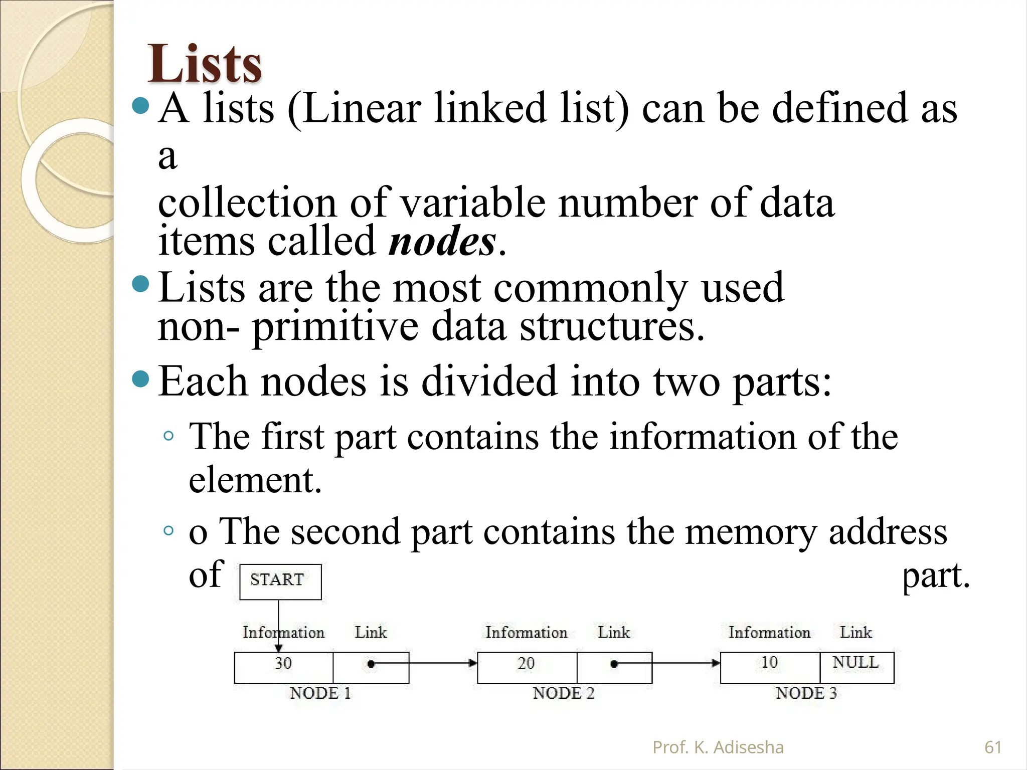
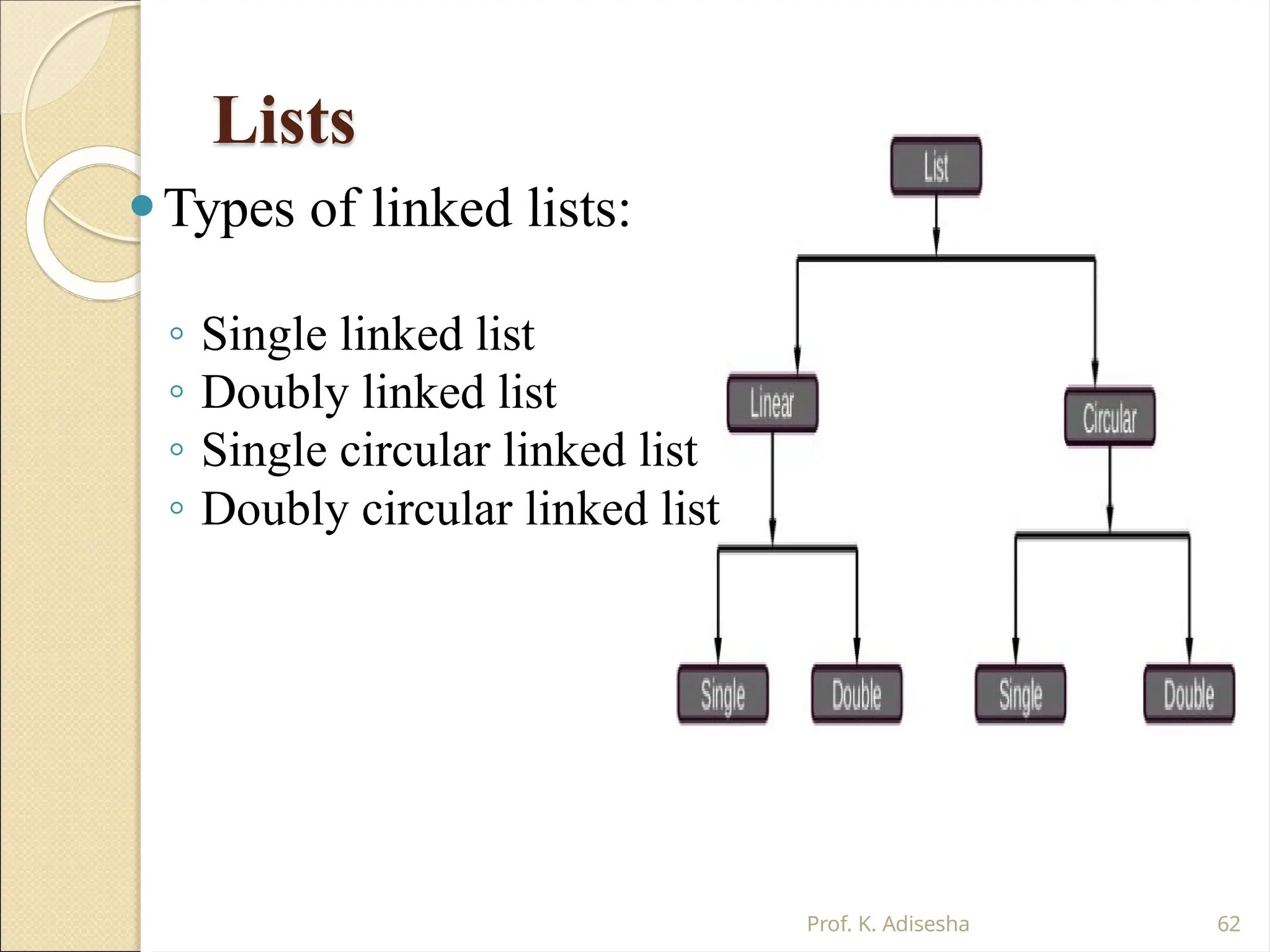
Lists
⚫A lists (Linearlinked list) can be defined as
a
collection of variable number of data
items called nodes.
⚫Lists are the most commonly used
non- primitive data structures.
⚫Each nodes is divided into two parts:
◦ The first part contains the information of the
element.
◦ o The second part contains the memory address
of the next node in the list. Also called Link part.
Prof. K. Adisesha 61
62.
Lists
Prof. K. Adisesha62
⚫Types of linked lists:
◦ Single linked list
◦ Doubly linked list
◦ Single circular linked list
◦ Doubly circular linked list
63.
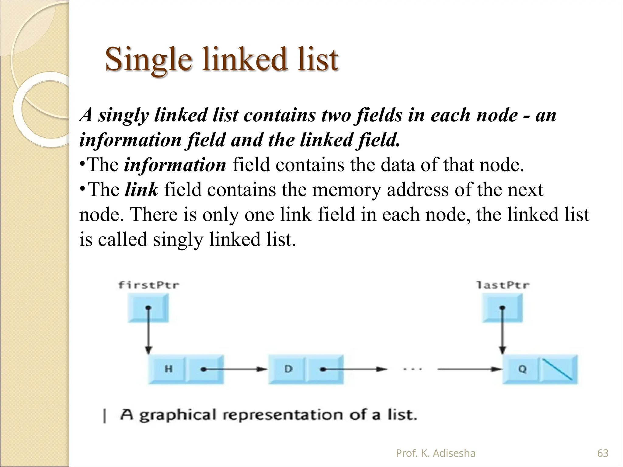
Single linked list
Asingly linked list contains two fields in each node - an
information field and the linked field.
•The information field contains the data of that node.
•The link field contains the memory address of the next
node. There is only one link field in each node, the linked list
is called singly linked list.
Prof. K. Adisesha 63
64.
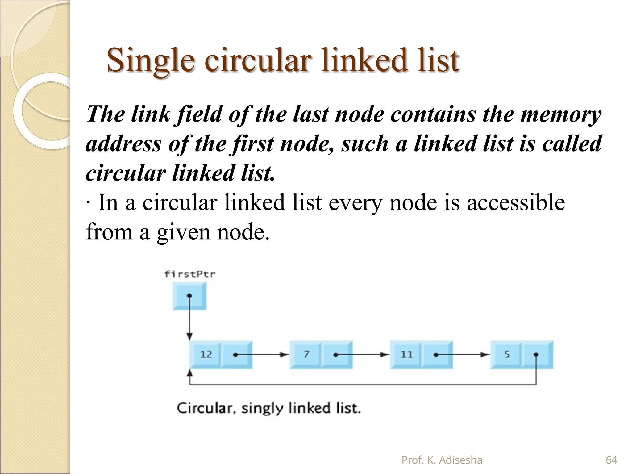
Single circular linkedlist
The link field of the last node contains the memory
address of the first node, such a linked list is called
circular linked list.
· In a circular linked list every node is accessible
from a given node.
Prof. K. Adisesha 64
65.
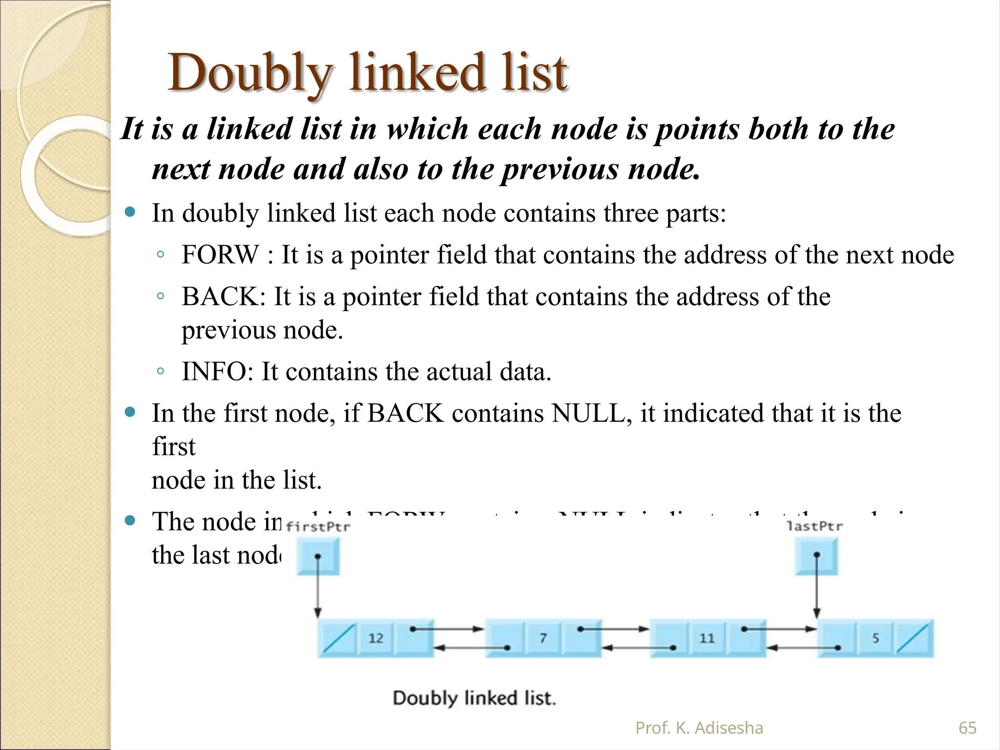
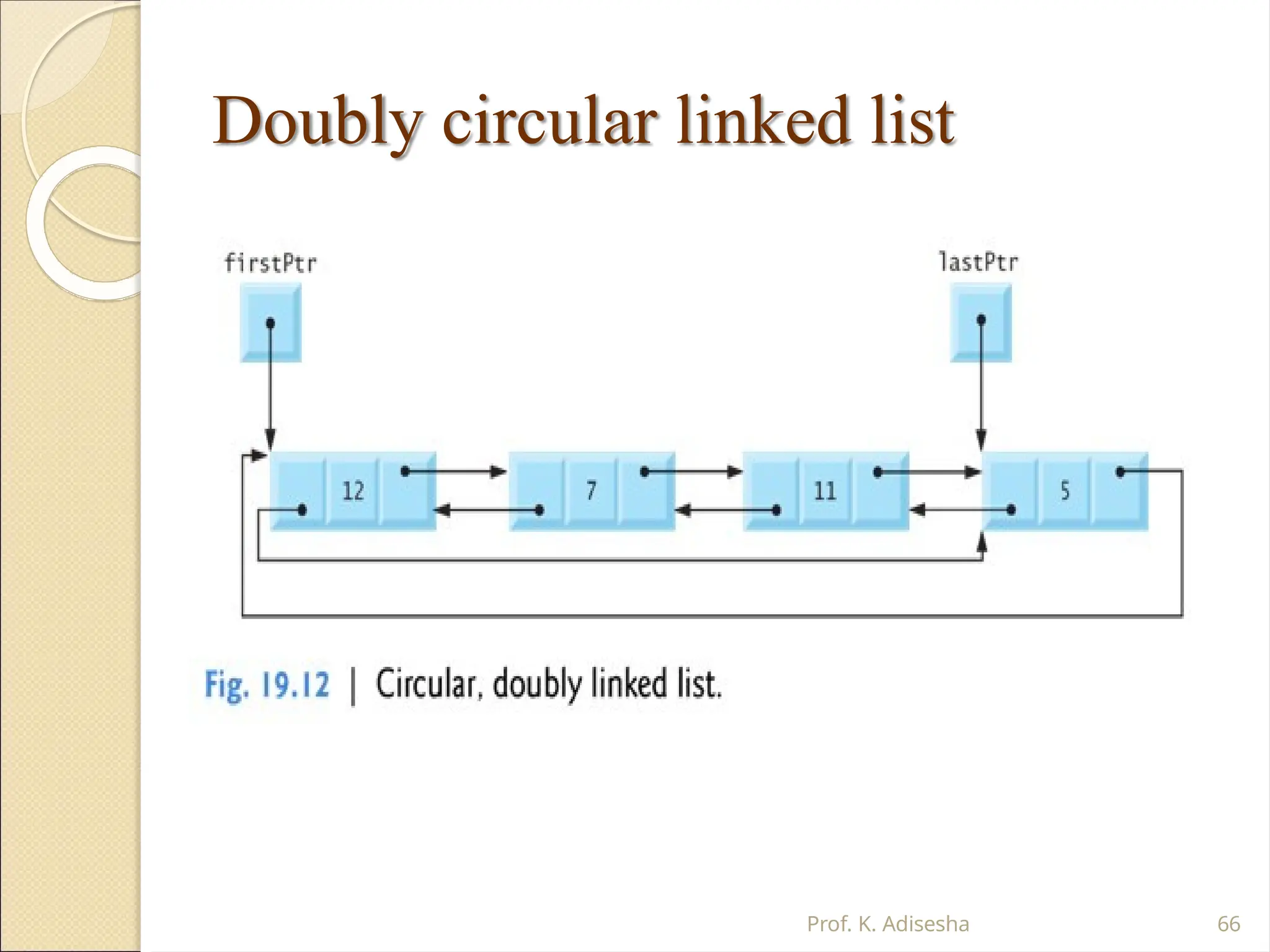
Doubly linked list
Itis a linked list in which each node is points both to the
next node and also to the previous node.
⚫ In doubly linked list each node contains three parts:
◦ FORW : It is a pointer field that contains the address of the next node
◦ BACK: It is a pointer field that contains the address of the
previous node.
◦ INFO: It contains the actual data.
⚫ In the first node, if BACK contains NULL, it indicated that it is the
first
node in the list.
⚫ The node in which FORW contains, NULL indicates that the node is
the last node.
Prof. K. Adisesha 65
Operation on LinkedList
Prof. K. Adisesha 67
⚫The operation that are performed
on linked lists are:
◦ Creating a linked list
◦ Traversing a linked list
◦ Inserting an item into a linked list.
◦ Deleting an item from the linked list.
◦ Searching an item in the linked list
◦ Merging two or more linked lists.
68.
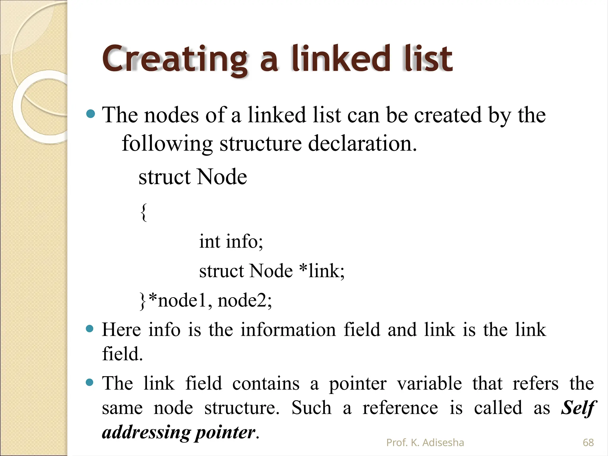
Creating a linkedlist
Prof. K. Adisesha 68
⚫ The nodes of a linked list can be created by the
following structure declaration.
struct Node
{
int info;
struct Node *link;
}*node1, node2;
⚫ Here info is the information field and link is the link
field.
⚫ The link field contains a pointer variable that refers the
same node structure. Such a reference is called as Self
addressing pointer.
69.
Operator new and
delete
Prof.K. Adisesha 69
⚫Operators new allocate memory
space.
◦ Operators new [ ] allocates memory
space for array.
⚫Operators delete deallocate
memory space.
◦ Operators delete [ ] deallocate
memory space for array.
70.
Traversing a linkedlist:
Prof. K. Adisesha 70
⚫ Traversing is the process of accessing each node of
the linked list exactly once to perform some operation.
⚫ ALGORITHM: TRAVERS (START, P) START
contains
the address of the first node. Another pointer p is
temporarily used to visit all the nodes from the beginning
to the end of the linked list.
Step 1: P = START
Step 2: while P != NULL
Step 3:
Step 4:
PROCESS data (P)
P = link(P)
[Fetch the data]
[Advance P to next
node]
Step 5: End of while
Step 6: Return
71.
Inserting a nodeinto the
linked list
Prof. K. Adisesha 71
⚫Inserting a node at the beginning of
the linked list
⚫Inserting a node at the given
position.
⚫Inserting a node at the end of the
linked list.
72.
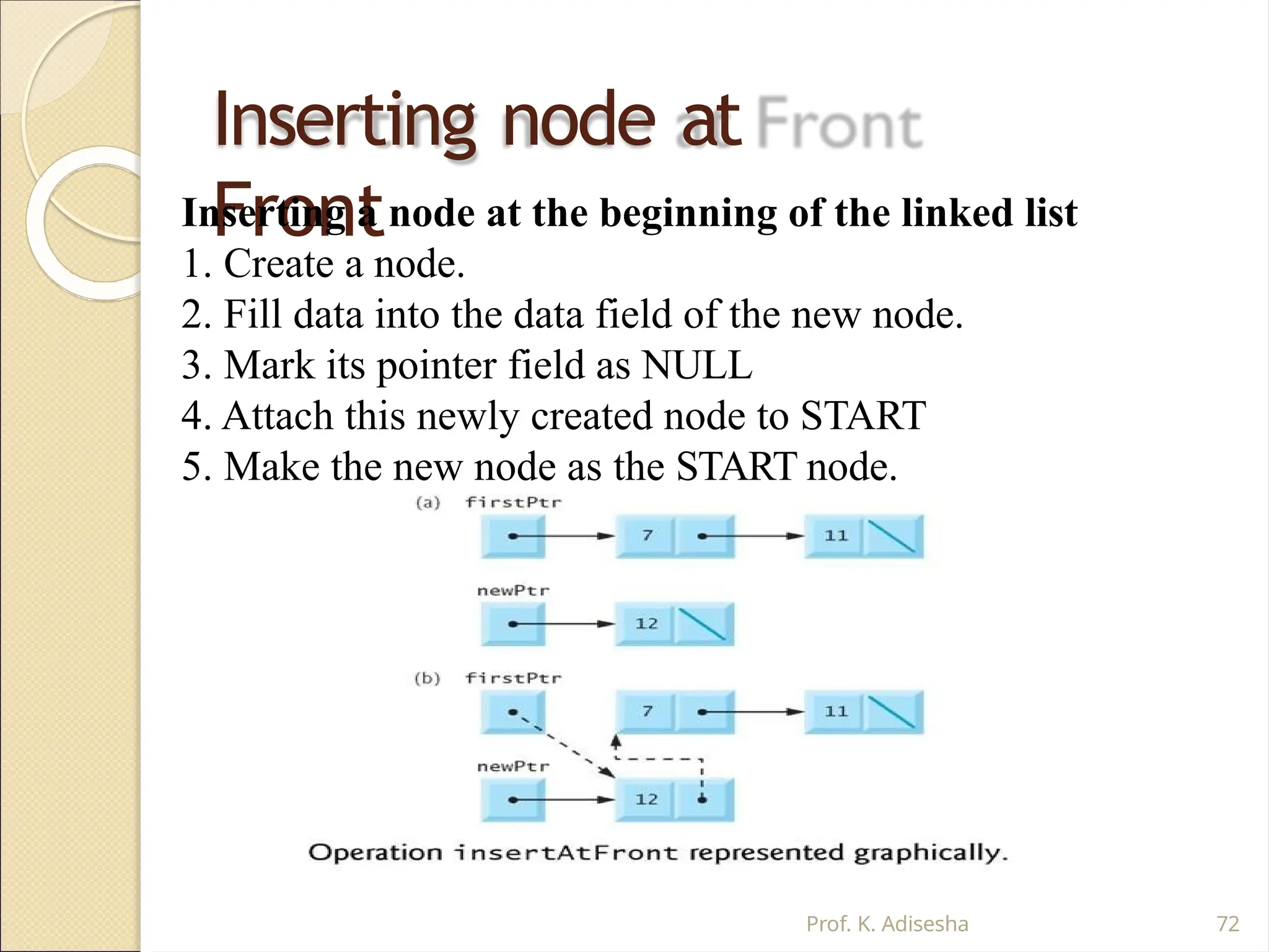
Inserting node at
Front
Insertinga node at the beginning of the linked list
1. Create a node.
2. Fill data into the data field of the new node.
3. Mark its pointer field as NULL
4. Attach this newly created node to START
5. Make the new node as the START node.
Prof. K. Adisesha 72
73.
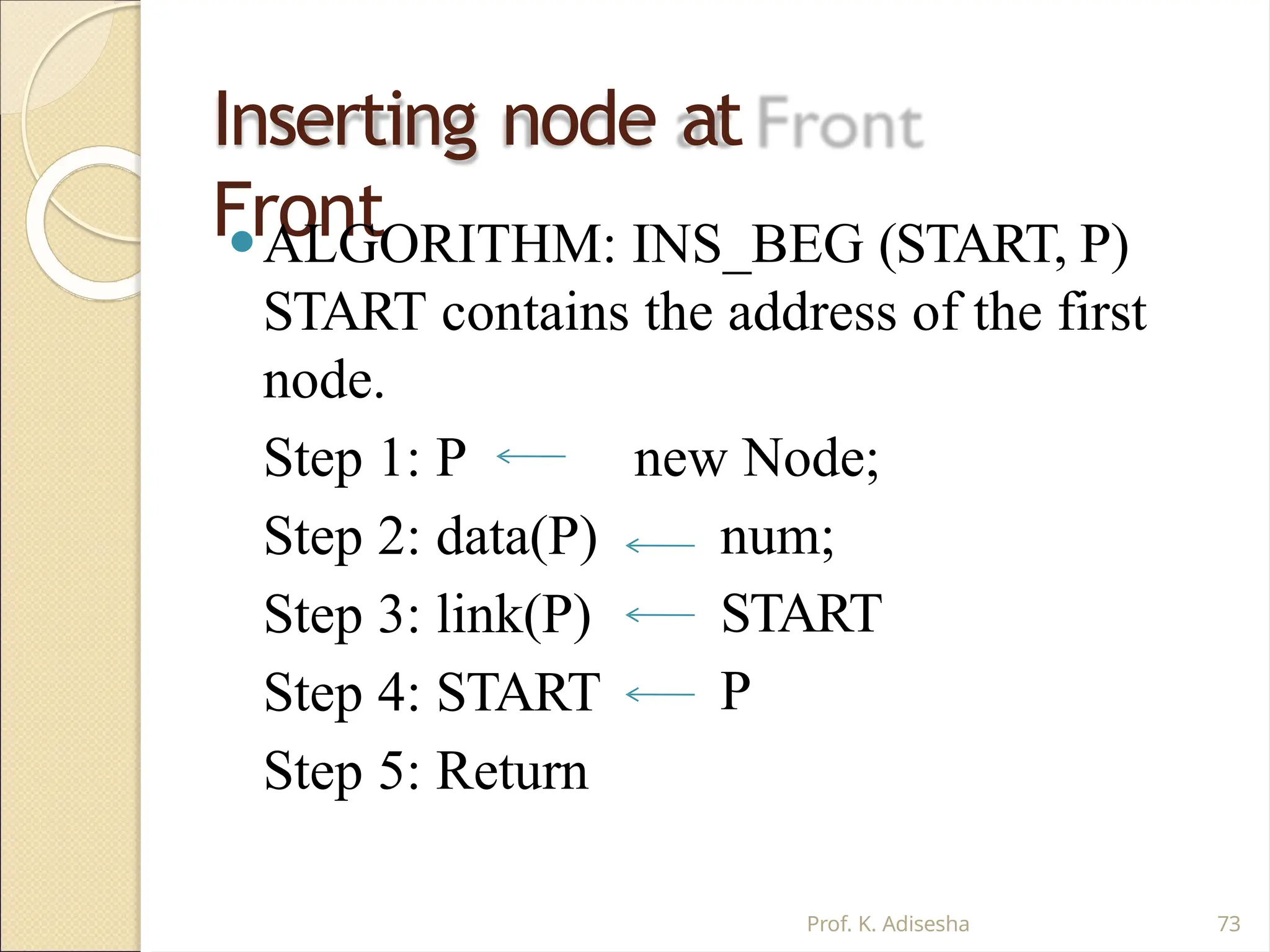
Inserting node at
Front
⚫ALGORITHM:INS_BEG (START, P)
START contains the address of the first
node.
Step 1: P new Node;
num;
START
P
Step 2: data(P)
Step 3: link(P)
Step 4: START
Step 5: Return
Prof. K. Adisesha 73
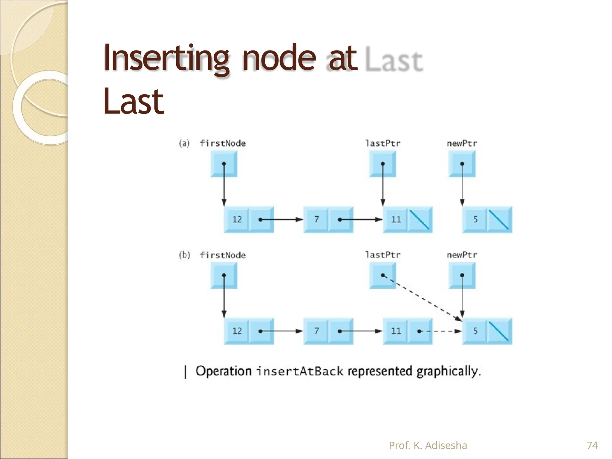
Inserting node at
Last
⚫ALGORITHM: INS_END (START, P) START contains
the address of the first node.
Step 1: START
Step 2: P START [identify the last node]
while P!= null
P
next (P) End
while
Step 3: N new
Node;
Step 4: data(N)
item; Step 5: link(N)
null Step 6: link(P) N
Step 7: Return Prof. K. 75
76.
Inserting node ata given Position
count+1
next (P)
Count 0
Step 3: while P!= null
count
P
E
n
d
w
h
i
l
Call function INS_BEG( )
else if (POS=Count +1)
Call function
INS_END( )
For(i=1; i<=pos; i++)
P
next(P);
end for new node
item;
link(P)
N
[create] N
data(N)
link(N)
link(P)
else
PRINT “Invalid position”
Step 5:
Return
ALGORITHM: INS_POS (START, P) START contains the
address of the first node.
Step 1: START else if
(POS<=Count) Step 2: P START [Initialize
node] P Start
Prof. K. Adisesha 76
77.
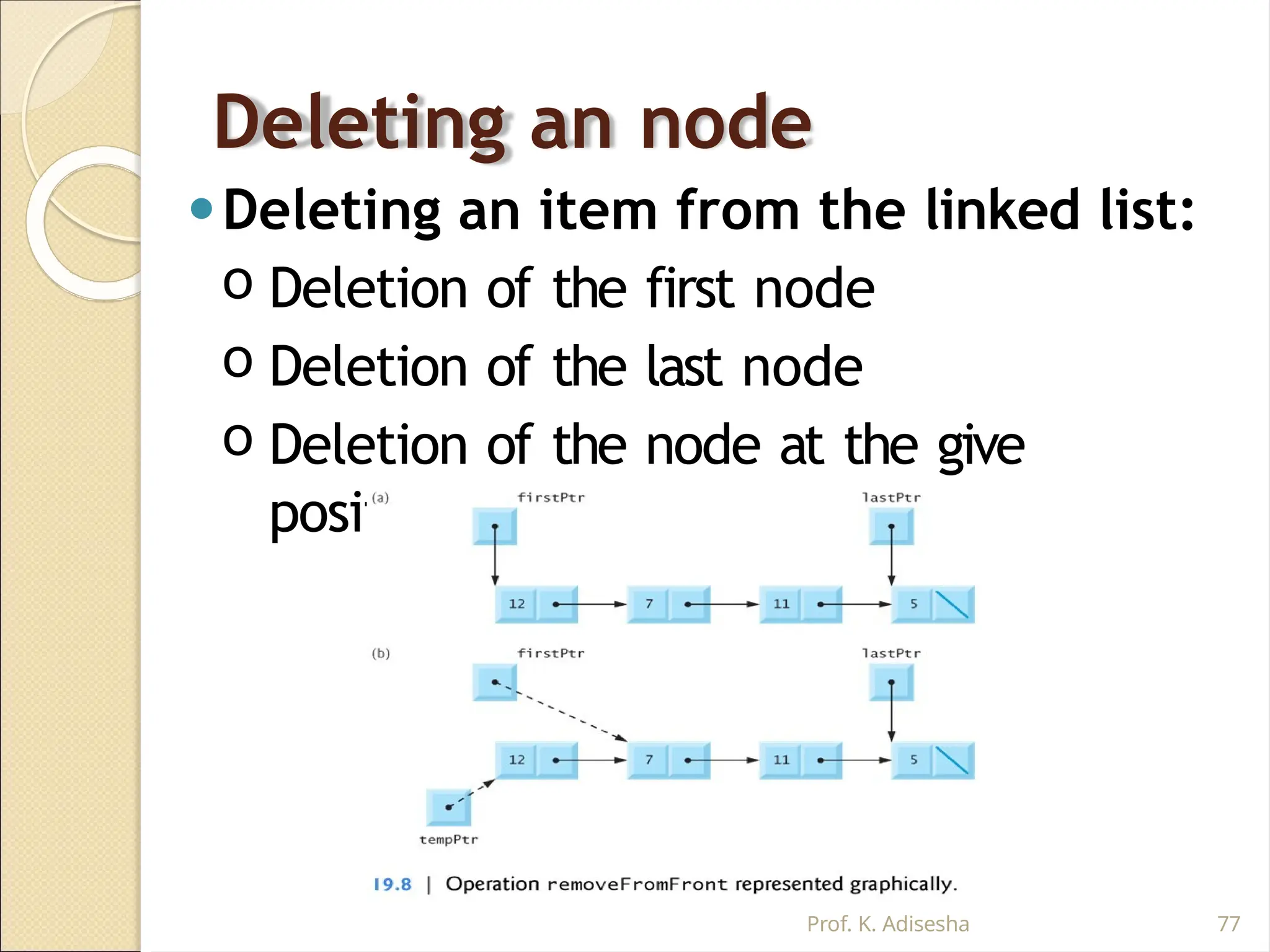
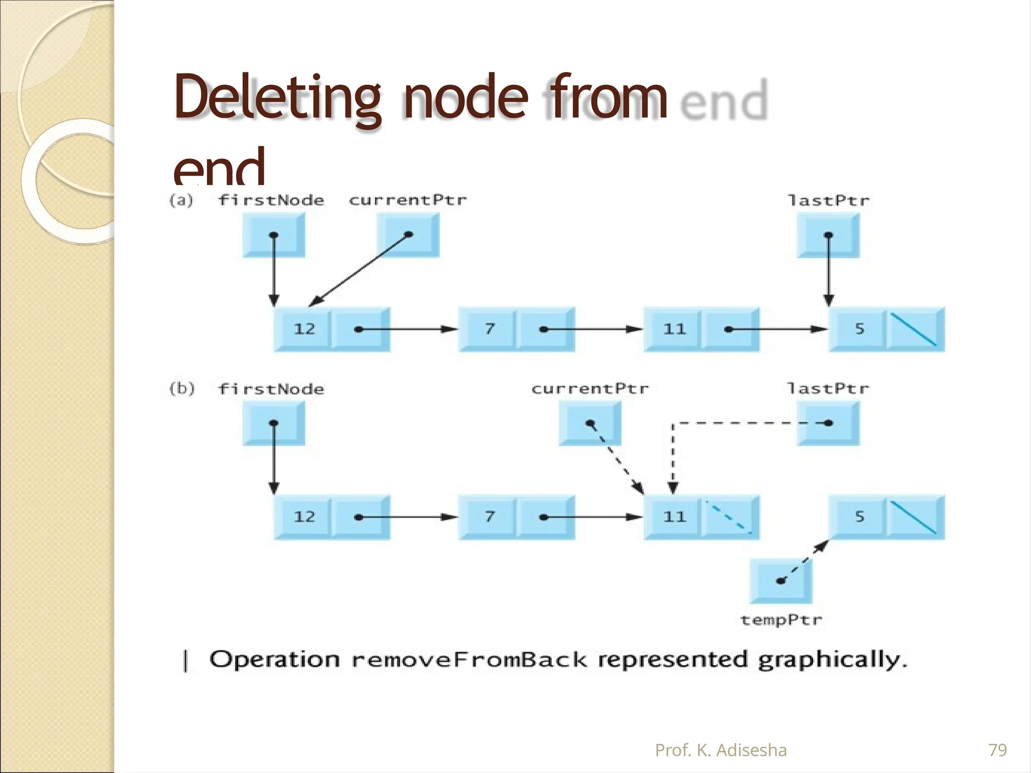
Deleting an node
⚫Deletingan item from the linked list:
o Deletion of the first node
o Deletion of the last node
o Deletion of the node at the give
position
Prof. K. Adisesha 77
78.
Deleting node from
end
ALGORITHM:DEL_END (P1, P2, START) This used two
pointers P1 and P2. Pointer P2 is used to traverse the linked
list and pointer P1 keeps the location of the previous node of
P2.
Step 1: START
Step 2: P2 START;
Step 3: while ( link(P2) ! =
NULL) P1 P2
P2
link(P2) While
end
Step 4: PRINT data(p2)
NULL
Step 5: link(P1)
Free(P2)
Step 6: STOP
Prof. K. Adisesha 78
Non-Linear Data structures
Prof.K. Adisesha 80
⚫ A Non-Linear Data structures is a data structure
in which data item is connected to several
other data items.
⚫ The data items in non-linear data structure
represent hierarchical relationship.
⚫ Each data item is called node.
⚫ The different non-linear data structures
are
◦ Trees
◦ Graphs.
81.
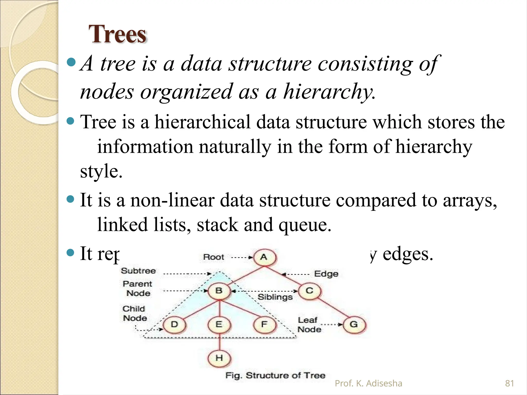
Trees
⚫A tree isa data structure consisting of
nodes organized as a hierarchy.
⚫ Tree is a hierarchical data structure which stores the
information naturally in the form of hierarchy
style.
⚫ It is a non-linear data structure compared to arrays,
linked lists, stack and queue.
⚫ It represents the nodes connected by edges.
Prof. K. Adisesha 81
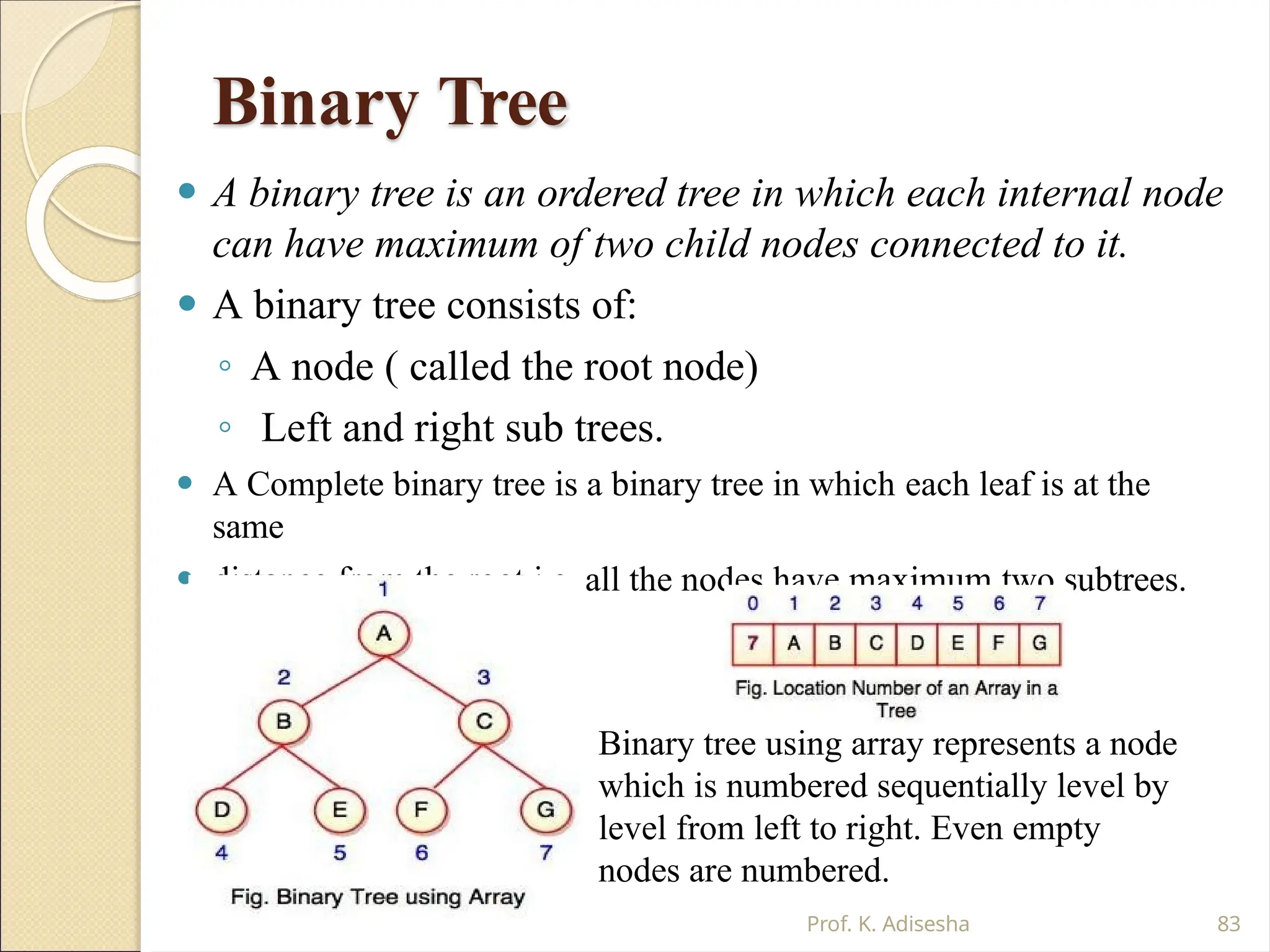
Binary Tree
⚫ Abinary tree is an ordered tree in which each internal node
can have maximum of two child nodes connected to it.
⚫ A binary tree consists of:
◦ A node ( called the root node)
◦ Left and right sub trees.
⚫ A Complete binary tree is a binary tree in which each leaf is at the
same
⚫ distance from the root i.e. all the nodes have maximum two subtrees.
Binary tree using array represents a node
which is numbered sequentially level by
level from left to right. Even empty
nodes are numbered.
Prof. K. Adisesha 83
84.
Graph
Prof. K. Adisesha84
⚫ Graph is a mathematical non-linear data
structure capable of representing many kind of
physical structures.
⚫ A graph is a set of vertices and edges
which connect them.
⚫ A graph is a collection of nodes called vertices
and the connection between them called
edges.
⚫ Definition: A graph G(V,E) is a set of vertices V
and a set of edges E.
Graph
Prof. K. Adisesha86
⚫An edge connects a pair of vertices and
many have weight such as length, cost
and another measuring instrument for
according the graph.
⚫Vertices on the graph are shown as point
or circles and edges are drawn as arcs
or line segment.
87.
Graph
Prof. K. Adisesha87
⚫Types of Graphs:
◦ Directed graph
◦ Undirected
graph
◦ Simple graph
◦ Weighted
graph
◦ Connected
graph
◦ Non-
![One dimensional array:
Prof. K. Adisesha 13
⚫ An array with only one row or column is called one-dimensional
array.
⚫ It is finite collection of n number of elements of same type such
that:
◦ can be referred by indexing.
◦ The syntax Elements are stored in continuous locations.
◦ Elements x to define one-dimensional array is:
⚫ Syntax: Datatype Array_Name [Size];
⚫ Where,
Datatype : Type of value it can store (Example: int, char, float)
Array_Name: To identify the array.
⚫ Size : The maximum number of elements that the array can hold.](https://image.slidesharecdn.com/datastructure-250918053724-5a9ac96c/75/datastructure-and-alogrithm-and-operation-pptx-13-2048.jpg)
![Arrays
Prof. K. Adisesha 14
⚫Simply, declaration of array is as follows:
int arr[10]
⚫Where int specifies the data type or type
of elements arrays stores.
⚫“arr” is the name of array & the number
specified inside the square brackets is the
number of elements an array can store, this
is also called sized or length of array.](https://image.slidesharecdn.com/datastructure-250918053724-5a9ac96c/75/datastructure-and-alogrithm-and-operation-pptx-14-2048.jpg)
![Arrays
Prof. K. Adisesha 16
◦ The elements of array will always be stored in the
consecutive (continues) memory location.
◦ The number of elements that can be stored in an
array, that is the size of array or its length is given
by the following equation:
(Upperbound-lowerbound)+1
◦ For the above array it would be (9-0)+1=10,where 0
is the lower bound of array and 9 is the upper bound
of array.
◦ Array can always be read or written through loop.
For(i=0;i<=9;i++)
{ scanf(“%d”,&arr[i]);
printf(“%d”,arr[i]); }](https://image.slidesharecdn.com/datastructure-250918053724-5a9ac96c/75/datastructure-and-alogrithm-and-operation-pptx-16-2048.jpg)
![Traversing Arrays
⚫ Traversing: It is used to access each data item exactly once
so
that it can be processed.
E.g.
We have linear array A as below:
⚫ 1 2 3 4 5
⚫ 10 20 30 40 50
Here we will start from beginning and will go till last element
and during this process we will access value of each element
exactly once as below:
A [1] = 10
A [2] = 20
A [3] = 30
A [4] = 40
A [5] = 50
Prof. K. Adisesha 19](https://image.slidesharecdn.com/datastructure-250918053724-5a9ac96c/75/datastructure-and-alogrithm-and-operation-pptx-19-2048.jpg)
![Insertion Sort
⚫ ALGORITHM: Insertion Sort (A, N) A is an array with
N
unsorted elements.
◦ Step 1: for I=1 to N-1
◦ Step 2: J = I
While(J >= 1)
if ( A[J] < A[J-1] ) then
T
emp = A[J];
A[J] = A[J-1];
A[J-1] =
T
emp;
[End if]
J = J-1
[End of While
loop] [End of For
loop] Prof. K. Adisesha 29](https://image.slidesharecdn.com/datastructure-250918053724-5a9ac96c/75/datastructure-and-alogrithm-and-operation-pptx-29-2048.jpg)
![Two dimensional
array
Prof. K. Adisesha 31
⚫ A two dimensional array is a collection of elements and
each element is identified by a pair of subscripts. ( A[3] [3]
)
⚫ The elements are stored in continuous memory
locations.
⚫ The elements of two-dimensional array as rows and
columns.
⚫ The number of rows and columns in a matrix is
called as
the order of the matrix and denoted as mxn.
⚫ The number of elements can be obtained by
multiplying
number of rows and number of columns.
A[0] A[1] A[2]
A[0] 10 20 30
A[1] 40 50 60
A[2] 70 80 90](https://image.slidesharecdn.com/datastructure-250918053724-5a9ac96c/75/datastructure-and-alogrithm-and-operation-pptx-31-2048.jpg)
![Two Dimensional
Array:
Prof. K. Adisesha 33
⚫ Row-Major Method: All the first-row elements are stored
in sequential memory locations and then all the second-row
elements are stored and so on. Ex: A[Row][Col]
⚫ Column-Major Method: All the first column elements are
stored in sequential memory locations and then all the
second- column elements are stored and so on. Ex: A [Col]
[Row] 1000 10 A[0][0]
1002 20 A[0][1]
1004 30 A[0][2]
1006 40 A[1][0]
1008 50 A[1][1]
1010 60 A[1][2]
1012 70 A[2][0]
1014 80 A[2][1]
1016 90 A[2][2]
Row-Major Method
1000 10 A[0][0]
1002 40 A[1][0]
1004 70 A[2][0]
1006 20 A[0][1]
1008 50 A[1][1]
1010 80 A[2][1]
1012 30 A[0][2]
1014 60 A[1][2]
1016 90 A[2][2]
Col-Major Method](https://image.slidesharecdn.com/datastructure-250918053724-5a9ac96c/75/datastructure-and-alogrithm-and-operation-pptx-33-2048.jpg)
![PUSH
Operation:
Prof. K. Adisesha 41
⚫ The process of adding one element or item to the stack is
represented by an operation called as the PUSH operation.
⚫ The new element is added at the topmost position of the stack.
ALGORITHM:
PUSH (STACK, TOP, SIZE, ITEM)
STACK is the array with N elements. TOP is the pointer to the top of
the element of the array. ITEM to be inserted.
Step 1: if TOP = N then [Check Overflow]
PRINT “ STACK is Full or Overflow”
Exit
[Increment the TOP]
[Insert the ITEM]
[End if]
Step 2: TOP = TOP + 1
Step 3: STACK[TOP] = ITEM
Step 4: Return](https://image.slidesharecdn.com/datastructure-250918053724-5a9ac96c/75/datastructure-and-alogrithm-and-operation-pptx-41-2048.jpg)
![POP Operation
Prof. K. Adisesha 43
The process of deleting one element or item from the
stack is represented by an operation called as the POP
operation.
ALGORITHM: POP (STACK, TOP, ITEM)
STACK is the array with N elements. TOP is the pointer to the top of
the element of the array. ITEM to be inserted.
Step 1: if TOP = 0 then [Check Underflow]
PRINT “ STACK is Empty or
Underflow”
Exit
[End if] [copy the TOP
Element] [Decrement
the TOP]
Step 2: ITEM = STACK[TOP]
Step 3: TOP = TOP - 1
Step 4: Return](https://image.slidesharecdn.com/datastructure-250918053724-5a9ac96c/75/datastructure-and-alogrithm-and-operation-pptx-43-2048.jpg)
![PEEK Operation
Prof. K. Adisesha 44
The process of returning the top item from the
stack but does not remove it called as the POP
operation.
ALGORITHM: PEEK (STACK, TOP)
STACK is the array with N elements. TOP is the
pointer to
the top of the element of the array.
Step 1: if TOP = NULL then [Check Underflow]
PRINT “ STACK is Empty or
Underflow”
Exit
[End if]
Step 2: Return (STACK[TOP] [Return the top](https://image.slidesharecdn.com/datastructure-250918053724-5a9ac96c/75/datastructure-and-alogrithm-and-operation-pptx-44-2048.jpg)
![Arithmetic Expression
⚫ Example: +ab
Prof. K. Adisesha 46
⚫ An expression is a combination of operands and
operators that after evaluation results in a single value.
· Operand consists of constants and variables.
· Operators consists of {, +, -, *, /, ), ] etc.
⚫ Expression can be
Infix Expression: If an operator is in between two operands, it is called
infix expression.
⚫ Example: a + b, where a and b are operands and + is an operator.
Postfix Expression: If an operator follows the two operands, it is called
postfix expression.
⚫ Example: ab +
Prefix Expression: an operator precedes the two operands, it is called
prefix expression.](https://image.slidesharecdn.com/datastructure-250918053724-5a9ac96c/75/datastructure-and-alogrithm-and-operation-pptx-46-2048.jpg)
![Queue Insertion
Operation (ENQUEUE):
⚫ ALGORITHM: ENQUEUE (QUEUE, REAR, FRONT, ITEM)
QUEUE is the array with N elements. FRONT is the pointer that contains
the location of the element to be deleted and REAR contains the location of
the inserted element. ITEM is the element to be inserted.
Step 1: if REAR = N-1 then [Check Overflow]
PRINT “QUEUE is Full or Overflow”
Exit [End if]
Step 2: if FRONT = NULL then [Check Whether Queue is
empty] FRONT = -1
REAR = -1
else
REAR = REAR + 1 [Increment REAR Pointer]
Step 3: QUEUE[REAR] = ITEM [Copy ITEM to REAR position]
Step 4: Return
Prof. K. Adisesha 58](https://image.slidesharecdn.com/datastructure-250918053724-5a9ac96c/75/datastructure-and-alogrithm-and-operation-pptx-58-2048.jpg)
![Queue Deletion Operation
(DEQUEUE)
ALGORITHM: DEQUEUE (QUEUE, REAR, FRONT, ITEM)
QUEUE is the array with N elements. FRONT is the pointer that contains
the location of the element to be deleted and REAR contains the location of
the inserted element. ITEM is the element to be inserted.
Step 1: if FRONT = NULL then [Check Whether Queue is
empty] PRINT “QUEUE is Empty or Underflow”
Exit [End
if]
Step 2:
ITEM =
QUEUE[F
RONT]
Step 3: if FRONT = REAR then [if QUEUE has only one
element] FRONT = NULL
REAR = NULL
else
Step 4: Return
Prof. K. Adisesha 59](https://image.slidesharecdn.com/datastructure-250918053724-5a9ac96c/75/datastructure-and-alogrithm-and-operation-pptx-59-2048.jpg)
![Operator new and
delete
Prof. K. Adisesha 69
⚫Operators new allocate memory
space.
◦ Operators new [ ] allocates memory
space for array.
⚫Operators delete deallocate
memory space.
◦ Operators delete [ ] deallocate
memory space for array.](https://image.slidesharecdn.com/datastructure-250918053724-5a9ac96c/75/datastructure-and-alogrithm-and-operation-pptx-69-2048.jpg)
![Traversing a linked list:
Prof. K. Adisesha 70
⚫ Traversing is the process of accessing each node of
the linked list exactly once to perform some operation.
⚫ ALGORITHM: TRAVERS (START, P) START
contains
the address of the first node. Another pointer p is
temporarily used to visit all the nodes from the beginning
to the end of the linked list.
Step 1: P = START
Step 2: while P != NULL
Step 3:
Step 4:
PROCESS data (P)
P = link(P)
[Fetch the data]
[Advance P to next
node]
Step 5: End of while
Step 6: Return](https://image.slidesharecdn.com/datastructure-250918053724-5a9ac96c/75/datastructure-and-alogrithm-and-operation-pptx-70-2048.jpg)
![Inserting node at
Last
⚫ ALGORITHM: INS_END (START, P) START contains
the address of the first node.
Step 1: START
Step 2: P START [identify the last node]
while P!= null
P
next (P) End
while
Step 3: N new
Node;
Step 4: data(N)
item; Step 5: link(N)
null Step 6: link(P) N
Step 7: Return Prof. K. 75](https://image.slidesharecdn.com/datastructure-250918053724-5a9ac96c/75/datastructure-and-alogrithm-and-operation-pptx-75-2048.jpg)
![Inserting node at a given Position
count+1
next (P)
Count 0
Step 3: while P!= null
count
P
E
n
d
w
h
i
l
Call function INS_BEG( )
else if (POS=Count +1)
Call function
INS_END( )
For(i=1; i<=pos; i++)
P
next(P);
end for new node
item;
link(P)
N
[create] N
data(N)
link(N)
link(P)
else
PRINT “Invalid position”
Step 5:
Return
ALGORITHM: INS_POS (START, P) START contains the
address of the first node.
Step 1: START else if
(POS<=Count) Step 2: P START [Initialize
node] P Start
Prof. K. Adisesha 76](https://image.slidesharecdn.com/datastructure-250918053724-5a9ac96c/75/datastructure-and-alogrithm-and-operation-pptx-76-2048.jpg)

![Graph
⚫Example of graph:
v2
v1
v5
v3
1
0
1
5
8
6
1
1
9
v4
v1
v2 v4
v3
[a] Directed &
Weighted Prof. K. Adisesha 85
[b] Undirected
Graph](https://image.slidesharecdn.com/datastructure-250918053724-5a9ac96c/75/datastructure-and-alogrithm-and-operation-pptx-85-2048.jpg)