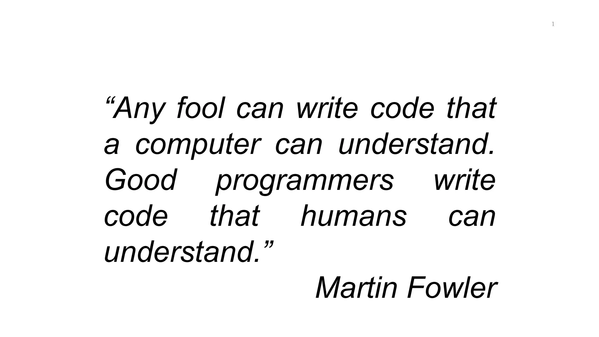
“Any fool can write code that
a computer can understand.
Good programmers write
code that humans can
understand.”
Martin Fowler
1
Data Structure & Algorithms
CS-2510
2
Engr. Syed Zaid Irshad
MS Software Engineering (2017)
BSc Computer System Engineering (2014)
3
Rules
 No use of Cell Phone (Except Emergency)
 Respect Boundaries
 Stay Clam and Cool
4
SubjectMarks
Total Marks: 100
Mid Term: 30
Final Term: 40
Class Participation:
Quizzes: Max 6, At least 4 Quizzes
Assignments: Max 6, At least 4 Assignments
5
Deadline
 Quizzes
 On Time: Obtained Marks
 After Due Time: Obtained Marks – 40%
 Assignments
 Till Due Date: Obtained Marks
 After Due Date: Obtained Marks – 40%
 Presentation/Quizzes/Assignments
 Max Time: May 28, 2022
6
Outline
 Intro to Data Structures and Algorithms
 Types of data and its nature
 DS operations
 Time-space trade-off
 How to write an algorithm
 Introduction to Asymptotic Notation and its
importance
 Abstract data types arrays
 ADT strings and their operations
 Introduction to Java
 Practical Implementation of Java
 Linear Search and Binary Search
 Polish notation
7
Outline
 Elementary Sorting techniques: Bubble, Selection,
Insertion
 Advance Sorting Techniques: Merge and Quick Sort,
Intro to Recursions
 Implementing algorithms through recursions
 Stacks, its operations, Polish notations
 Queues, Types of queues and their representation
 Link List (Single Linked List), Traversing, Insertion,
Updating and Deletion cases
 Doubly Linked List, Traversing, Insertion, updating
and deletion cases. Circular Linked List
 Sequential Search in Unordered Linked List
8
Outline
 Binary Search algorithm with Implementation & Intro
to Trees
 Binary Search Tree basic
 BST implementation, Traversing (BFS, DFS), Insert,
update and delete cases
 AVL trees Traversing, Insert, update and delete cases
 Graph Applications and algorithms, BFS, DFS, SPF
graphs
 Heap
 Hashing Tables
 Searching in Strings
9
Google
Classroom Code
AM: 3woxzla
BM: zwhxaf5
CM: se5a6lk
DM: sigjjwh
10
Your Turn
Introduce yourself
Name, Why picked this Subject, What you
Expect from me (except good marks)
11
Thinksyou
shouldKnow
 what is a programming language?
 how the instructions can be coded?
 how these instructions will be understood by the CPU
of computer so that they can be executed?
 Choose any language and try to get basics such as
 Data types & how memory is allocated to them
 Basic arithmetic like add, subtract etc.,
 Basic flows such as if, switch , loops etc.
 how control flows from one part of a program to another
 how to compile & run a program
 environments that support this programming language
 Basic Discrete Math's: Logic, Probability, Combination,
Algebra, Geometry, Topology
12
Why Learn DSA?
 To get an output you need two main things:
 Data
 Procedure
 To process the data using procedure you can do:
 Smart way
 Hard way
 If the scope of the problem is big you must
consider:
 How much Space it need?
 How much Time it will take?
13
Books
 Data Structures and Algorithms in C++ 4th
Edition- by Adam Drozdek
 Data Structures and algorithms by Goodrich,
4th edition.
 Algorithms by Robert and Wayne 4th edition.
14
DataStructures
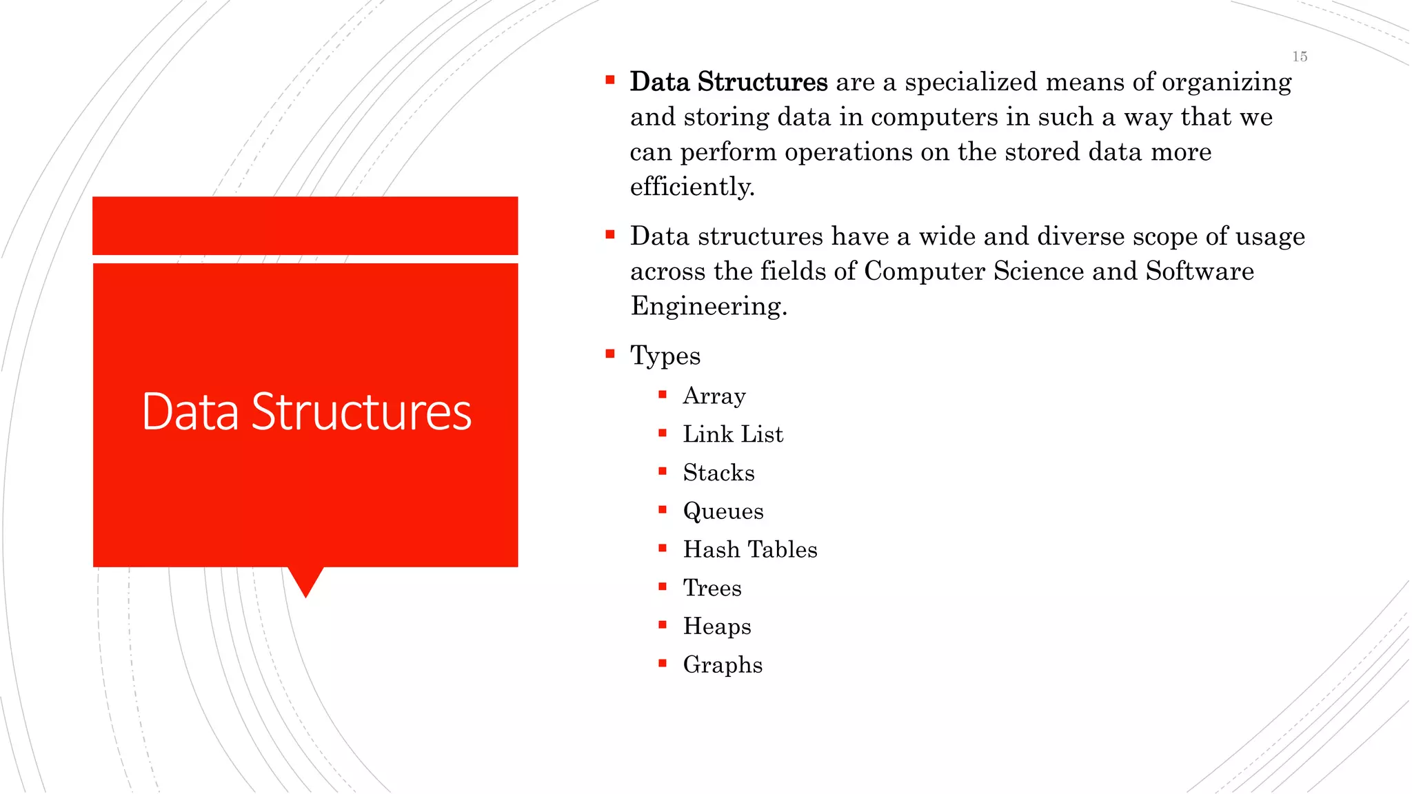
 Data Structures are a specialized means of organizing
and storing data in computers in such a way that we
can perform operations on the stored data more
efficiently.
 Data structures have a wide and diverse scope of usage
across the fields of Computer Science and Software
Engineering.
 Types
 Array
 Link List
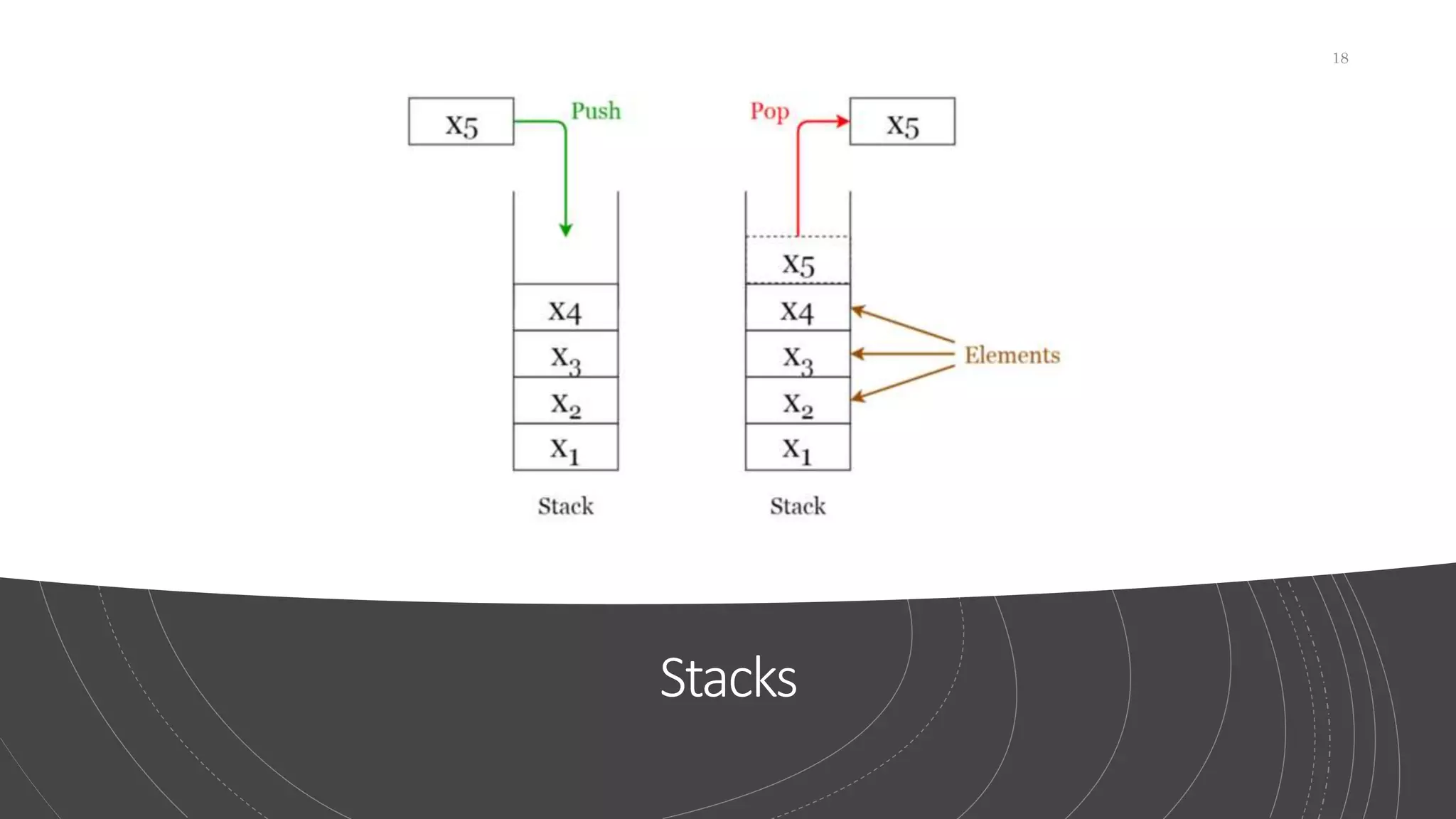
 Stacks
 Queues
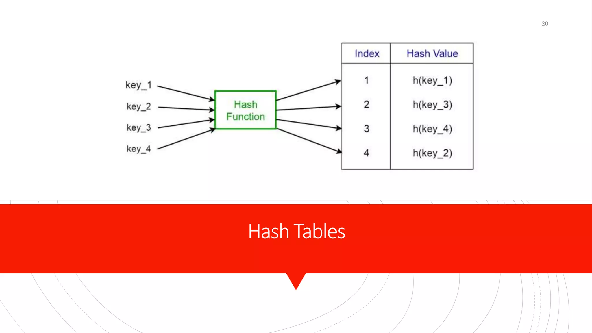
 Hash Tables
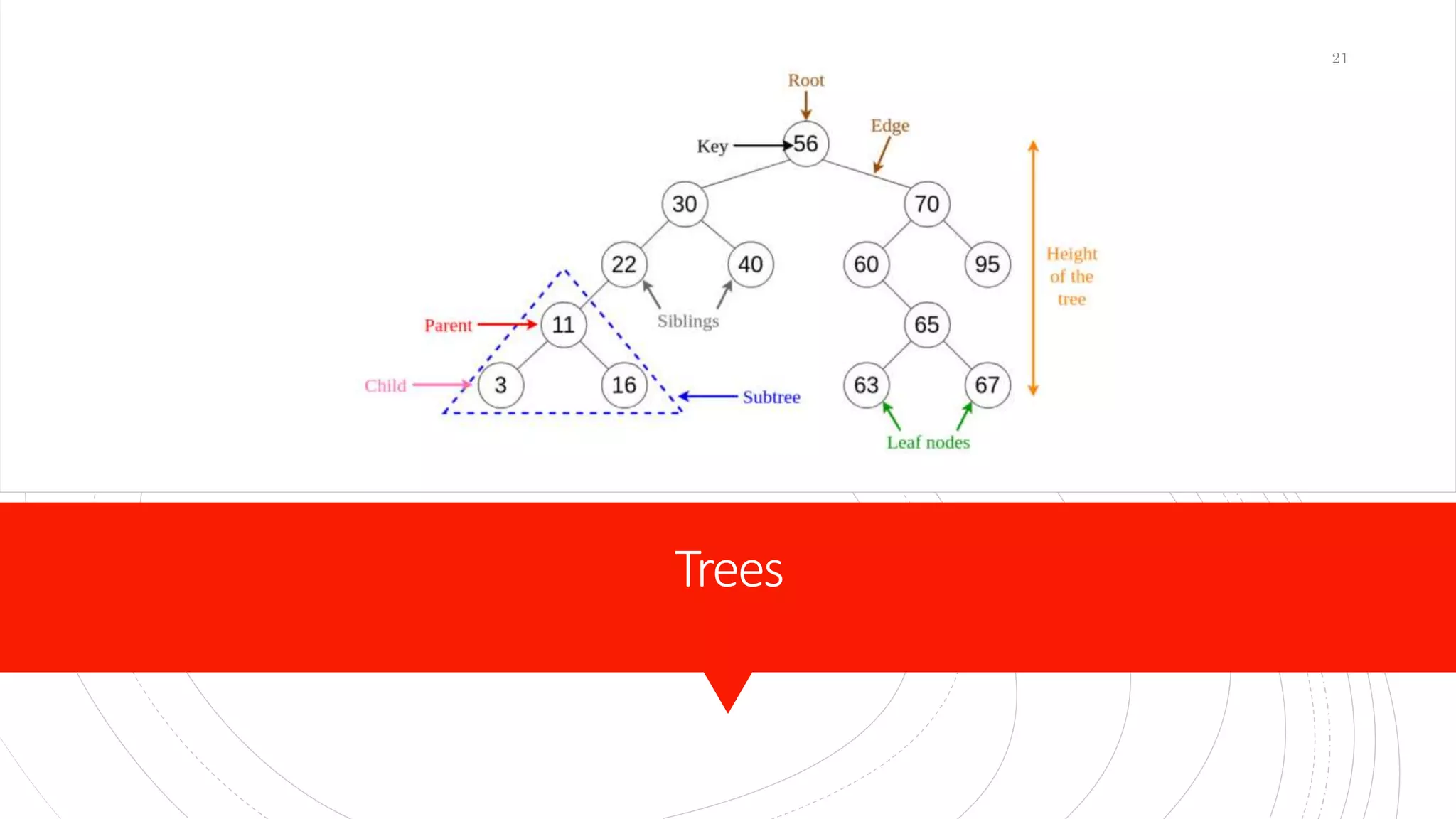
 Trees
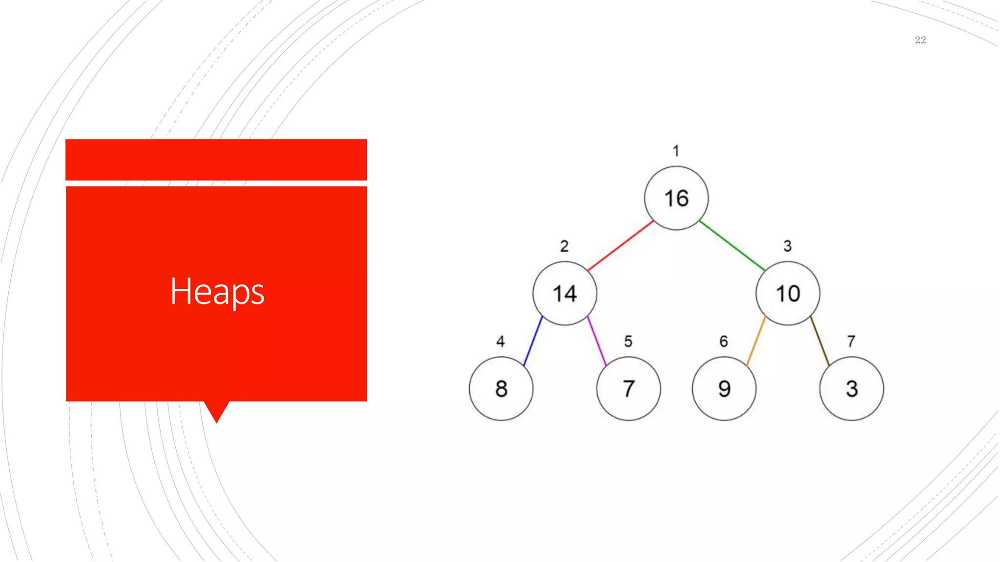
 Heaps
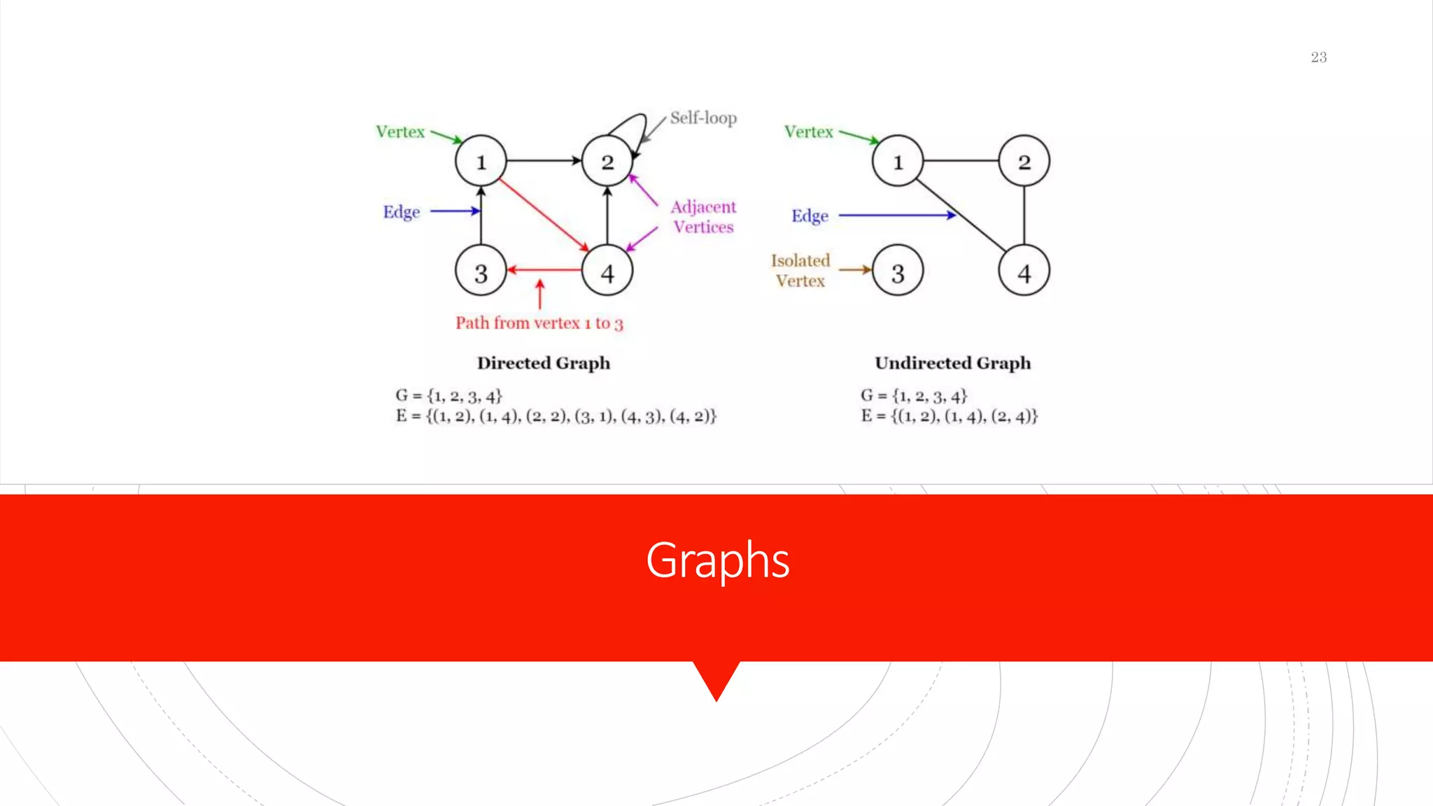
 Graphs
15
Array
16
LinkList
17
Stacks
18
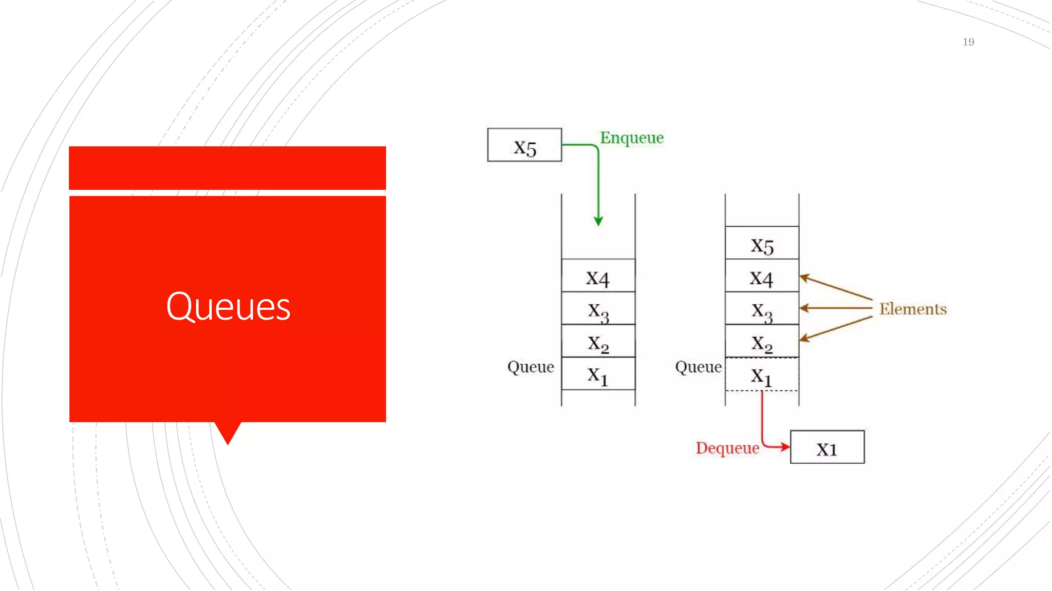
Queues
19
HashTables
20
Trees
21
Heaps
22
Graphs
23
Operations on
Data Structure
 There are four common operations that can
be performed:
 Traverse
 Search
 Insert
 Delete
24
“Before software can
be reusable it first
has to be usable.”
Ralph Johnson
25
Algorithm
 Algorithms are a step-by-step equation which makes
up a list of actions to perform a task in a program.
 Searching: Algorithms are used to search for an item
within the data.
 Sorting: Algorithms are used to sort different items
into a specific order.
 Inserting: Algorithms are used to insert items into the
data structure.
 Updating: Algorithms are used to update items in the
data structure.
 Deleting: Finally, algorithms can be used to delete
items from the data.
26
Trade-Off
 A tradeoff is a situation where one thing
increases, and another thing decreases.
 It is a way to solve a problem in:
 Either in less time and by using more space, or
 In very little space by spending a long amount of
time, or
 Making the right decision depending upon the
situation
 Types of Space-Time Trade-off
 Compressed or Uncompressed data
 Re Rendering or Stored images
 Smaller code or loop unrolling
 Lookup tables or Recalculation
27
Algorithm
Development
Process
 Step 1: Obtain a description of the problem.
 Step 2: Analyze the problem.
 Step 3: Develop a high-level algorithm.
 Step 4: Refine the algorithm by adding more detail.
 Step 5: Review the algorithm.
28
Obtaina
descriptionof
theproblem
 Defects that could be part of the description:
 The description relies on unstated assumptions
 The description is ambiguous
 The description is incomplete
 The description has internal contradictions
29
Analyzethe
problem
 Starting point
 What data are available?
 Where is that data?
 What formulas pertain to the problem?
 What rules exist for working with the data?
 What relationships exist among the data values?
 Ending point
 What new facts will we have?
 What items will have changed?
 What changes will have been made to those items?
 What things will no longer exist?
30
Developahigh-
levelalgorithm
 Problem: I need a send a birthday card to my brother, Mark.
 Analysis: I don't have a card. I prefer to buy a card rather than
make one myself.
 High-level algorithm:
 Go to a store that sells greeting cards
Select a card
Purchase a card
Mail the card
 This algorithm is satisfactory for daily use, but it lacks details
that would have to be added were a computer to carry out the
solution. These details include answers to questions such as the
following.
 "Which store will I visit?"
 "How will I get there: walk, drive, ride my bicycle, take the bus?"
 "What kind of card does Mark like: humorous, sentimental,
risqué?"
31
Refinethe
algorithmby
addingmoredetail
 A high-level algorithm shows the major steps that need
to be followed to solve a problem.
 Now we need to add details to these steps, but how
much detail should we add? Unfortunately, the answer
to this question depends on the situation.
 We must consider who (or what) is going to implement
the algorithm and how much that person (or thing)
already knows how to do.
 If someone is going to purchase Mark's birthday card
on my behalf, my instructions must be adapted to
whether that person is familiar with the stores in the
community and how well the purchaser knows my
brother's taste in greeting cards.
32
Reviewthe
algorithm
 Does this algorithm solve a very specific problem, or
does it solve a more general problem? If it solves a very
specific problem, should it be generalized?
 Can this algorithm be simplified?
 Is this solution like the solution to another problem?
How are they alike? How are they different?
33
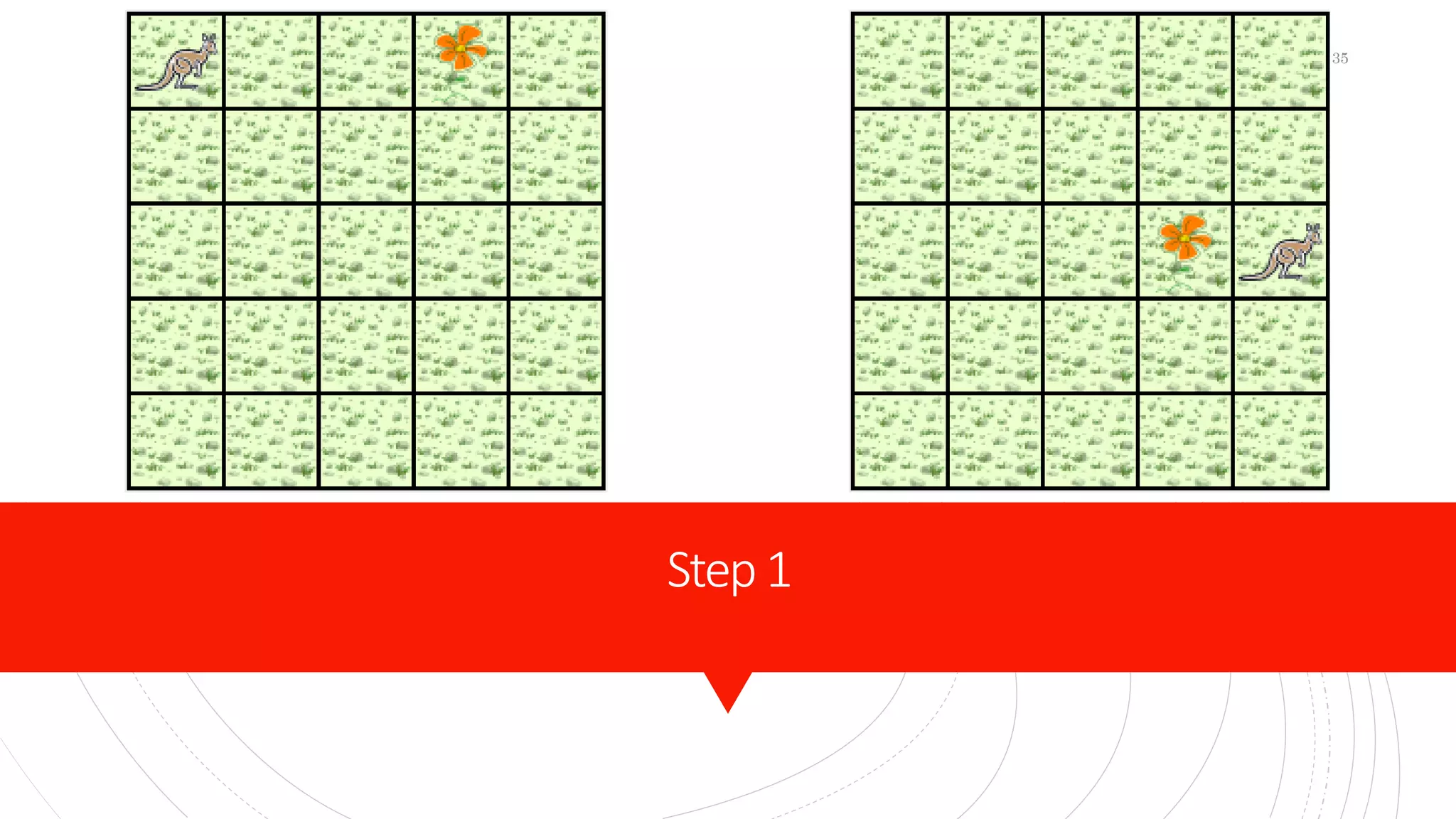
Example
 A Jeroo starts at (0, 0) facing East with no flowers in
its pouch. There is a flower at location (3, 0). Write a
program that directs the Jeroo to pick the flower and
plant it at a location (3, 2). After planting the flower,
the Jeroo should hop one space East and stop. There
are no other nets, flowers, or Jeroo's on the island.
34
Step1
35
Step2
 The flower is exactly three spaces ahead of the jeroo.
 The flower is to be planted exactly two spaces South of
its current location.
 The Jeroo is to finish facing East one space East of the
planted flower.
 There are no nets to worry about.
36
Step3
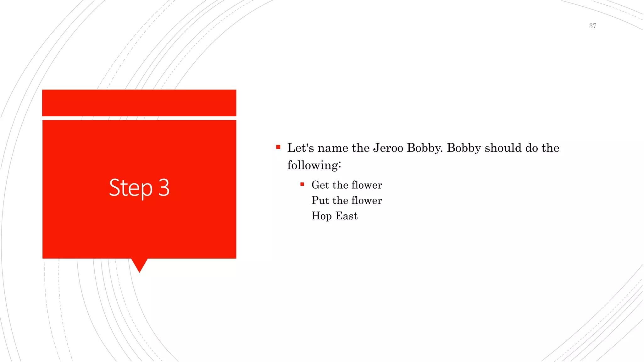
 Let's name the Jeroo Bobby. Bobby should do the
following:
 Get the flower
Put the flower
Hop East
37
Step4
 Let's name the Jeroo Bobby. Bobby should do the
following:
 Get the flower
 Hop 3 times
Pick the flower
 Put the flower
 Turn right Hop 2 times Plant a flower
 Hop East
 Turn left Hop once
38
Step5
 The high-level algorithm partitioned the problem into
three rather easy subproblems. This seems like a good
technique.
 This algorithm solves a very specific problem because
the Jeroo and the flower are in very specific locations.
 This algorithm is a solution to a slightly more general
problem in which the Jeroo starts anywhere, and the
flower is 3 spaces directly ahead of the Jeroo.
39
Asymptotic
Notations
 Asymptotic Notations are languages that allow us to
analyze an algorithm’s running time by identifying its
behavior as the input size for the algorithm increases.
 These notations invented by Paul Bachmann, Edmund
Landau, and others, collectively called Bachmann–
Landau notation or asymptotic notation.
 This is also known as an algorithm’s growth rate.
 Does the algorithm suddenly become incredibly slow
when the input size grows?
 Does it mostly maintain its quick run time as the input
size increases?
 Asymptotic Notation gives us the ability to answer
these questions.
40
Functionsof
GrowthRates
 Constant
 1
 Logarithmic Function
 log n
 Linear Function
 a*n + b
 Quadratic Function
 a*n^2 + bn + c
 Polynomial Function
 a*n^z + . . . + an^2 + a*n^1 + a*n^0
 Exponential Function
 a^n
41
Types
ofAsymptotic
Notations
 Big-O notation
 Omega notation
 Theta notation
42
Big-O
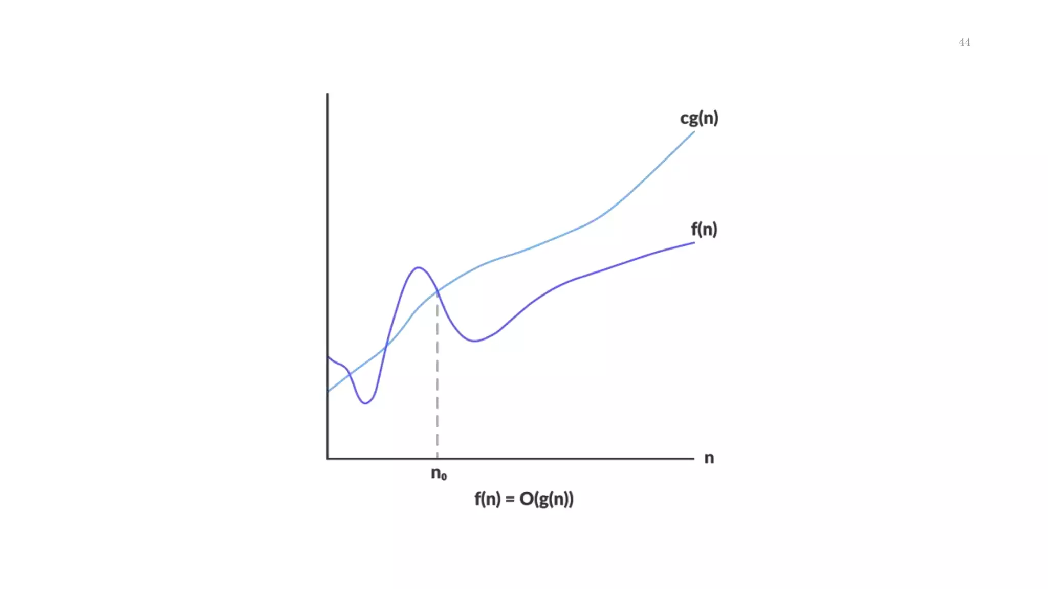
 Big O notation is a mathematical notation that
describes the limiting behavior of a function when the
argument tends towards a particular value or infinity.
 Big-O notation represents the upper bound of the
running time of an algorithm. Thus, it gives the worst-
case complexity of an algorithm.
 f(n) < c*g(n)
 For any value of n, the running time of an algorithm
does not cross the time provided by O(g(n)).
43
44
Stepsto figuring
outtheBigO
 Step #1: Count the steps
 Step #2: Different steps get added
 Step#3: Drop constants and coefficients
 Step#4: Drop non-dominant terms
 Step #5: Different inputs get different variables
45
Example  Let f(n)=3n4+2n2, find c*g(n) and write in O(g(n))
46
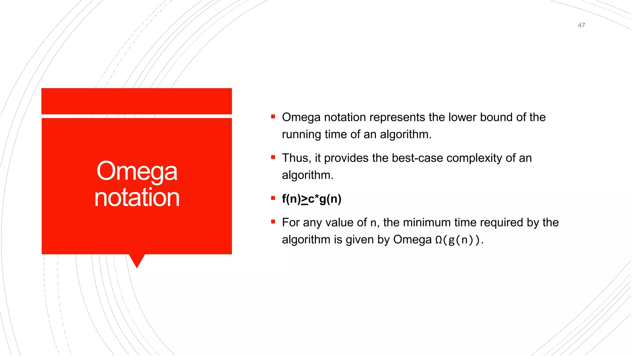
Omega
notation
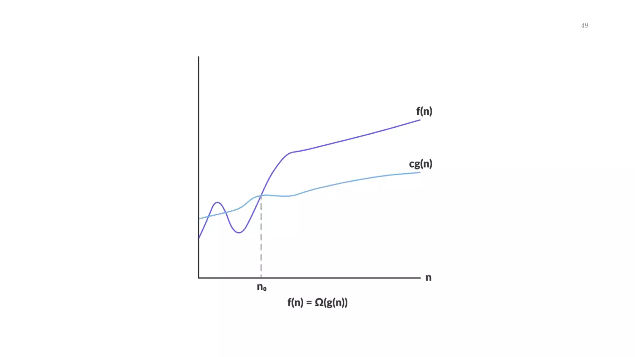
 Omega notation represents the lower bound of the
running time of an algorithm.
 Thus, it provides the best-case complexity of an
algorithm.
 f(n)>c*g(n)
 For any value of n, the minimum time required by the
algorithm is given by Omega Ω(g(n)).
47
48
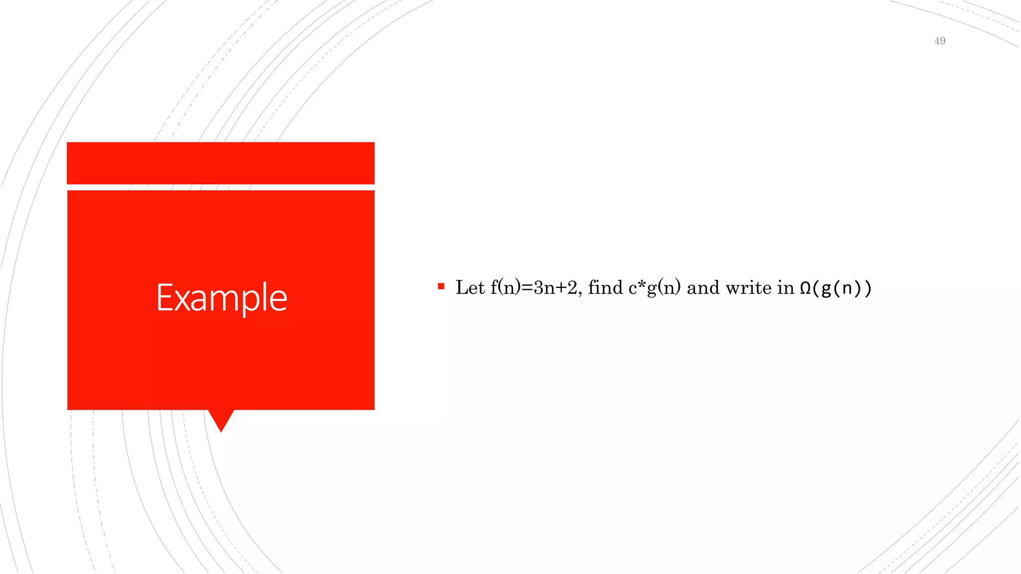
Example  Let f(n)=3n+2, find c*g(n) and write in Ω(g(n))
49
Measuring programming
progress by the lines of
code is like measuring
aircraft building progress
by weight.
50
Theta notation
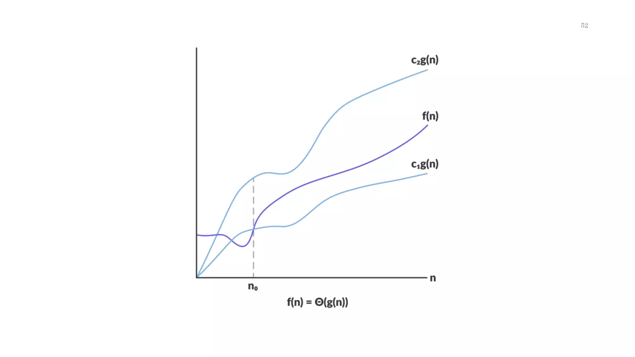
 Theta notation encloses the function from above and
below.
 c1*g(n)<f(n)<c2*g(n)
 Since it represents the upper and the lower bound of the
running time of an algorithm, it is used for analyzing the
average-case complexity of an algorithm.
51
52
Example
Let f(n)=10n3+3n+2,
find c1*g(n), c2*g(n) and write
in Theta(g(n))
53
AbstractData
Types
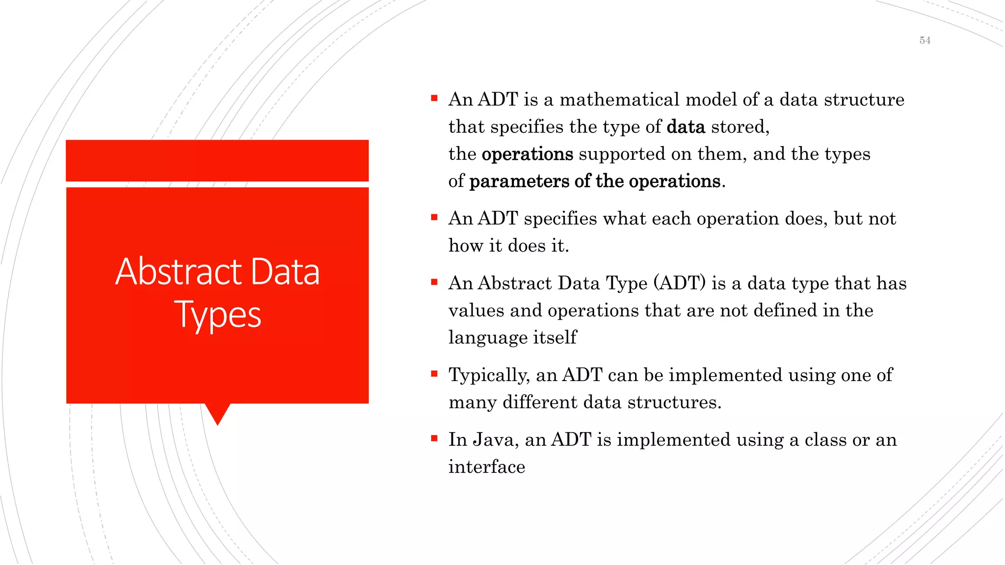
 An ADT is a mathematical model of a data structure
that specifies the type of data stored,
the operations supported on them, and the types
of parameters of the operations.
 An ADT specifies what each operation does, but not
how it does it.
 An Abstract Data Type (ADT) is a data type that has
values and operations that are not defined in the
language itself
 Typically, an ADT can be implemented using one of
many different data structures.
 In Java, an ADT is implemented using a class or an
interface
54
Abstract
DataTypes
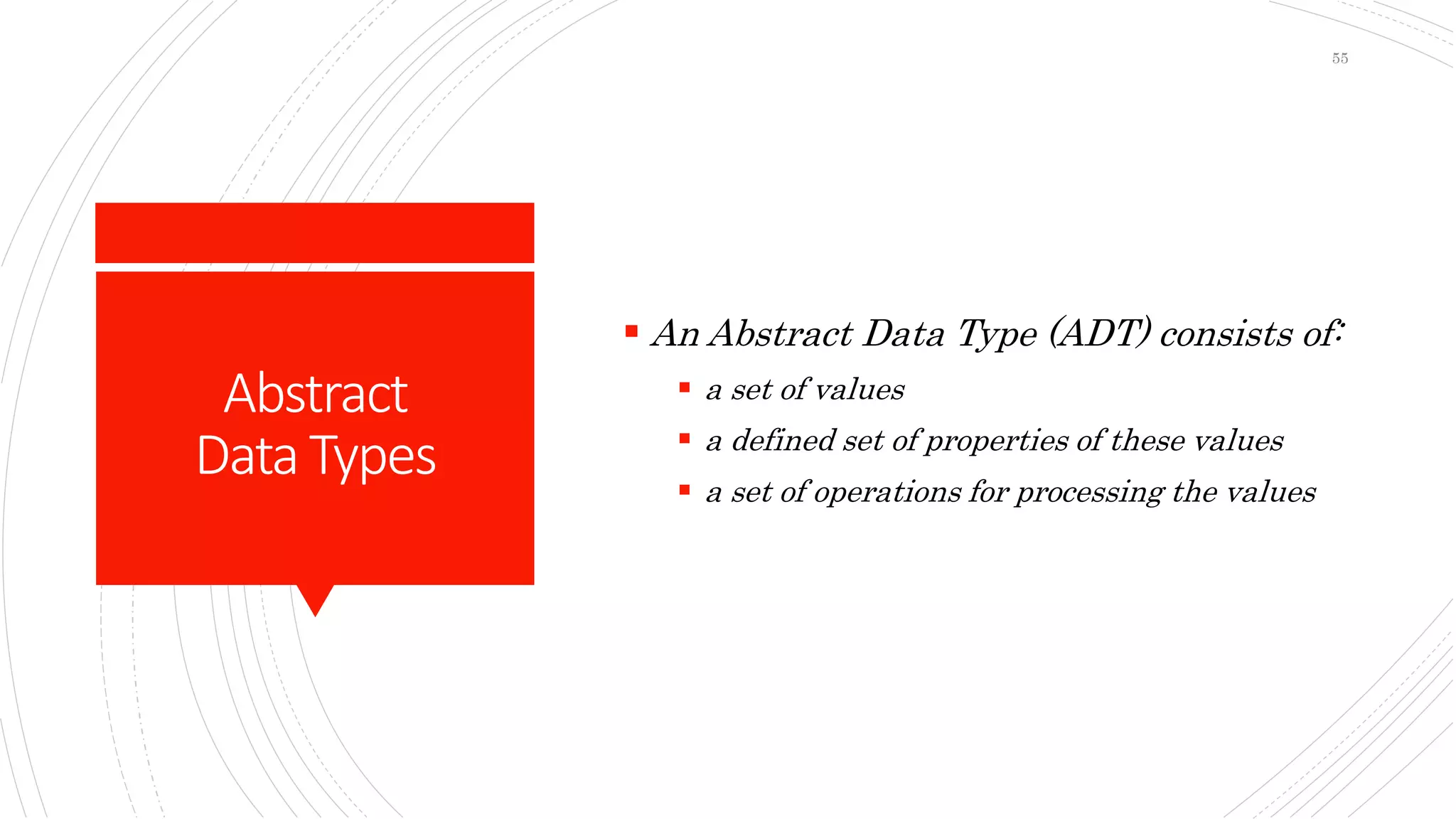
 An Abstract Data Type (ADT) consists of:
 a set of values
 a defined set of properties of these values
 a set of operations for processing the values
55
AbstractData
Types
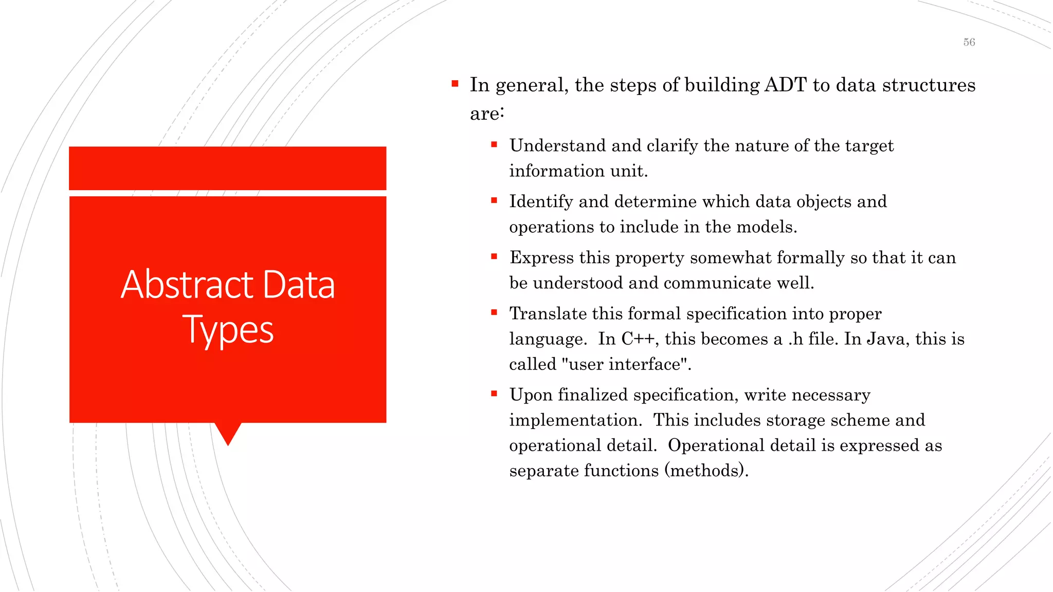
 In general, the steps of building ADT to data structures
are:
 Understand and clarify the nature of the target
information unit.
 Identify and determine which data objects and
operations to include in the models.
 Express this property somewhat formally so that it can
be understood and communicate well.
 Translate this formal specification into proper
language. In C++, this becomes a .h file. In Java, this is
called "user interface".
 Upon finalized specification, write necessary
implementation. This includes storage scheme and
operational detail. Operational detail is expressed as
separate functions (methods).
56
StringADT
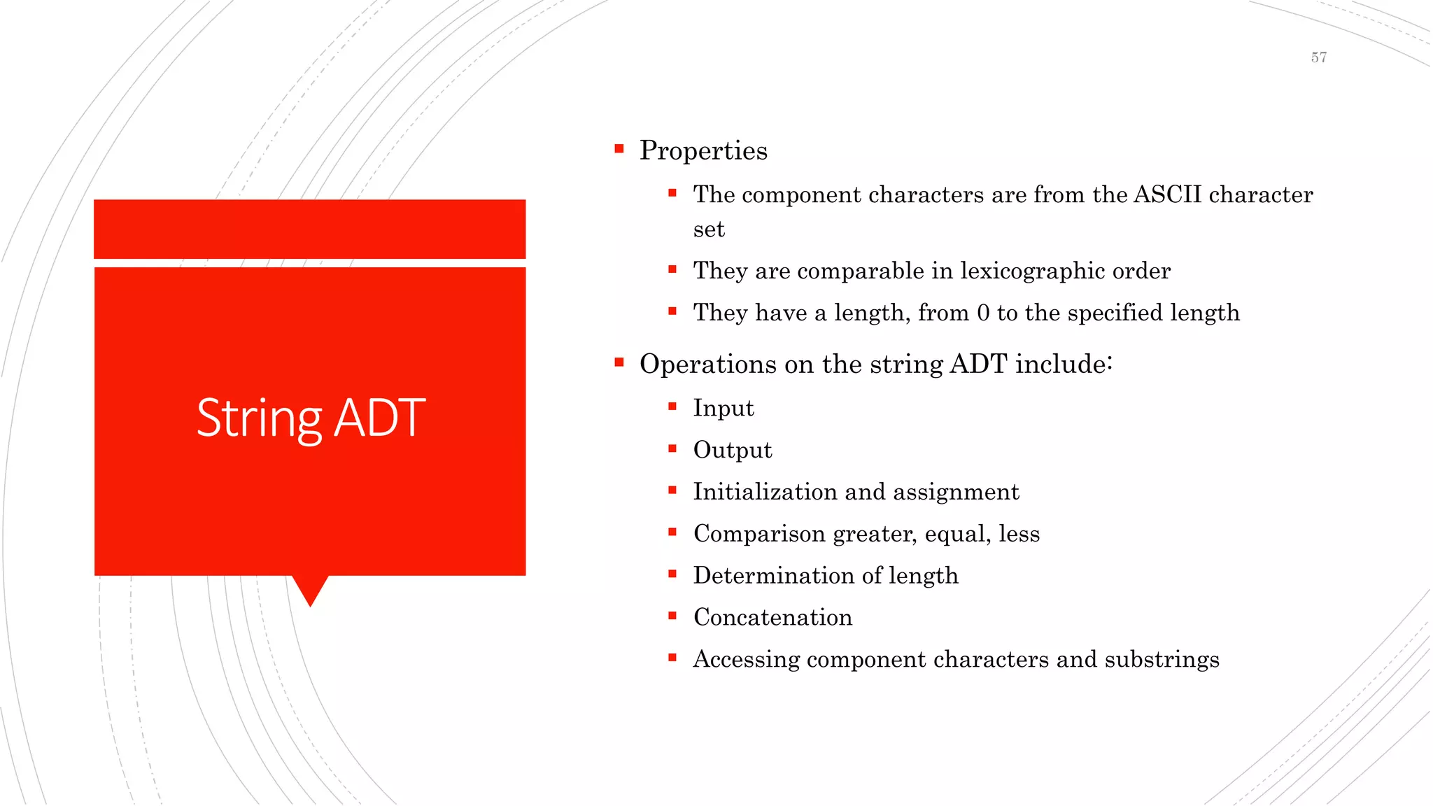
 Properties
 The component characters are from the ASCII character
set
 They are comparable in lexicographic order
 They have a length, from 0 to the specified length
 Operations on the string ADT include:
 Input
 Output
 Initialization and assignment
 Comparison greater, equal, less
 Determination of length
 Concatenation
 Accessing component characters and substrings
57
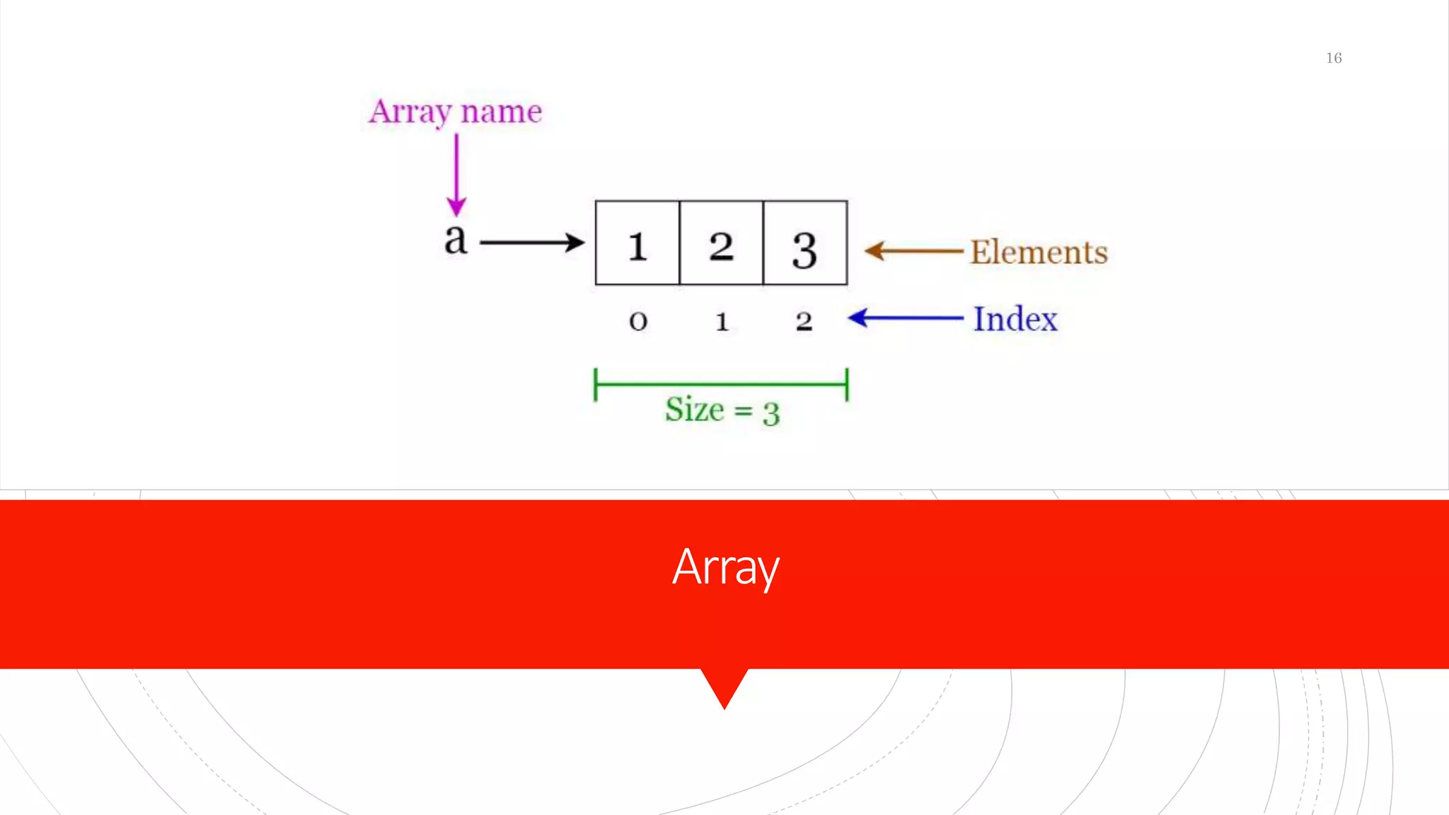
Array
 Properties:
 Linear Data Structure
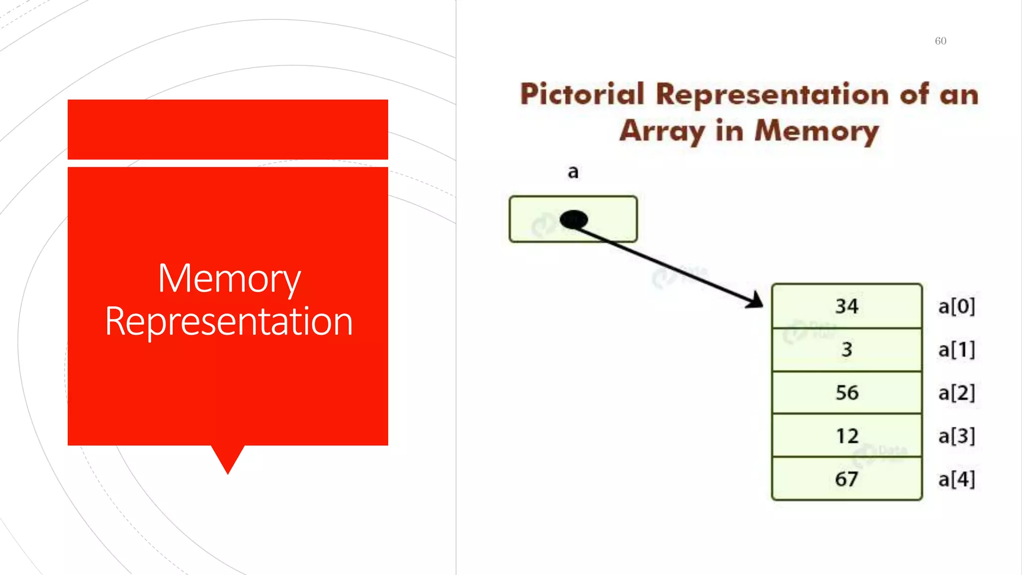
 Elements are stored in contiguous memory locations
 Can access elements randomly using index
 Stores homogeneous elements i.e., similar elements
 Syntax:
 Array declaration
 datatype var_name []=new datatype[size];
 datatype[] var_name=new datatype[size];
 Can also do declaration and initialization at once
 Datatype var_name [] = {ele1, ele2, ele3, ele4};
58
Array
 Advantages
 Random access
 Easy sorting and iteration
 Replacement of multiple variables
 Disadvantages
 Size is fixed
 Difficult to insert and delete
 If capacity is more and occupancy less, most of the array
gets wasted
 Needs contiguous memory to get allocated
 Applications
 For storing information in a linear fashion
 Suitable for applications that require frequent searching
59
Memory
Representation
60
Demonstration
ofArray
package array;
import java.util.*;
public class Array {
public static void main(String[] args) {
int[] priceOfPen= new int[5];
Scanner in=new Scanner(System.in);
for(int i=0;i<priceOfPen.length;i++)
{
System.out.print("Enter pen "+i+" price: ");
priceOfPen[i]=in.nextInt();
}
for(int i=0;i<priceOfPen.length;i++)
System.out.print(priceOfPen[i]+" ");
}
}
61
Stack
 Properties:
 Linear Data Structures using Java
 Follows LIFO: Last In First Out
 Only the top elements are available to be accessed
 Insertion and deletion takes place from the top
 I.e., a stack of plates, chairs, etc.
 Basic Operations of Stack
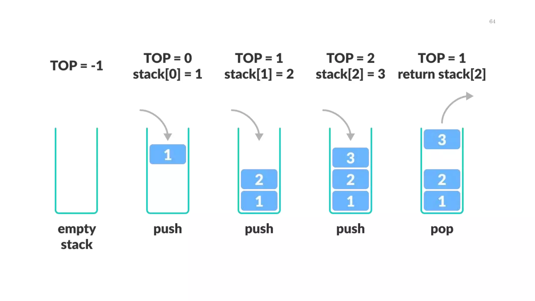
 Push: Add an element to the top of a stack
 Pop: Remove an element from the top of a stack
 IsEmpty: Check if the stack is empty
 IsFull: Check if the stack is full
 Peek: Get the value of the top element without removing
it
62
Stack
 Advantages
 Maintains data in a LIFO manner
 The last element is readily available for use
 All operations are of O(1) complexity
 Disadvantages
 Manipulation is restricted to the top of the stack
 Not much flexible
 Applications
 Recursion
 Parsing
 Browser
 Editors
63
64
Demonstration
ofStack
(Create)
private final int arr[];
private int top;
private final int capacity;
// Creating a stack
Stack(int size) {
arr = new int[size];
capacity = size;
top = -1;
}
65
Demonstration
ofStack
(State)
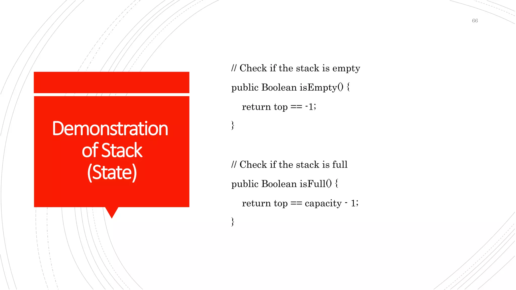
// Check if the stack is empty
public Boolean isEmpty() {
return top == -1;
}
// Check if the stack is full
public Boolean isFull() {
return top == capacity - 1;
}
66
Demonstration
ofStack
(Push)
// Add elements into stack
public void push(int x) {
if (isFull()) {
System.out.println("OverFlownProgram
Terminatedn");
System.exit(1);
}
System.out.println("Inserting " + x);
arr[++top] = x;
}
67
Demonstration
ofStack
(Pop)
// Remove element from stack
public int pop() {
if (isEmpty()) {
System.out.println("STACK EMPTY");
System.exit(1);
}
return arr[top--];
}
68
Demonstration
ofStack
(Peek)
// Display without removing element from stack
public int peek() {
if (isEmpty()) {
System.out.println("STACK EMPTY");
System.exit(1);
}
return arr[top];
}
69
Demonstration
ofStack
(Print)
public void printStack() {
for (int i = 0; i <= top; i++) {
System.out.println(arr[i]);
}
}
70
Demonstration
ofStack
(Main)
public static void main(String[] args) {
Stack stack = new Stack(5);
stack.push(1);
stack.push(2);
stack.push(3);
stack.push(4);
stack.pop();
System.out.println("nAfter popping out");
stack.printStack();
stack.peek();
System.out.println("nAfter peeking");
stack.printStack();
}
71
PolishNotation
 Polish notation is a notation form for expressing
arithmetic, logic and algebraic equations.
 Its most basic distinguishing feature is that operators
are placed on the left of their operands.
 If the operator has a defined fixed number of operands,
the syntax does not require brackets or parenthesis to
lessen ambiguity.
 Polish notation is also known as prefix notation, prefix
Polish notation, normal Polish notation, Warsaw
notation and Lukasiewicz notation.
72
Types
 Infix Notation
 We write expression in infix notation, e.g., a - b + c
 Prefix Notation
 In this notation, operator is prefixed to operands, i.e.
operator is written ahead of operands. For example, +ab.
This is equivalent to its infix notation a + b. Prefix
notation is also known as Polish Notation.
 Postfix Notation
 This notation style is known as Reversed Polish
Notation. In this notation style, the operator is postfixed
to the operands i.e., the operator is written after the
operands. For example, ab+. This is equivalent to its
infix notation a + b.
73
PostfixNotation
 Step 1: Add '')" to the end of the infix expression
 Step 2: Push ( onto the stack
 Step 3: Repeat until each character in the infix notation is scanned
 IF a ( is encountered, push it on the stack
 IF an operand (whether a digit or a character) is encountered, add it postfix
expression.
 IF a ")" is encountered, then
a. Repeatedly pop from stack and add it to the postfix expression until a "("
is encountered.
b. Discard the "(".That is, remove the(from stack and do not add it to the
postfix expression
 IF an operator O is encountered, then
a. Repeatedly pop from stack and add each operator ( popped from the stack)
to the postfix expression which has the same precedence or a higher
precedence than O
b. Push the operator to the stack
 [END OF IF]
 Step 4: Repeatedly pop from the stack and add it to the postfix
expression until the stack is empty
 Step 5: EXIT
74
Without requirements or
design, programming is
the art of adding bugs to
an empty text file.
75
PrefixNotation
 Step 1: Reverse the infix string. Note that while
reversing the string you must interchange left and
right parentheses.
 Step 2: Obtain the postfix expression of the infix
expression Step 1.
 Step 3: Reverse the postfix expression to get the prefix
expression
76
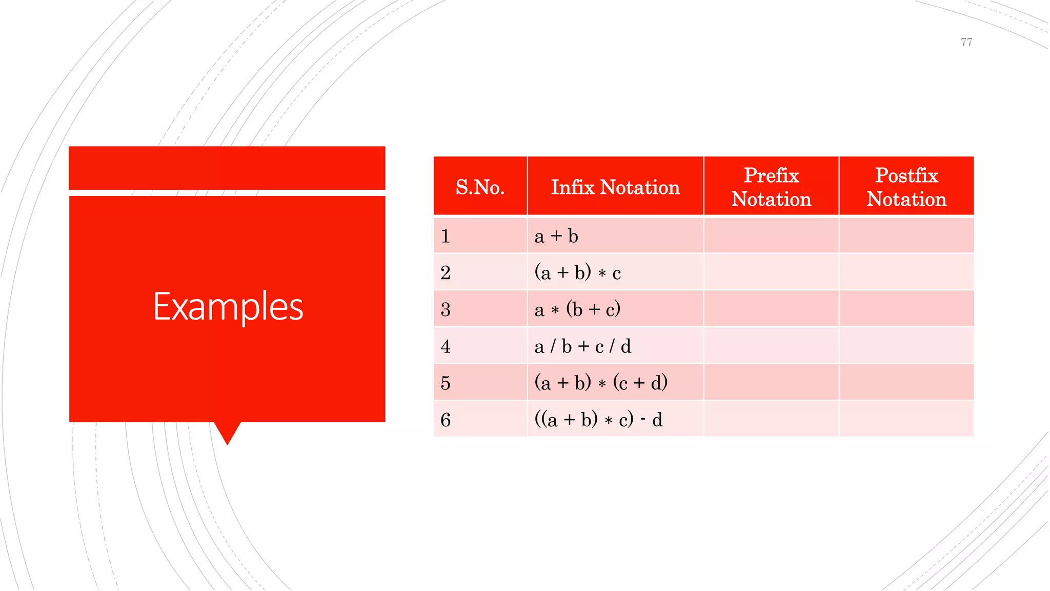
Examples
S.No. Infix Notation
Prefix
Notation
Postfix
Notation
1 a + b
2 (a + b) ∗ c
3 a ∗ (b + c)
4 a / b + c / d
5 (a + b) ∗ (c + d)
6 ((a + b) ∗ c) - d
77
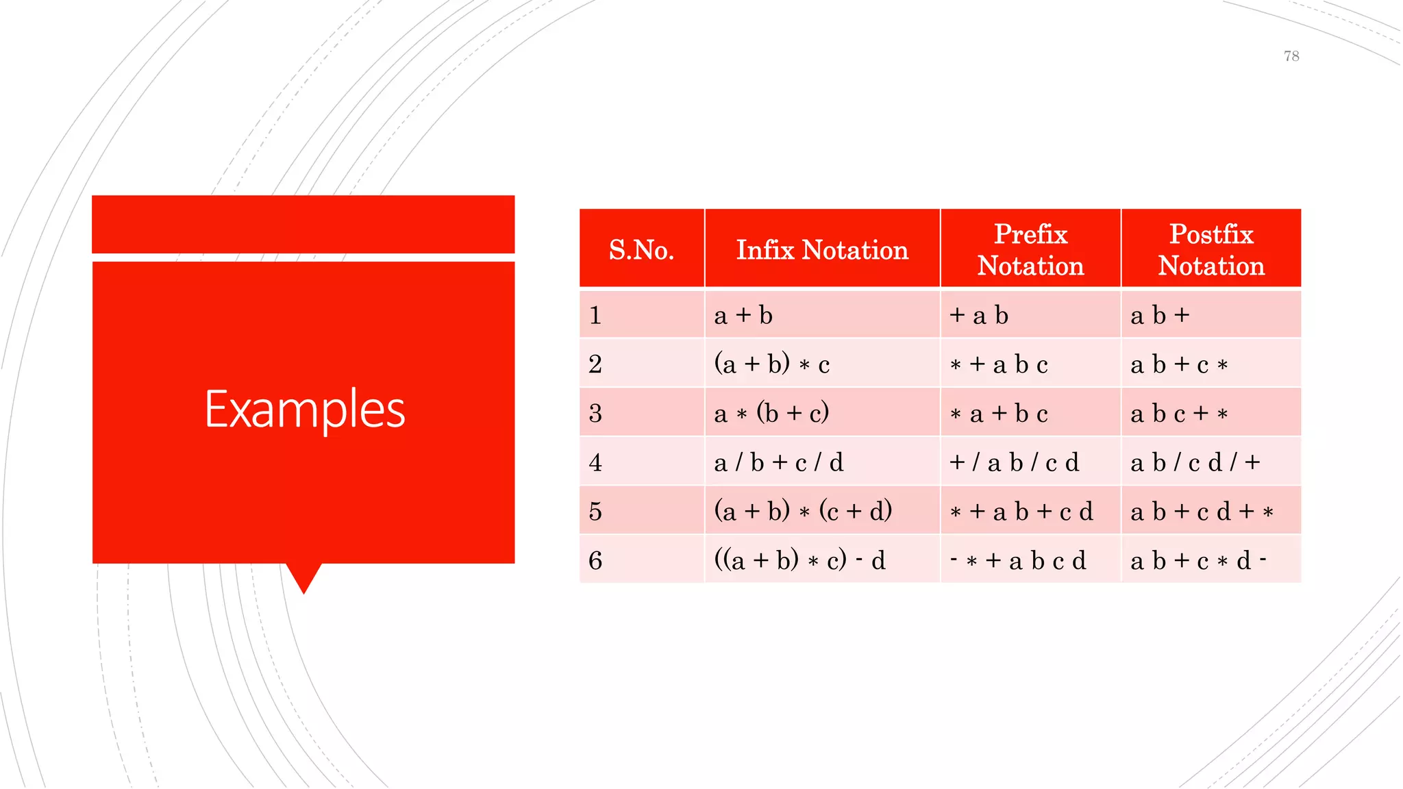
Examples
S.No. Infix Notation
Prefix
Notation
Postfix
Notation
1 a + b + a b a b +
2 (a + b) ∗ c ∗ + a b c a b + c ∗
3 a ∗ (b + c) ∗ a + b c a b c + ∗
4 a / b + c / d + / a b / c d a b / c d / +
5 (a + b) ∗ (c + d) ∗ + a b + c d a b + c d + ∗
6 ((a + b) ∗ c) - d - ∗ + a b c d a b + c ∗ d -
78
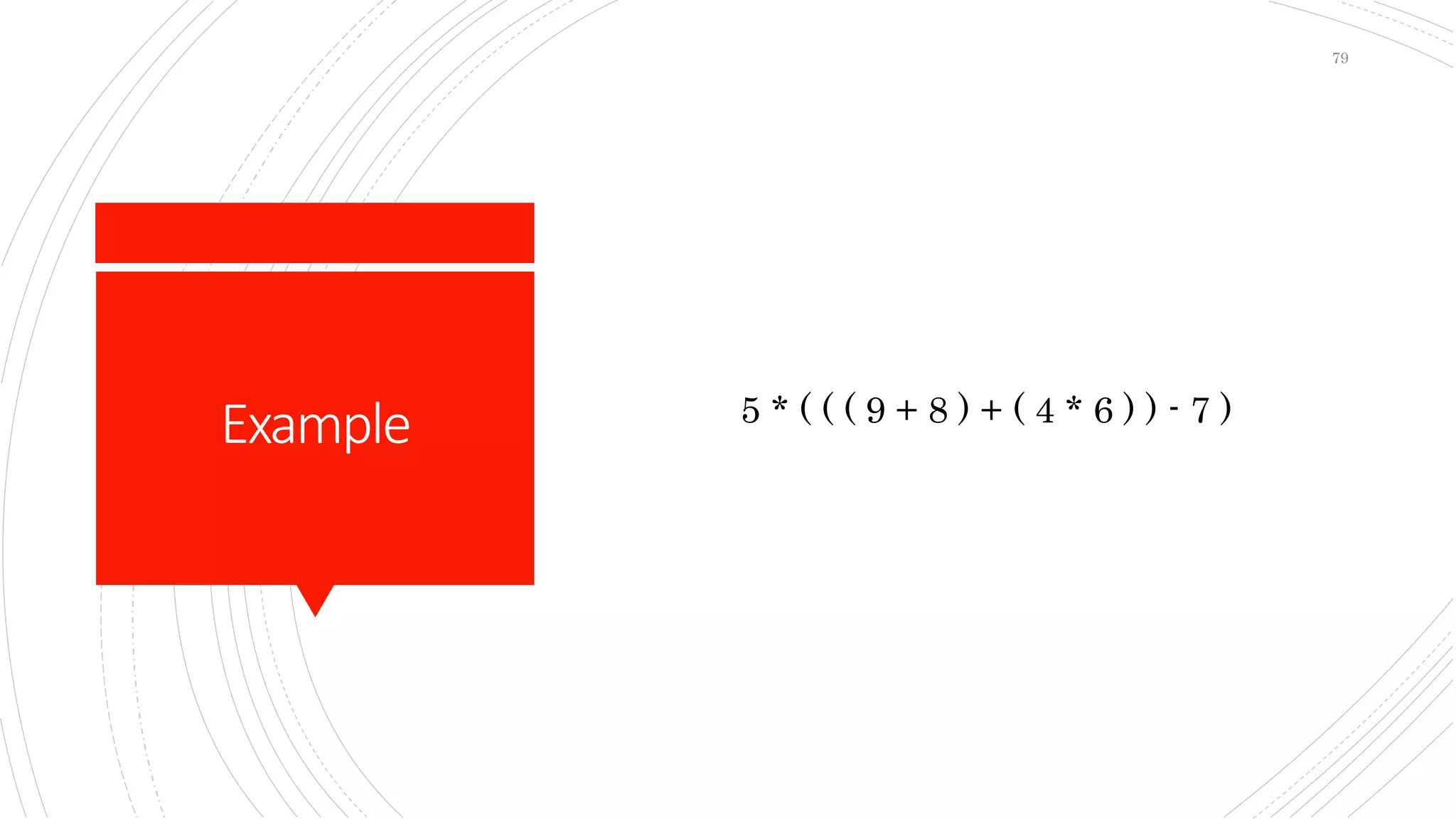
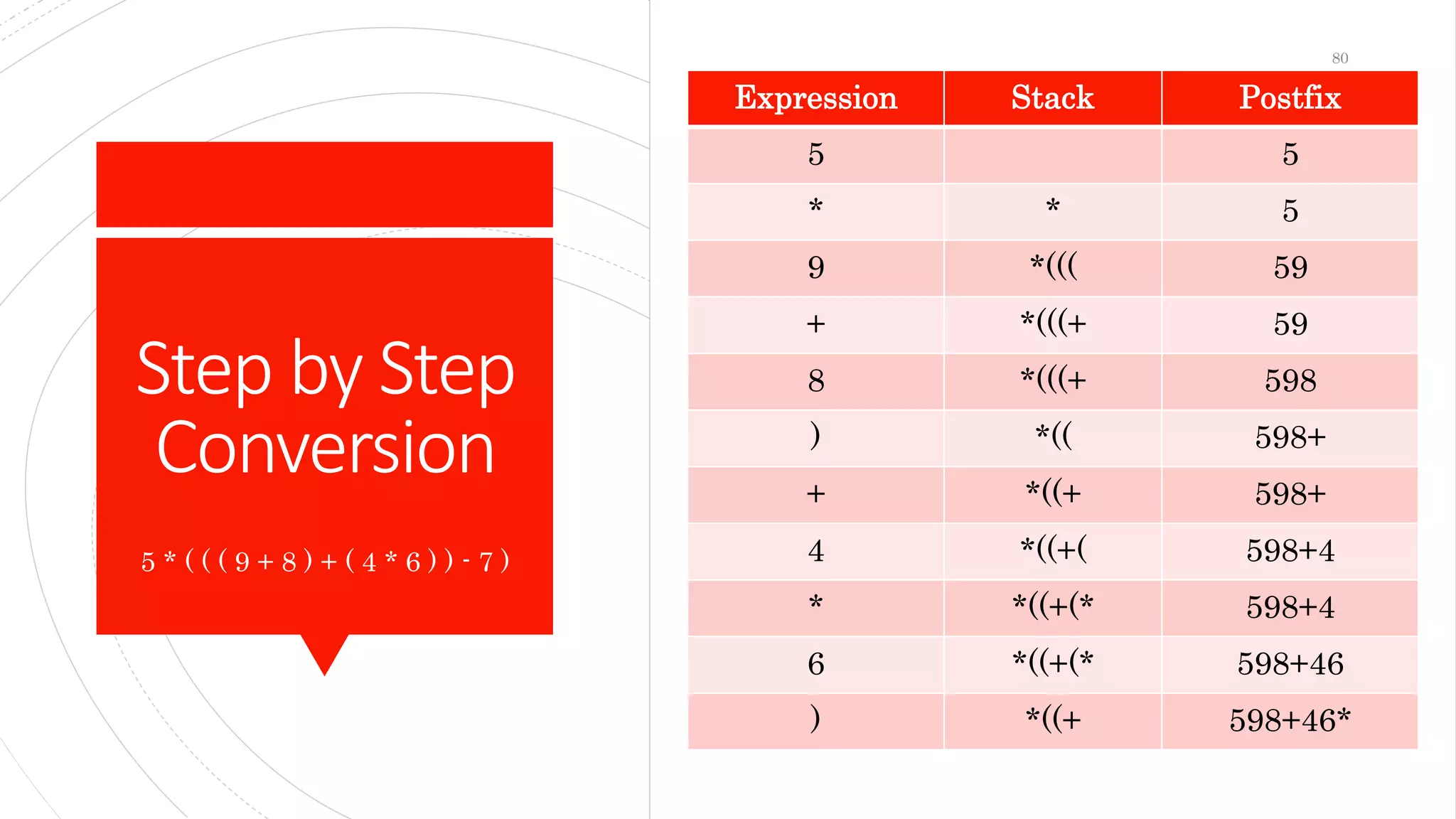
Example 5 * ( ( ( 9 + 8 ) + ( 4 * 6 ) ) - 7 )
79
Step by Step
Conversion
5 * ( ( ( 9 + 8 ) + ( 4 * 6 ) ) - 7 )
Expression Stack Postfix
5 5
* * 5
9 *((( 59
+ *(((+ 59
8 *(((+ 598
) *(( 598+
+ *((+ 598+
4 *((+( 598+4
* *((+(* 598+4
6 *((+(* 598+46
) *((+ 598+46*
80
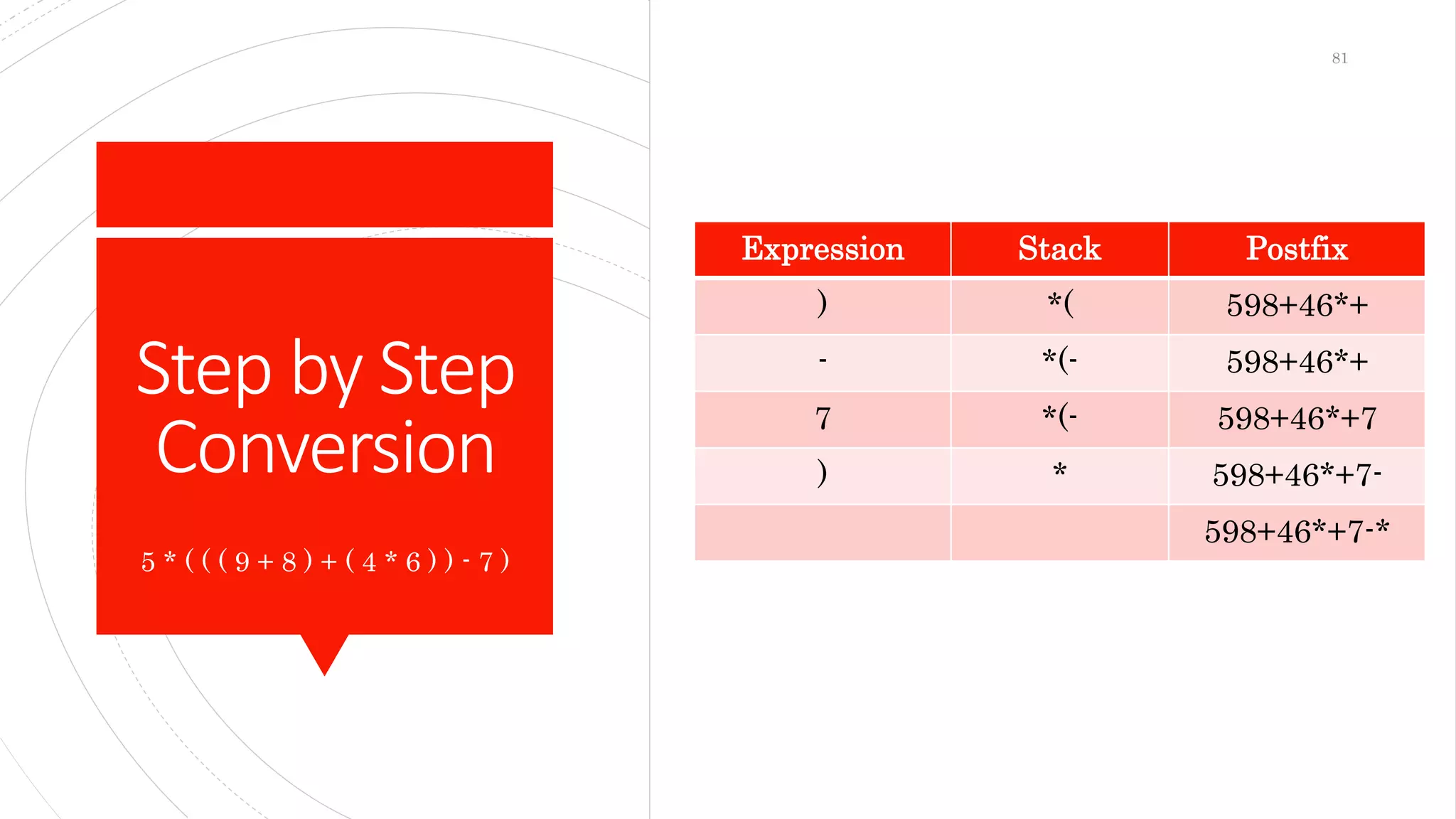
Step by Step
Conversion
5 * ( ( ( 9 + 8 ) + ( 4 * 6 ) ) - 7 )
Expression Stack Postfix
) *( 598+46*+
- *(- 598+46*+
7 *(- 598+46*+7
) * 598+46*+7-
598+46*+7-*
81
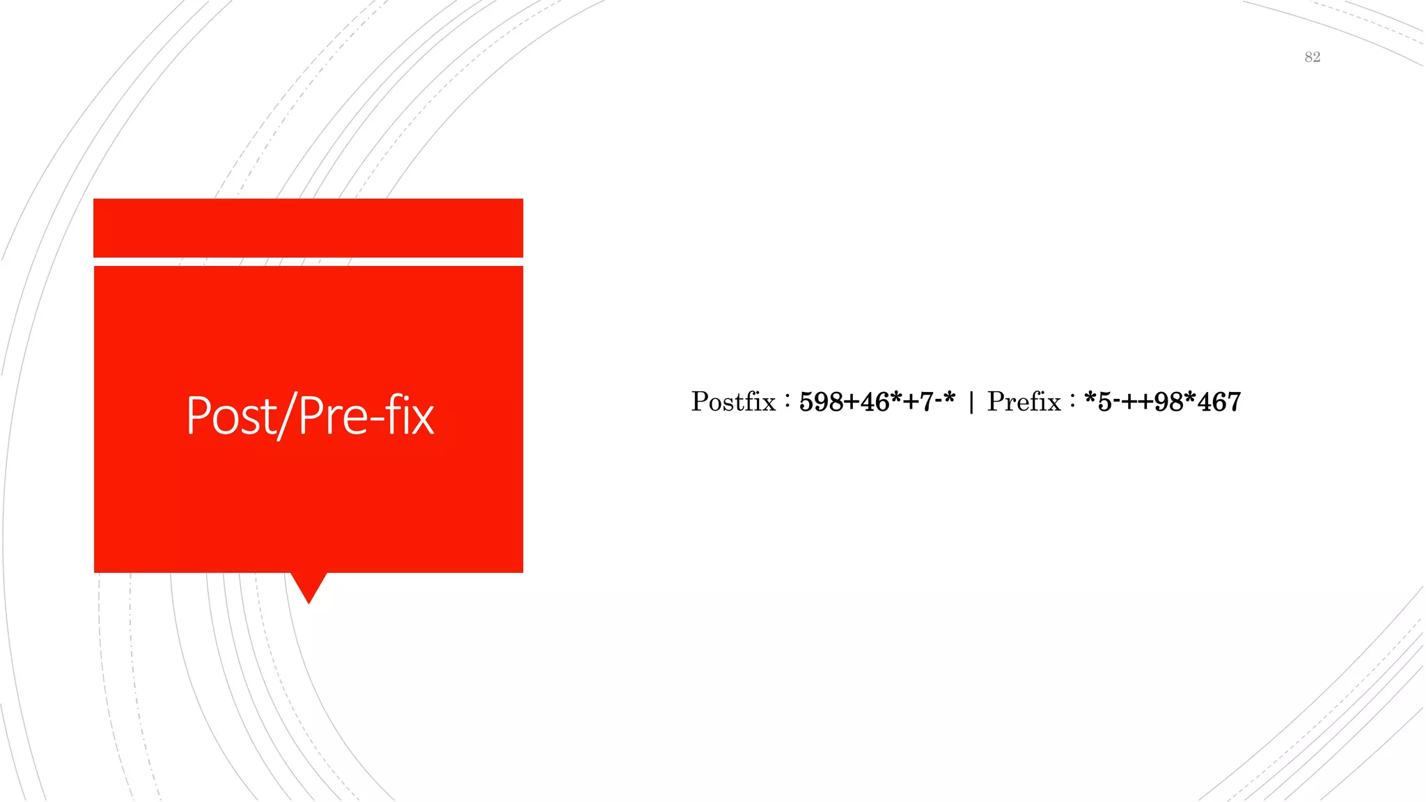
Post/Pre-fix Postfix : 598+46*+7-* | Prefix : *5-++98*467
82
Example
 Postfix form : 5 9 8 + 4 6 * + 7 - *
 Push( 5 ) Push( 9 ) Push( 8 )
 Push( Pop() + Pop() )
 Push( 4 ) Push( 6 )
 Push( Pop() * Pop() )
 Push( Pop() + Pop() )
 Push( 7 )
 Push( Pop() - Pop() )
 Push( Pop() * Pop() )
 Answer: 170
83
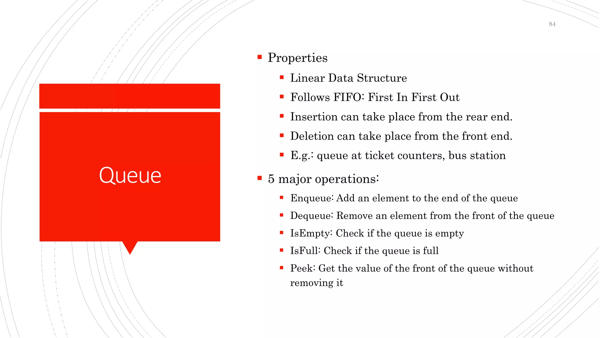
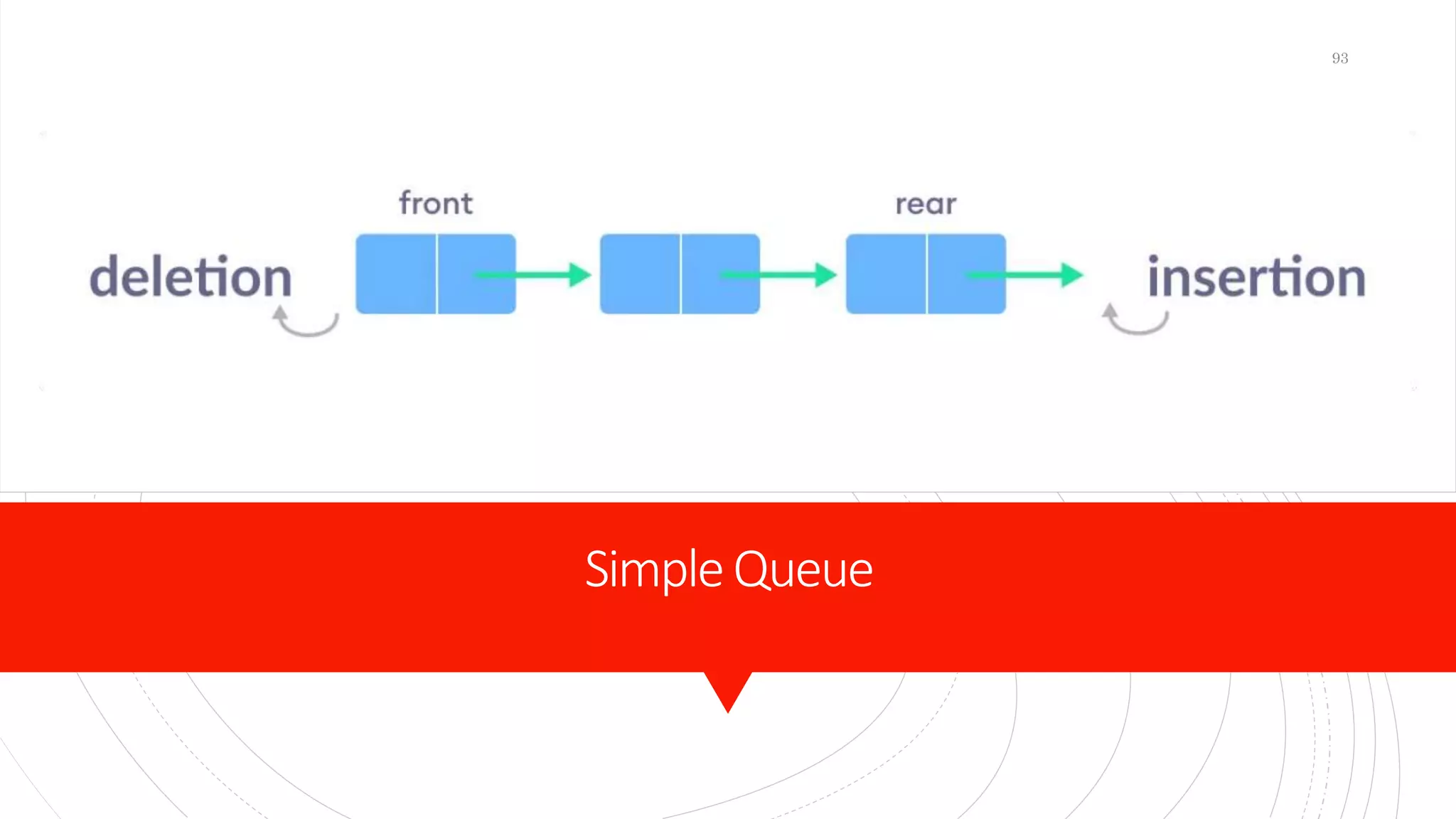
Queue
 Properties
 Linear Data Structure
 Follows FIFO: First In First Out
 Insertion can take place from the rear end.
 Deletion can take place from the front end.
 E.g.: queue at ticket counters, bus station
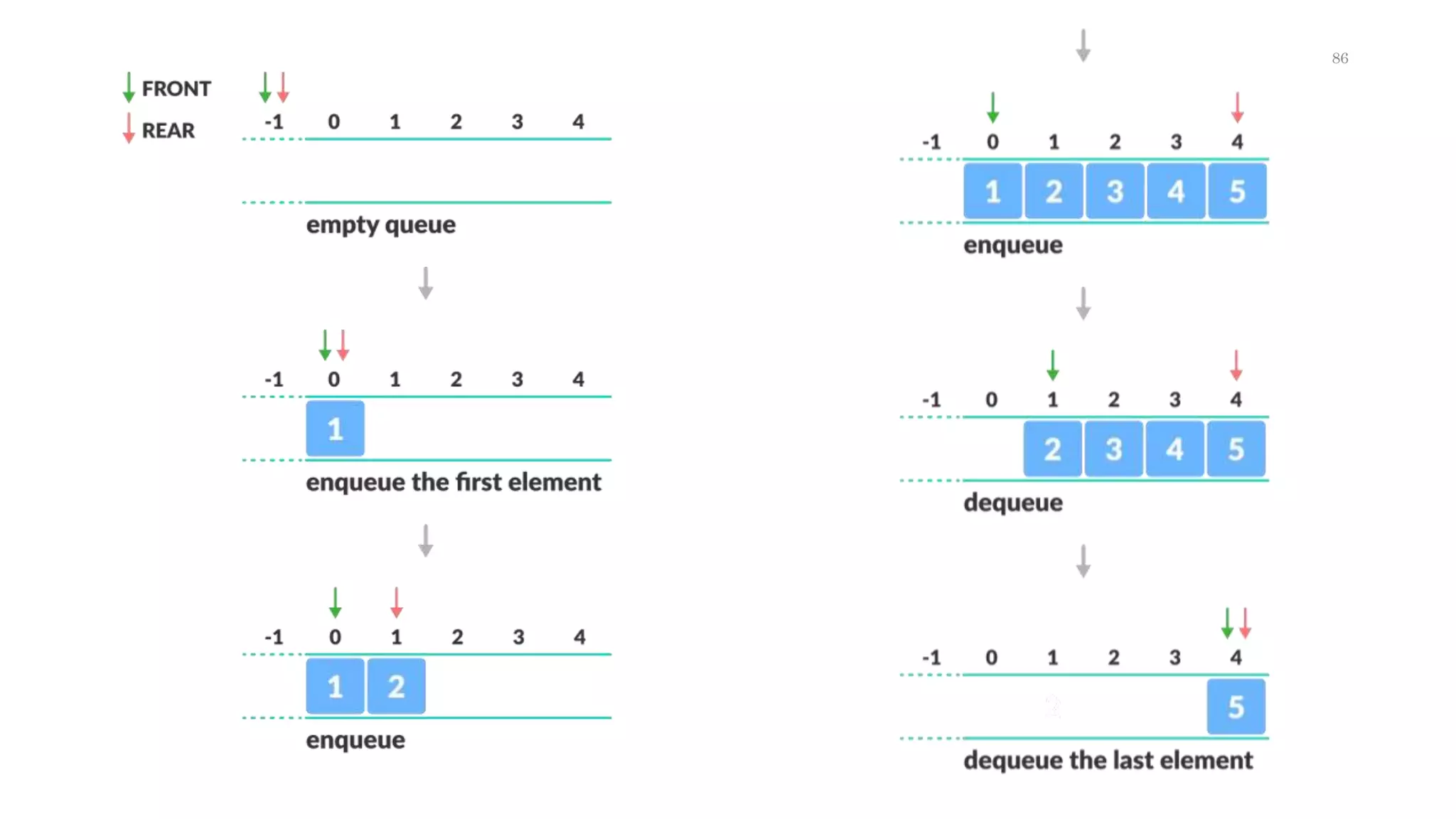
 5 major operations:
 Enqueue: Add an element to the end of the queue
 Dequeue: Remove an element from the front of the queue
 IsEmpty: Check if the queue is empty
 IsFull: Check if the queue is full
 Peek: Get the value of the front of the queue without
removing it
84
Queue
 Advantages
 Maintains data in FIFO manner
 Insertion from beginning and deletion from end
takes O(1) time
 Applications
 Scheduling
 Maintaining playlist
 Interrupt handling
85
86
Demonstration
ofQueue
(Create)
int SIZE = 5;
int items[] = new int[SIZE];
int front, rear;
Queue() {
front = -1;
rear = -1;
}
87
Demonstration
ofQueue
(State)
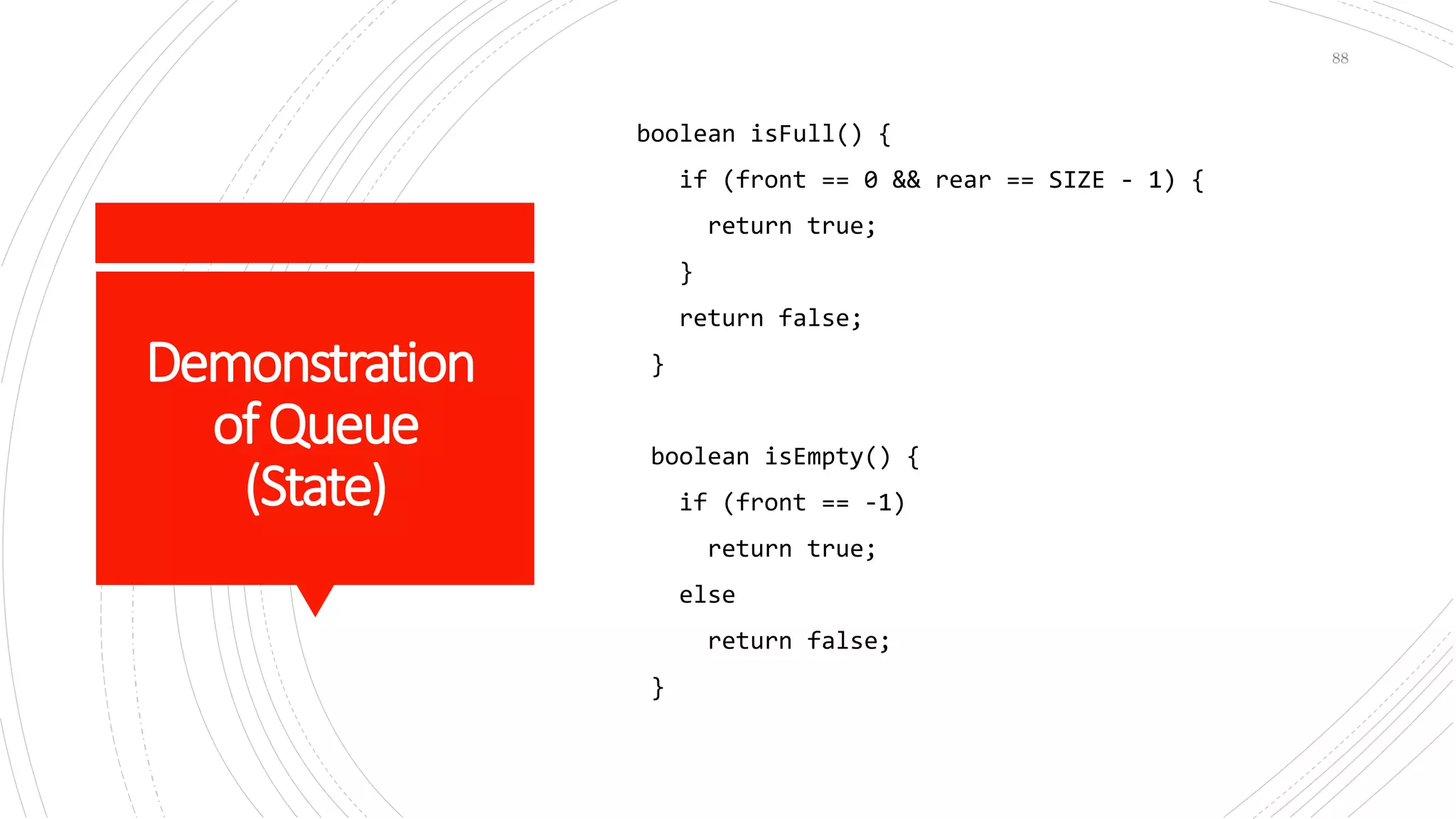
boolean isFull() {
if (front == 0 && rear == SIZE - 1) {
return true;
}
return false;
}
boolean isEmpty() {
if (front == -1)
return true;
else
return false;
}
88
Demonstration
ofQueue
(Enqueue)
void enQueue(int element) {
if (isFull()) {
System.out.println("Queue is full");
} else {
if (front == -1)
front = 0;
rear++;
items[rear] = element;
System.out.println("Inserted " + element);
}
}
89
Demonstration
ofQueue
(Dequeue)
if (isEmpty()) {
System.out.println("Queue is empty");
return (-1);
} else {
element = items[front];
if (front >= rear) {
front = -1;
rear = -1;
}
else {
front++;
}
System.out.println("Deleted -> " +
element);
return (element);
90
Demonstration
ofQueue
(Main)
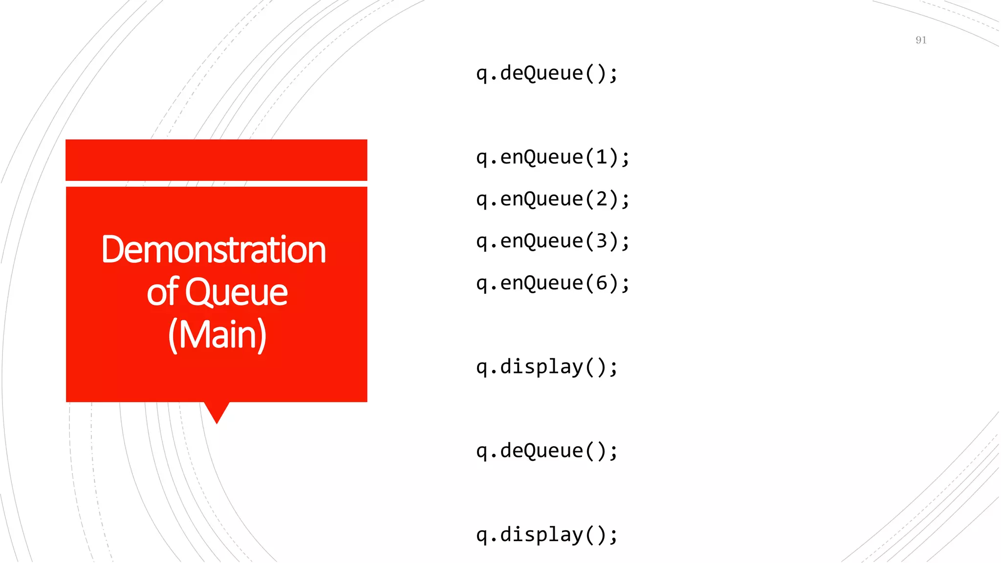
q.deQueue();
q.enQueue(1);
q.enQueue(2);
q.enQueue(3);
q.enQueue(6);
q.display();
q.deQueue();
q.display();
91
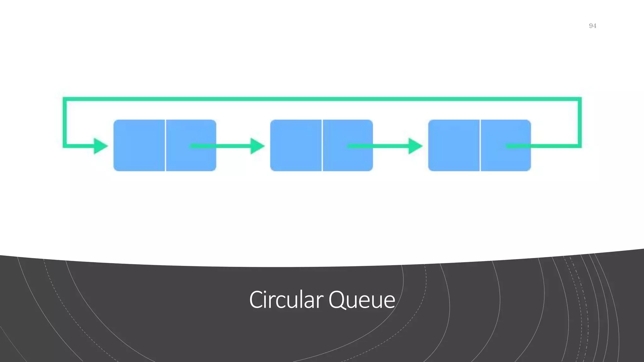
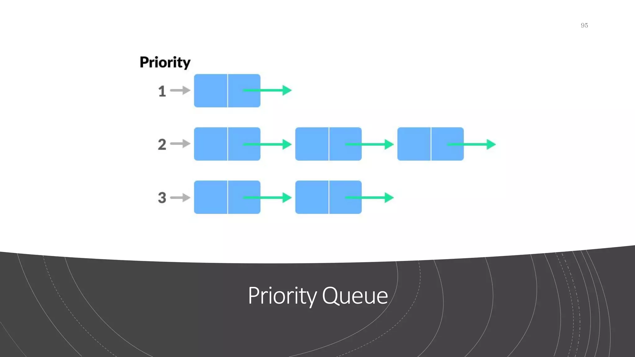
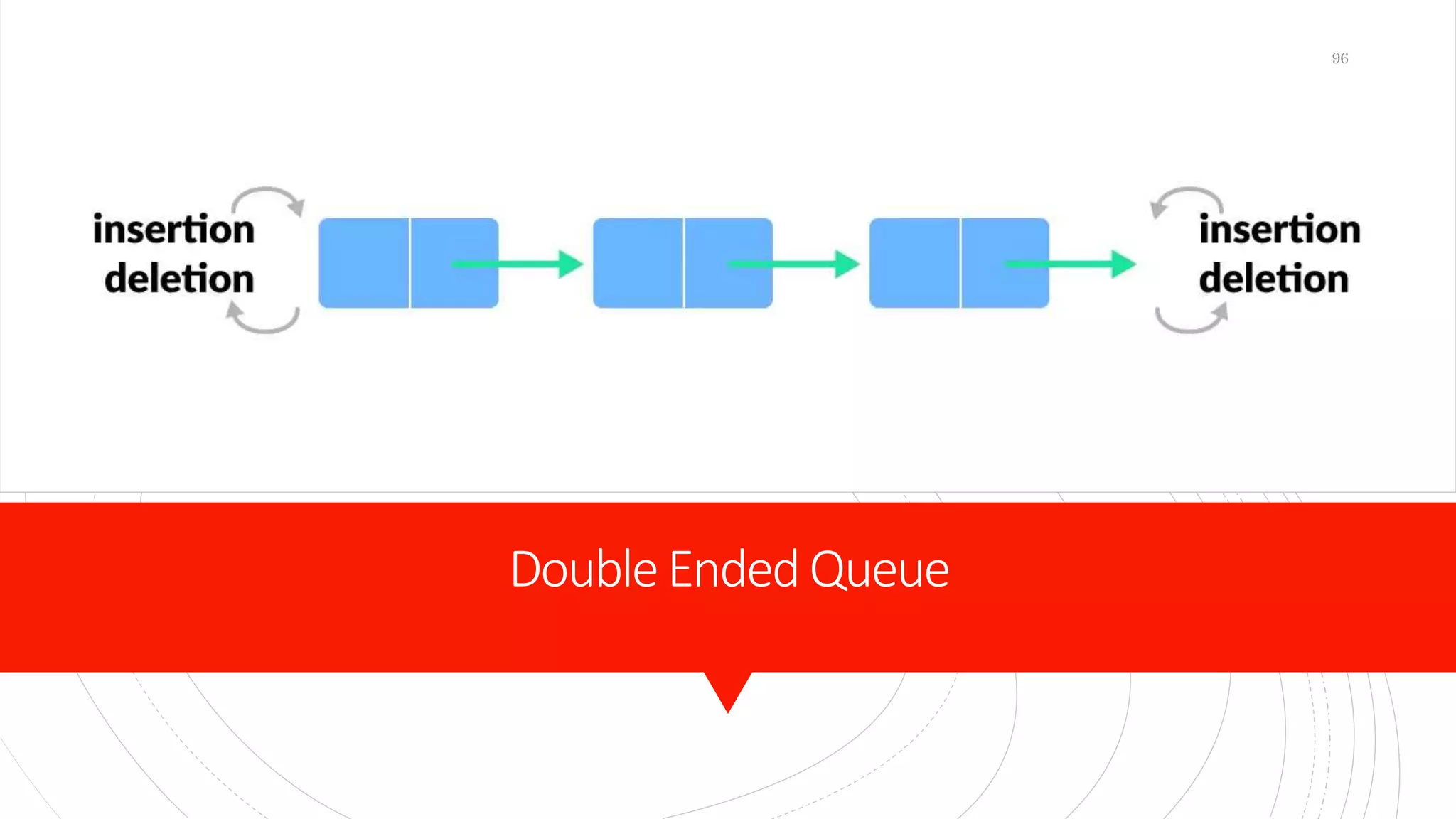
Typesof Queue
 There are four different types of queues:
 Simple Queue
 Circular Queue
 Priority Queue
 Double Ended Queue
92
SimpleQueue
93
CircularQueue
94
PriorityQueue
95
DoubleEndedQueue
96
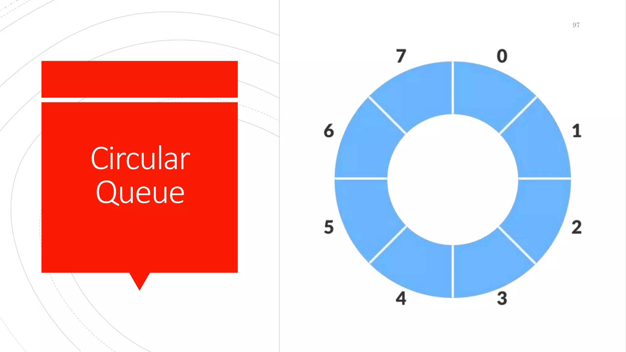
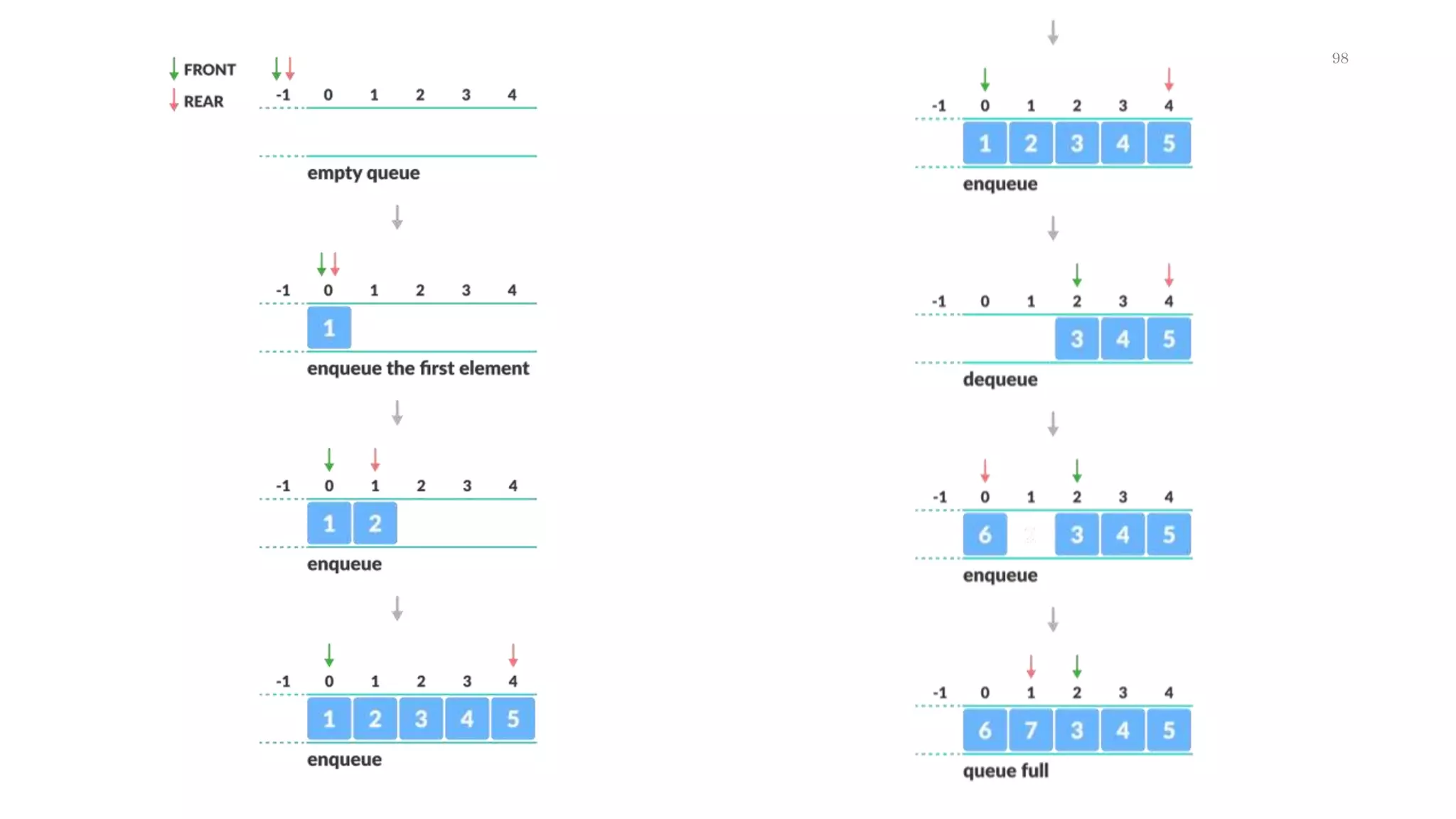
Circular
Queue
97
98
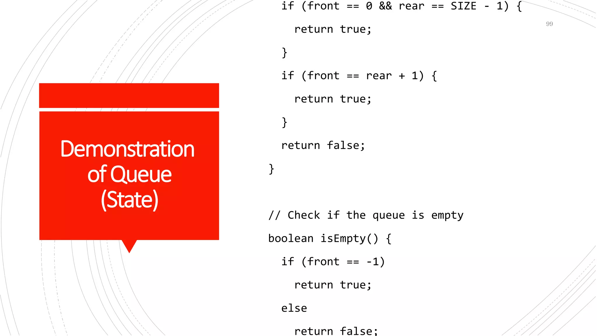
Demonstration
ofQueue
(State)
if (front == 0 && rear == SIZE - 1) {
return true;
}
if (front == rear + 1) {
return true;
}
return false;
}
// Check if the queue is empty
boolean isEmpty() {
if (front == -1)
return true;
else
return false;
99
"Programming isn't about
what you know; it's about
what you can figure out.”
Chris Pine
100
Demonstration
ofQueue
(Enqueue)
void enQueue(int element) {
if (isFull()) {
System.out.println("Queue is full");
} else {
if (front == -1)
front = 0;
rear = (rear + 1) % SIZE;
items[rear] = element;
System.out.println("Inserted " + element);
}
}
101
Demonstration
ofQueue
(Dequeue)
int element;
if (isEmpty()) {
System.out.println("Queue is empty");
return (-1);
} else {
element = items[front];
if (front == rear) {
front = -1;
rear = -1;
}
else {
front = (front + 1) % SIZE;
}
return (element);
}
102
PriorityQueue
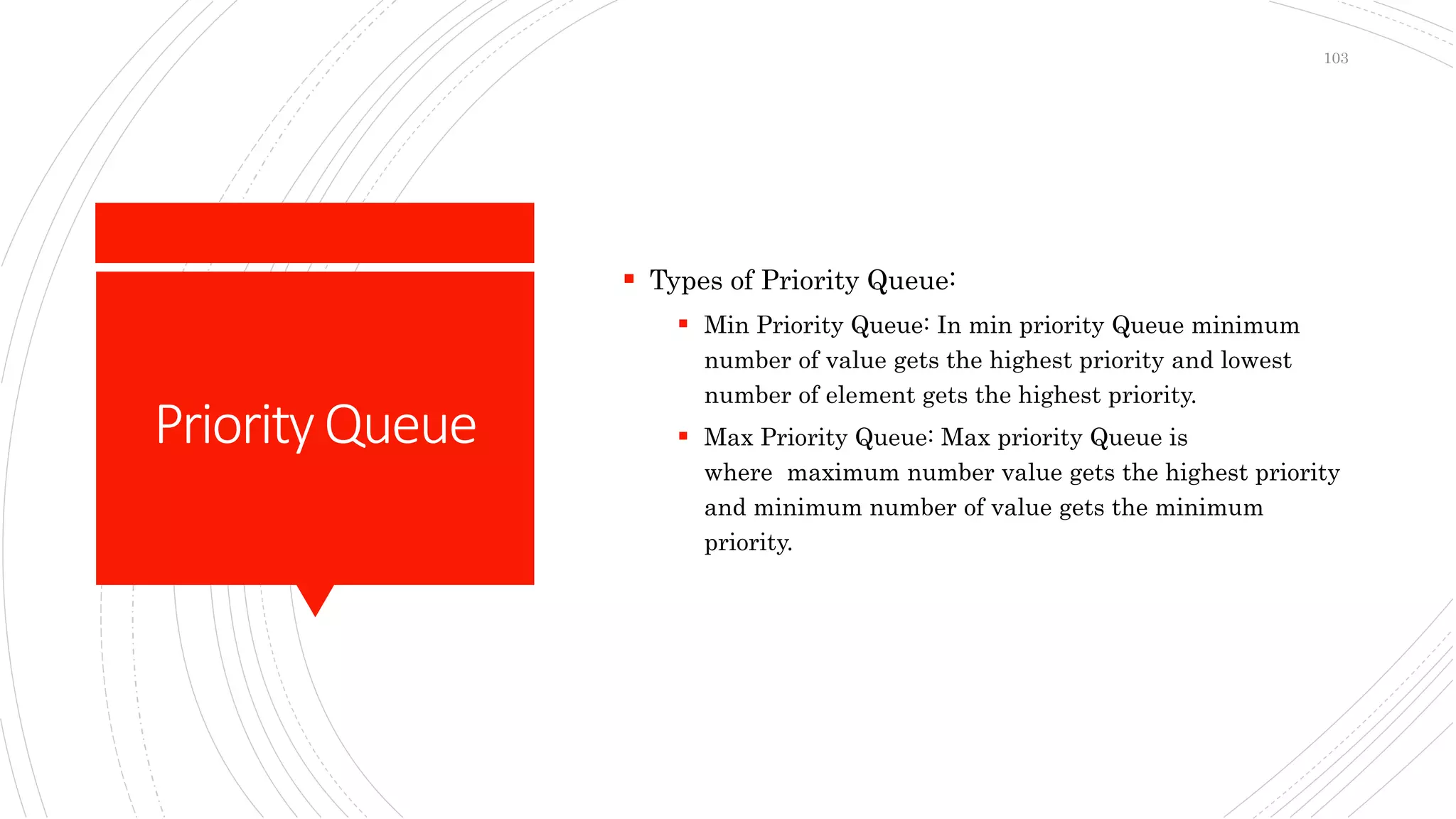
 Types of Priority Queue:
 Min Priority Queue: In min priority Queue minimum
number of value gets the highest priority and lowest
number of element gets the highest priority.
 Max Priority Queue: Max priority Queue is
where maximum number value gets the highest priority
and minimum number of value gets the minimum
priority.
103
Demonstration
ofPQueue
(Dequeue)
int deQueue() {
….....
int i, max = 0;
// find the maximum priority
for (i = 1; i < n; i++) {
if (items[max] < items[i]) {
max = i;
}
}
element = items[max]; ….....
queue[max] = queue[rear - 1];
rear = rear - 1;
104
Deque
 Types of Deque
 Input Restricted Deque: In this deque, input is restricted
at a single end but allows deletion at both the ends.
 Output Restricted Deque: In this deque, output is
restricted at a single end but allows insertion at both the
ends.
105
Demonstration
ofDeque
(State)
 boolean isFull() {
 return ((front == 0 && rear == size - 1)
|| front == rear + 1);
 }

 boolean isEmpty() {
 return (front == -1);
 }
106
Demonstration
ofDeque
(EnqueueFront)
void insertfront(int key) {
if (isFull()) {
System.out.println("Overflow");
return;
}
if (front == -1) {
front = 0;
rear = 0;
}
else if (front == 0)
front = size - 1;
else
front = front - 1;
arr[front] = key;
}
107
Demonstration
ofDeque
(EnqueueRear)
void insertrear(int key) {
if (isFull()) {
System.out.println(" Overflow ");
return;
}
if (front == -1) {
front = 0;
rear = 0;
}
else if (rear == size - 1)
rear = 0;
else
rear = rear + 1;
arr[rear] = key;
}
108
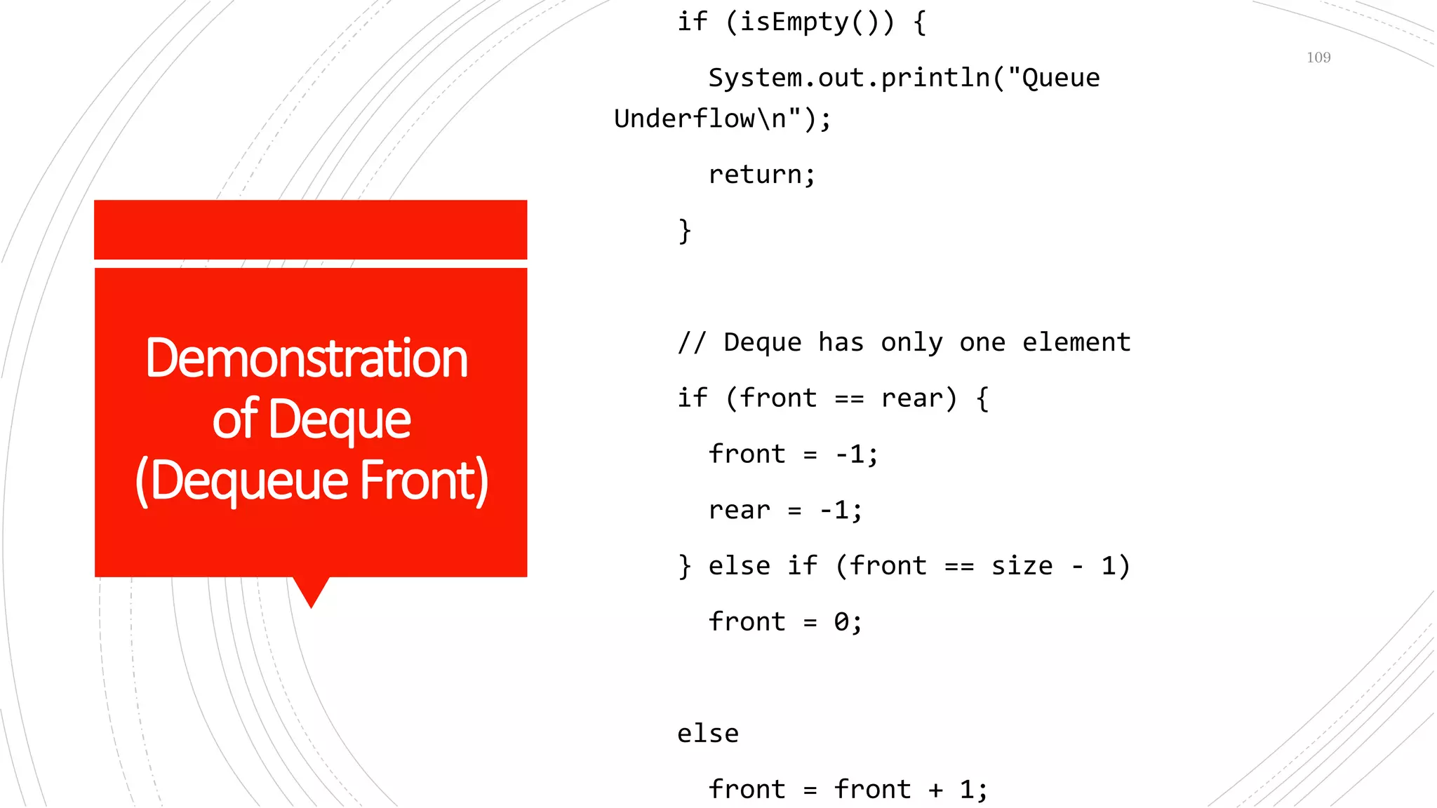
Demonstration
ofDeque
(DequeueFront)
if (isEmpty()) {
System.out.println("Queue
Underflown");
return;
}
// Deque has only one element
if (front == rear) {
front = -1;
rear = -1;
} else if (front == size - 1)
front = 0;
else
front = front + 1;
109
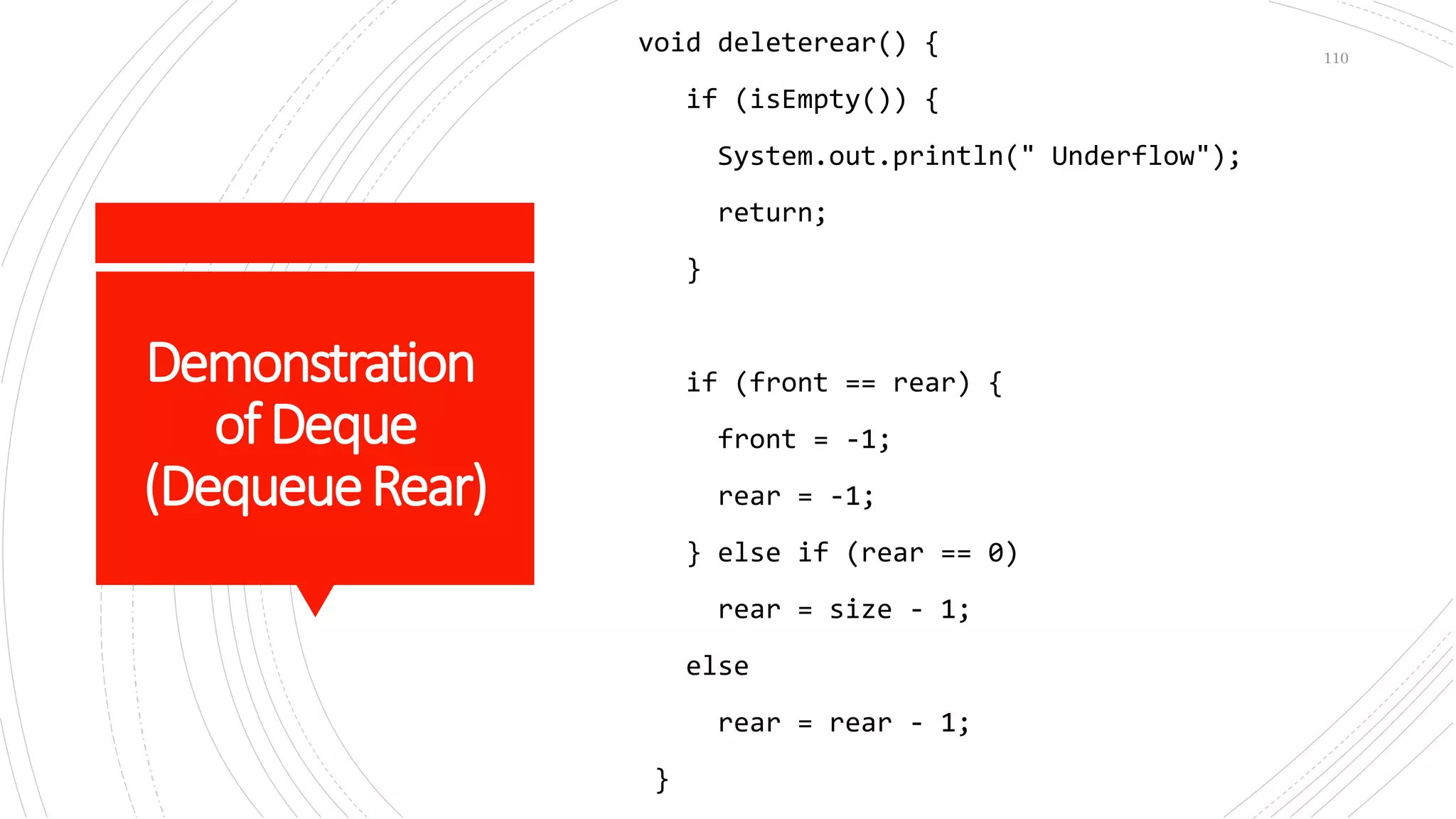
Demonstration
ofDeque
(DequeueRear)
void deleterear() {
if (isEmpty()) {
System.out.println(" Underflow");
return;
}
if (front == rear) {
front = -1;
rear = -1;
} else if (rear == 0)
rear = size - 1;
else
rear = rear - 1;
}
110
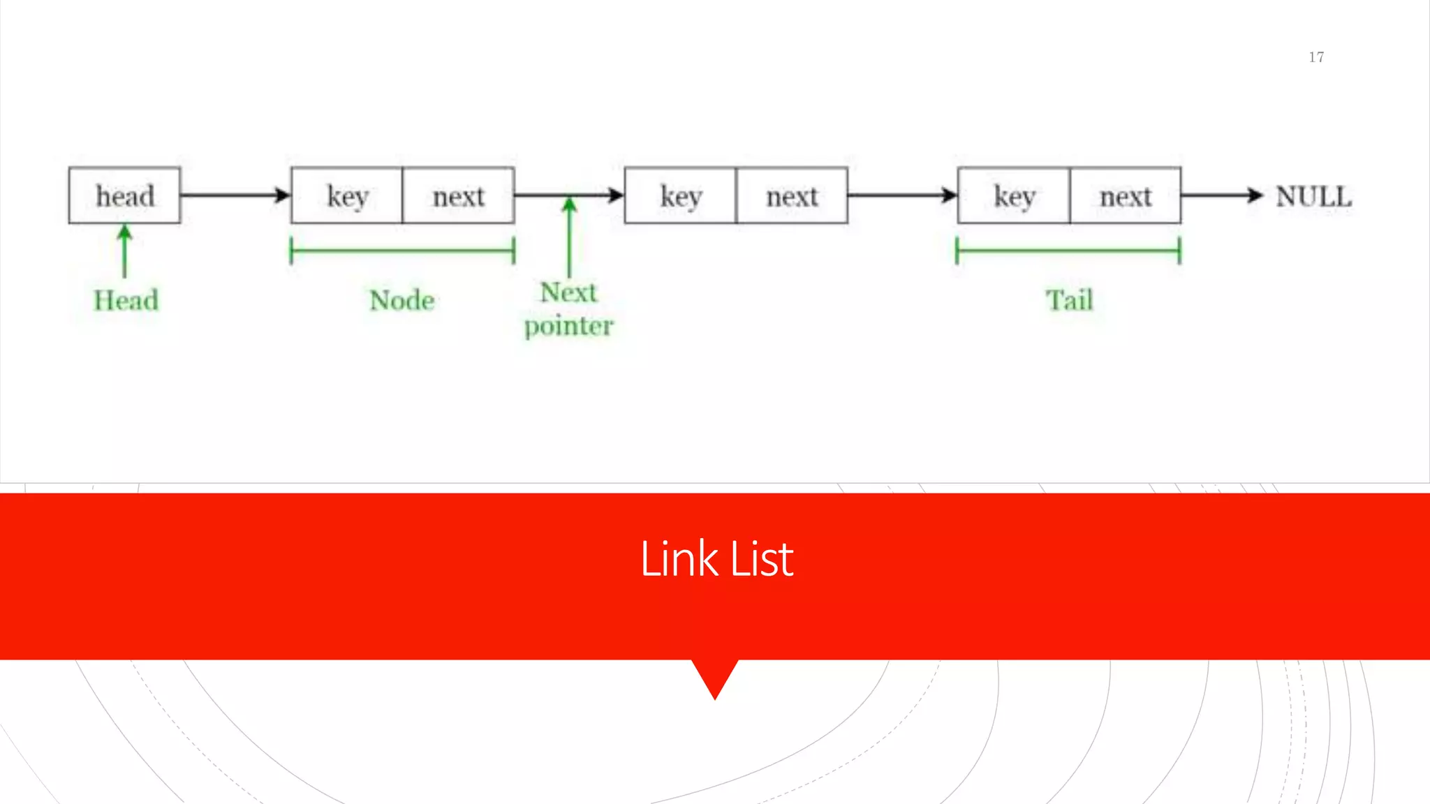
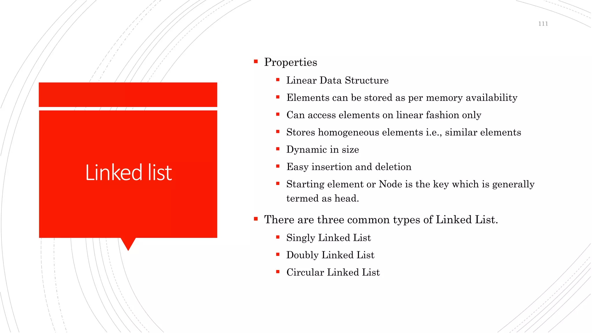
Linkedlist
 Properties
 Linear Data Structure
 Elements can be stored as per memory availability
 Can access elements on linear fashion only
 Stores homogeneous elements i.e., similar elements
 Dynamic in size
 Easy insertion and deletion
 Starting element or Node is the key which is generally
termed as head.
 There are three common types of Linked List.
 Singly Linked List
 Doubly Linked List
 Circular Linked List
111
LinkedList
 Advantages
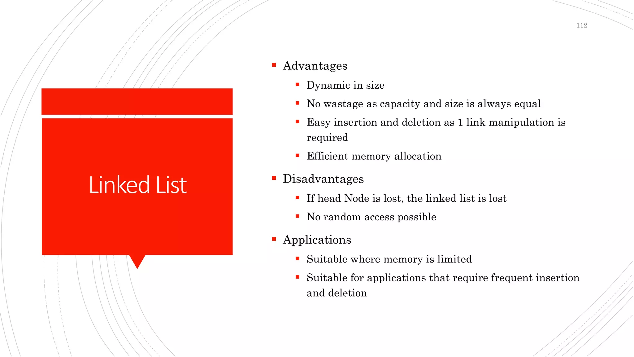
 Dynamic in size
 No wastage as capacity and size is always equal
 Easy insertion and deletion as 1 link manipulation is
required
 Efficient memory allocation
 Disadvantages
 If head Node is lost, the linked list is lost
 No random access possible
 Applications
 Suitable where memory is limited
 Suitable for applications that require frequent insertion
and deletion
112
Demonstration
ofLinked
List(Create)
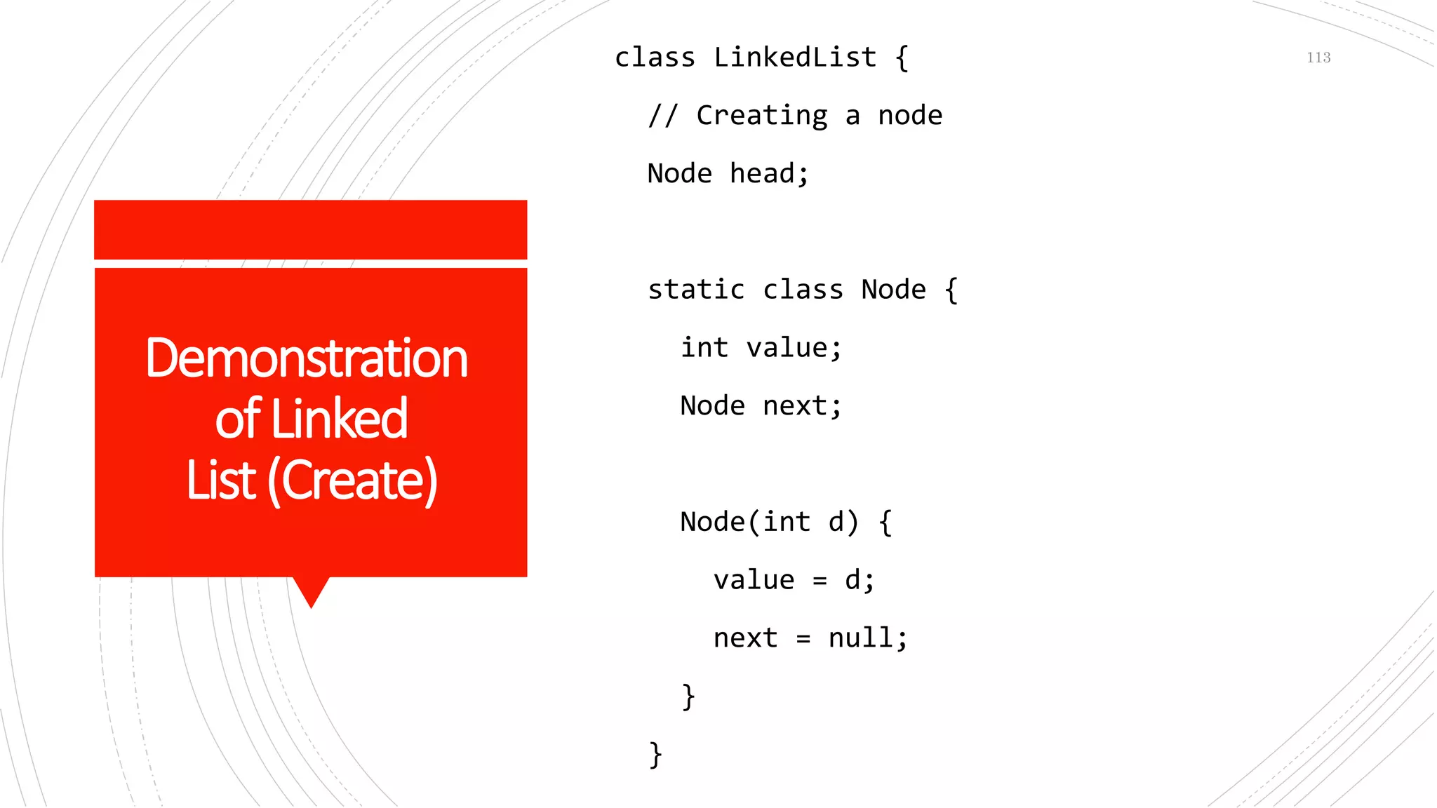
class LinkedList {
// Creating a node
Node head;
static class Node {
int value;
Node next;
Node(int d) {
value = d;
next = null;
}
}
113
Demonstrationof
LinkedList(Main)
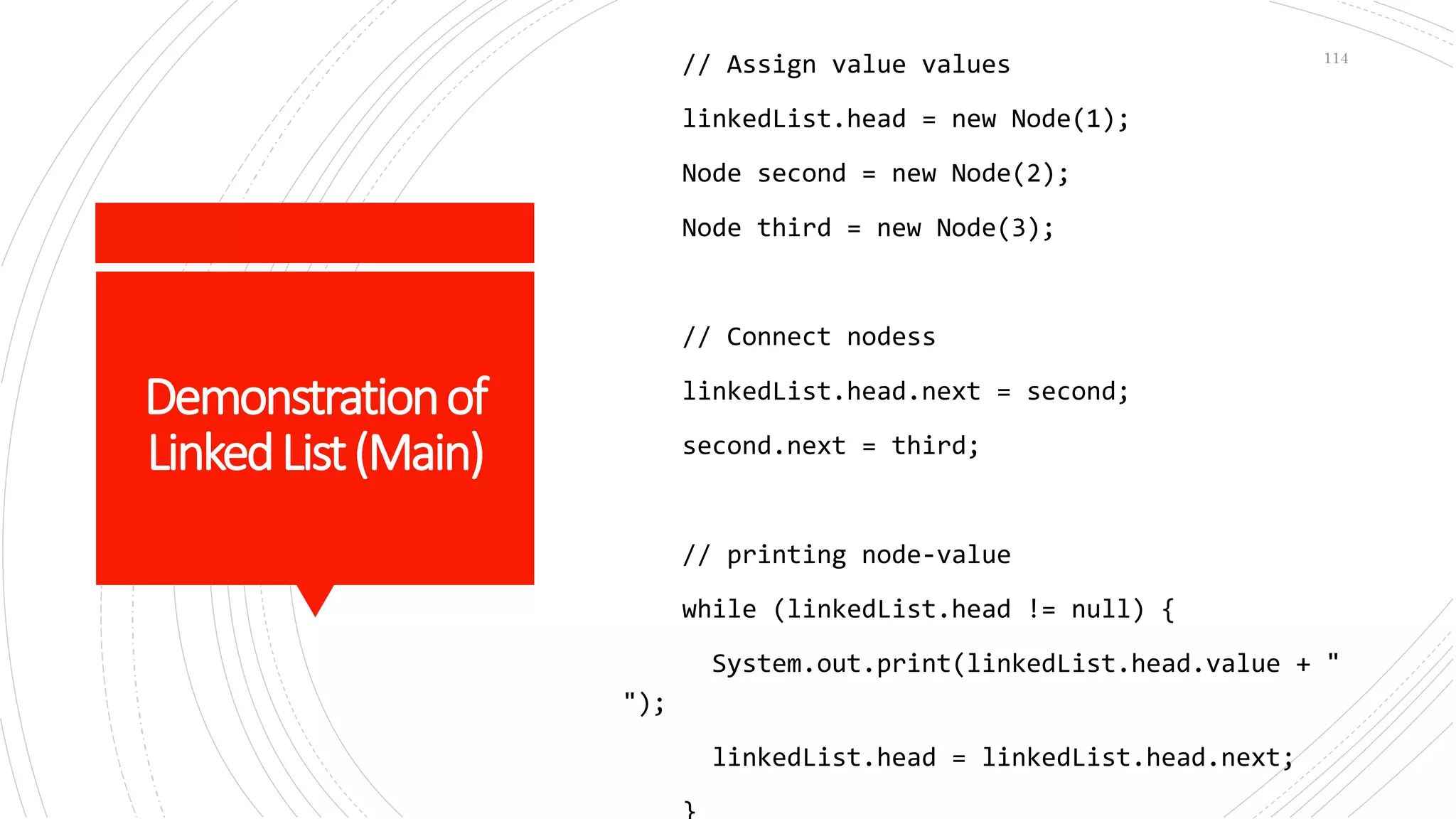
// Assign value values
linkedList.head = new Node(1);
Node second = new Node(2);
Node third = new Node(3);
// Connect nodess
linkedList.head.next = second;
second.next = third;
// printing node-value
while (linkedList.head != null) {
System.out.print(linkedList.head.value + "
");
linkedList.head = linkedList.head.next;
114
Demonstrationof
LinkedList
(InsertBeginning)
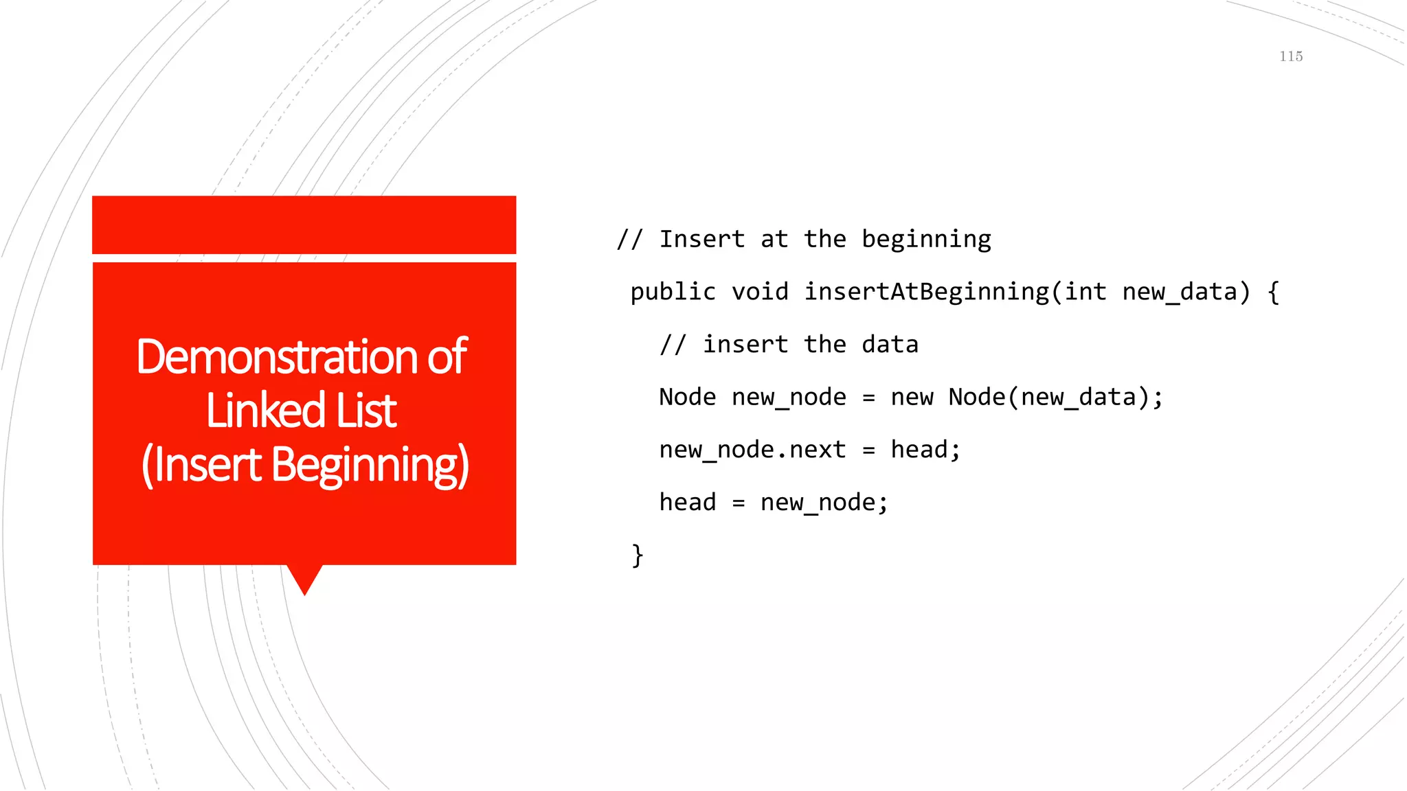
// Insert at the beginning
public void insertAtBeginning(int new_data) {
// insert the data
Node new_node = new Node(new_data);
new_node.next = head;
head = new_node;
}
115
Demonstration
ofLinkedList
(InsertEnd)
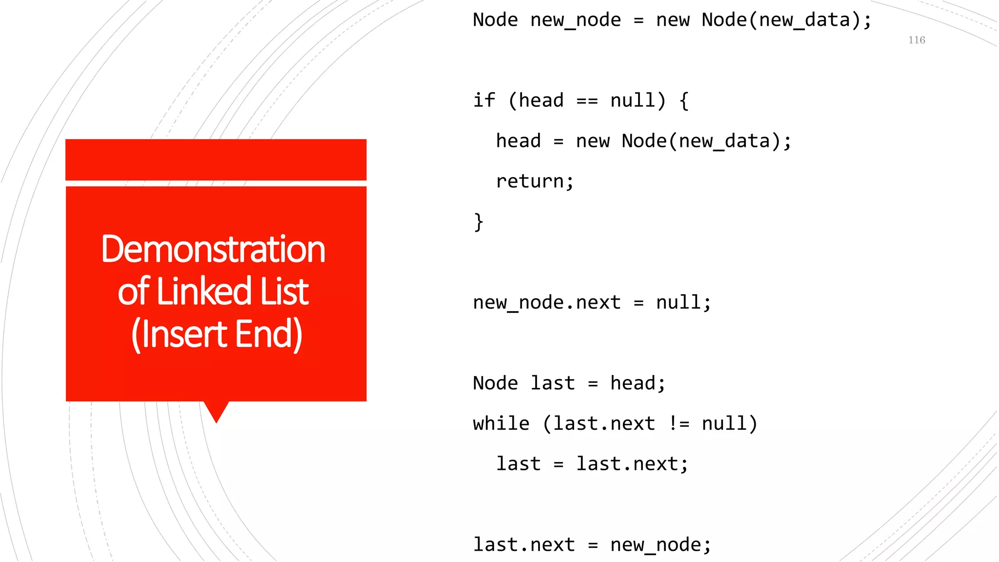
Node new_node = new Node(new_data);
if (head == null) {
head = new Node(new_data);
return;
}
new_node.next = null;
Node last = head;
while (last.next != null)
last = last.next;
last.next = new_node;
116
Demonstrationof
LinkedList
(InsertAnypoint)
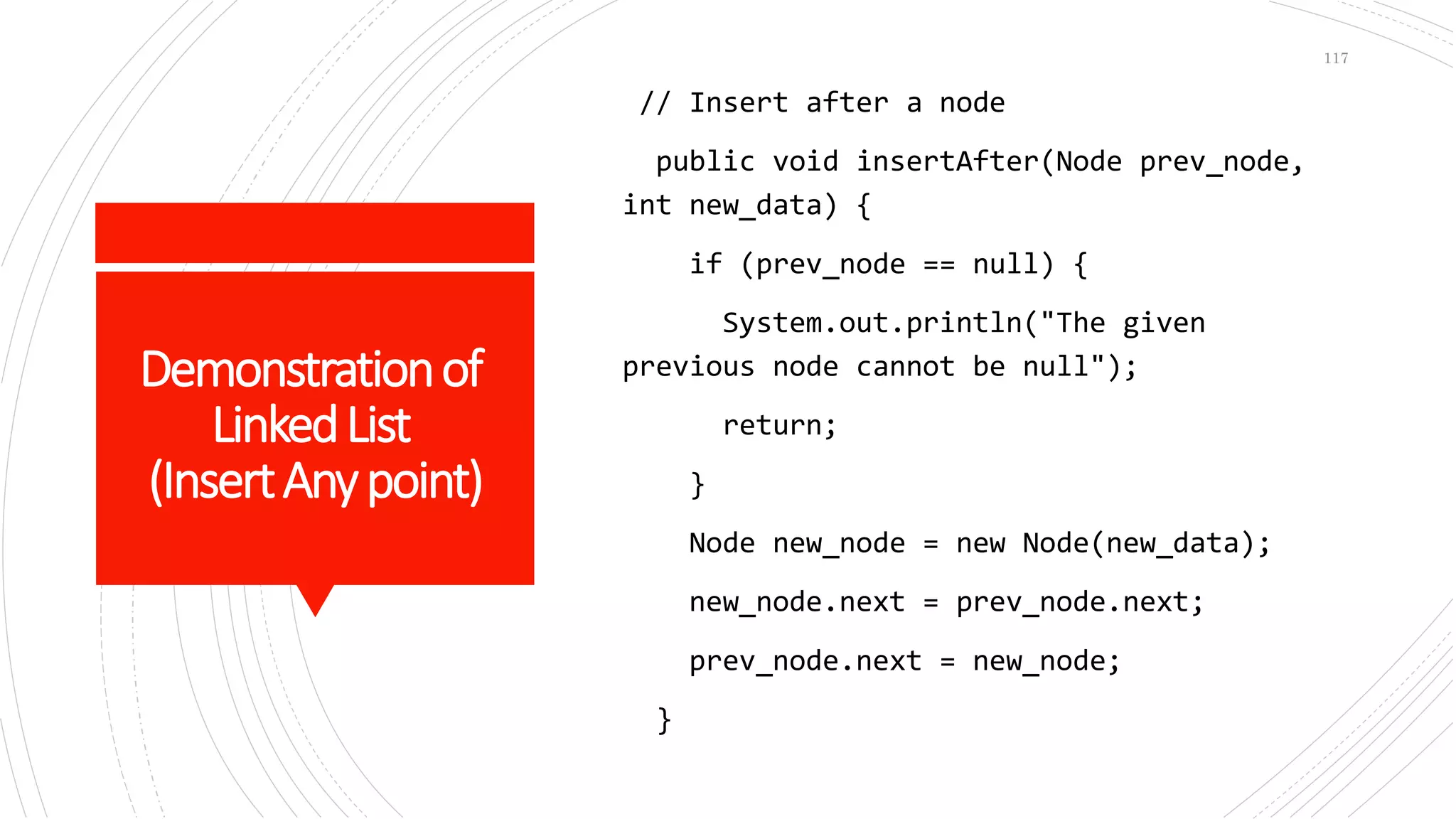
// Insert after a node
public void insertAfter(Node prev_node,
int new_data) {
if (prev_node == null) {
System.out.println("The given
previous node cannot be null");
return;
}
Node new_node = new Node(new_data);
new_node.next = prev_node.next;
prev_node.next = new_node;
}
117
Demonstration
ofLinkedList
(Delete)
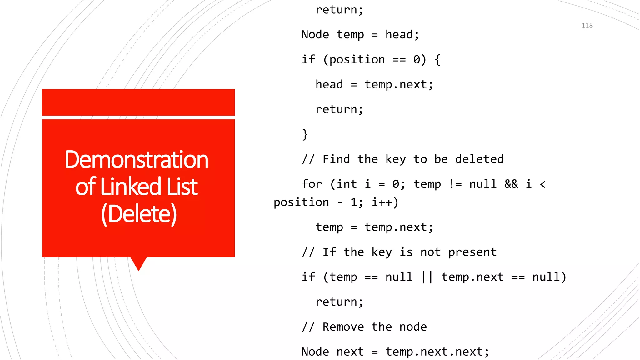
return;
Node temp = head;
if (position == 0) {
head = temp.next;
return;
}
// Find the key to be deleted
for (int i = 0; temp != null && i <
position - 1; i++)
temp = temp.next;
// If the key is not present
if (temp == null || temp.next == null)
return;
// Remove the node
Node next = temp.next.next;
118
Demonstration
ofLinkedList
(Display)
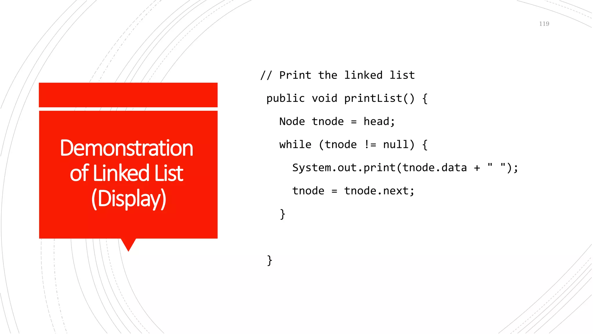
// Print the linked list
public void printList() {
Node tnode = head;
while (tnode != null) {
System.out.print(tnode.data + " ");
tnode = tnode.next;
}
}
119
Demonstration
ofDoublyLinked
List(Create)
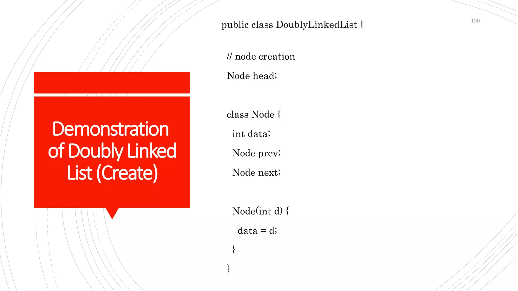
public class DoublyLinkedList {
// node creation
Node head;
class Node {
int data;
Node prev;
Node next;
Node(int d) {
data = d;
}
}
120
Demonstrationof
DoublyLinkedList
(Main)
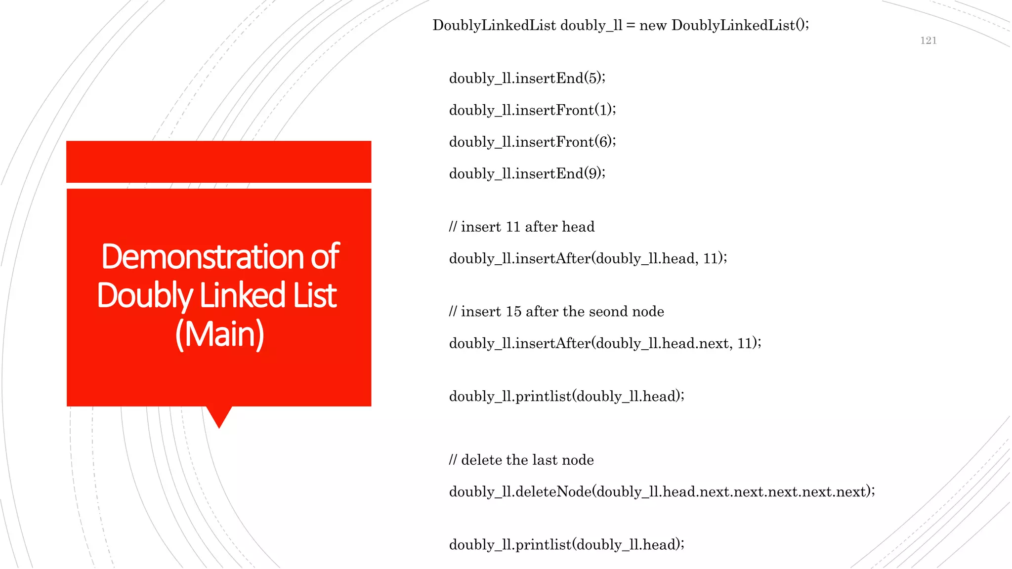
DoublyLinkedList doubly_ll = new DoublyLinkedList();
doubly_ll.insertEnd(5);
doubly_ll.insertFront(1);
doubly_ll.insertFront(6);
doubly_ll.insertEnd(9);
// insert 11 after head
doubly_ll.insertAfter(doubly_ll.head, 11);
// insert 15 after the seond node
doubly_ll.insertAfter(doubly_ll.head.next, 11);
doubly_ll.printlist(doubly_ll.head);
// delete the last node
doubly_ll.deleteNode(doubly_ll.head.next.next.next.next.next);
doubly_ll.printlist(doubly_ll.head);
121
Demonstrationof
DoubleLinkedList
(InsertBeginning)
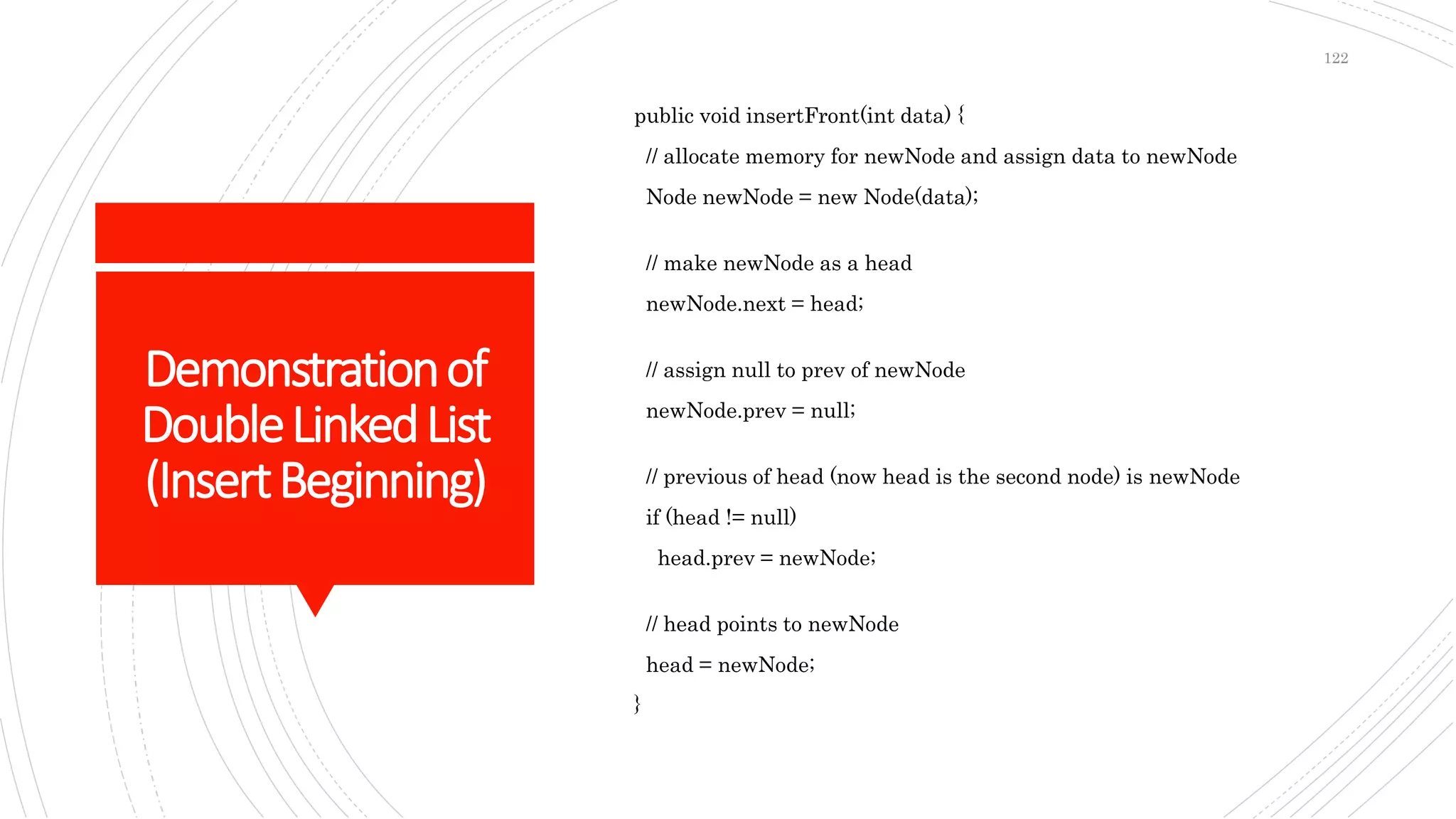
public void insertFront(int data) {
// allocate memory for newNode and assign data to newNode
Node newNode = new Node(data);
// make newNode as a head
newNode.next = head;
// assign null to prev of newNode
newNode.prev = null;
// previous of head (now head is the second node) is newNode
if (head != null)
head.prev = newNode;
// head points to newNode
head = newNode;
}
122
Demonstrationof
DoublyLinkedList
(InsertEnd)
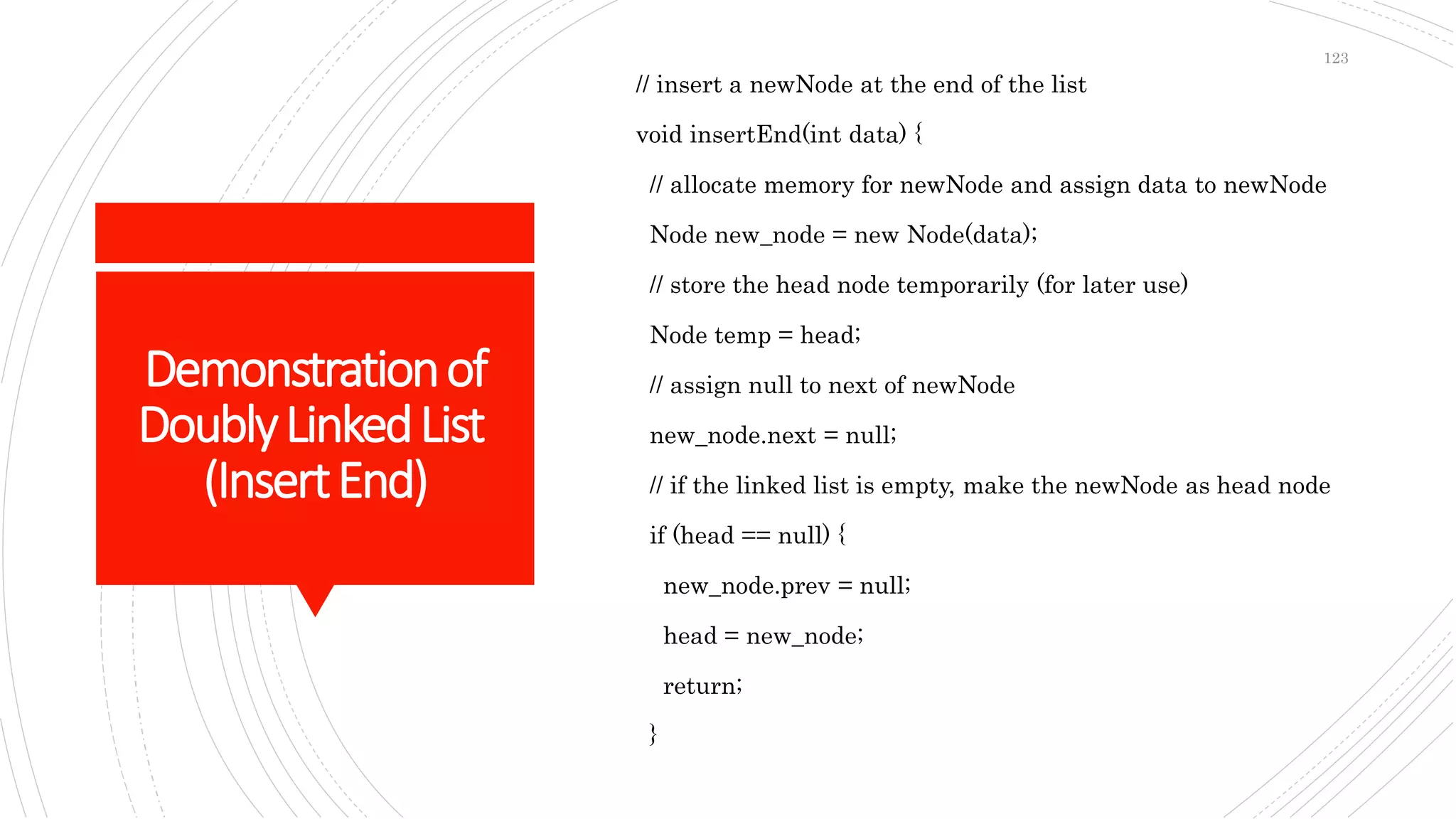
// insert a newNode at the end of the list
void insertEnd(int data) {
// allocate memory for newNode and assign data to newNode
Node new_node = new Node(data);
// store the head node temporarily (for later use)
Node temp = head;
// assign null to next of newNode
new_node.next = null;
// if the linked list is empty, make the newNode as head node
if (head == null) {
new_node.prev = null;
head = new_node;
return;
}
123
Demonstrationof
DoubleLinked
List
(AnyPoint)
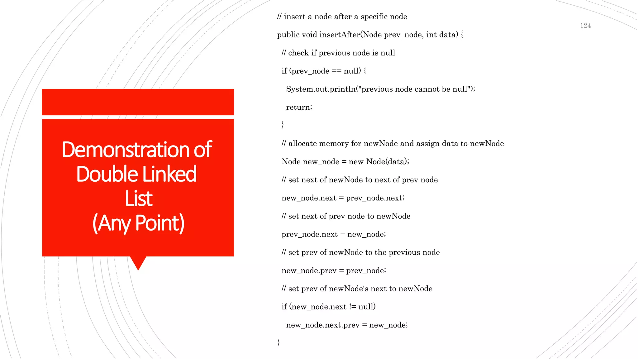
// insert a node after a specific node
public void insertAfter(Node prev_node, int data) {
// check if previous node is null
if (prev_node == null) {
System.out.println("previous node cannot be null");
return;
}
// allocate memory for newNode and assign data to newNode
Node new_node = new Node(data);
// set next of newNode to next of prev node
new_node.next = prev_node.next;
// set next of prev node to newNode
prev_node.next = new_node;
// set prev of newNode to the previous node
new_node.prev = prev_node;
// set prev of newNode's next to newNode
if (new_node.next != null)
new_node.next.prev = new_node;
}
124
"The only way to learn a new
programming language is by
writing programs in it."
Dennis Ritchie
125
CircularLinkList
 Connect Last to Head by storing value of Head in
Last's node next
126
Sortingand
Searching
 Storing and retrieving information is one of the most
common application of computers now-a-days.
 According to time the amount of data and information
stored and accessed via computer has turned to
huge databases.
 So many techniques and algorithms have been
developed to efficiently maintain and process
information in databases.
 The processes of looking up a particular data record in
the database is called searching.
 The process of ordering the records in a database is
called Sorting.
 Sorting and searching together constitute a major area
of study in computational methods.
127
Search
 Searching is the process of finding a particular item in
a collection of items.
 A search typically answers whether the item is present
in the collection or not.
 When the key field of a target item is found, a pointer
to the target item is returned.
 The pointer may be an address, an index into a vector
or array, or some other indication of where to find the
target.
 If a matching key field isn’t found, the user is
informed.
128
Common
Searching
Algorithms
 Linear search
 Binary search
129
LinearSearch
Step 1: Set i to 1
Step 2: if i > n then go to step 7
Step 3: if A[i] = x then go to step 6
Step 4: Set i to i + 1
Step 5: Go to Step 2
Step 6: Print Element x Found at index i and go
to step 8
Step 7: Print element not found
130
JavaCode
class LinearSearch {
public static int linearSearch(int array[], int x) {
int n = array.length;
// Going through array sequencially
for (int i = 0; i < n; i++) {
if (array[i] == x)
return i;
}
return -1;
}
public static void main(String args[]) {
int array[] = { 2, 4, 0, 1, 9 };
int x = 1;
int result = linearSearch(array, x);
if (result == -1)
System.out.print("Element not found");
else
System.out.print("Element found at index: " + result);
}
}
131
BinarySearch
Step 1: Data list must be ordered list in ascending
order.
Step 2: Probe middle of list
Step 3: If target equals list[mid], FOUND.
Step 4: If target < list[mid], discard 1/2 of list
between list[mid] and list[last].
Step 5: If target > list[mid], discard 1/2 of list
between list[first] and list[mid].
Step 6: Continue searching the shortened list until
either the target is found, or there are no
elements to probe.
132
JavaCode
while (low <= high) {
int mid = low + (high - low) / 2;
if (array[mid] == x)
return mid;
if (array[mid] < x)
low = mid + 1;
else
high = mid - 1;
}
return -1;
}
public static void main(String args[]) {
BinarySearch ob = new BinarySearch();
int array[] = { 3, 4, 5, 6, 7, 8, 9 };
int n = array.length;
int x = 4;
int result = ob.binarySearch(array, x, 0, n - 1);
if (result == -1)
System.out.println("Not found");
else
133
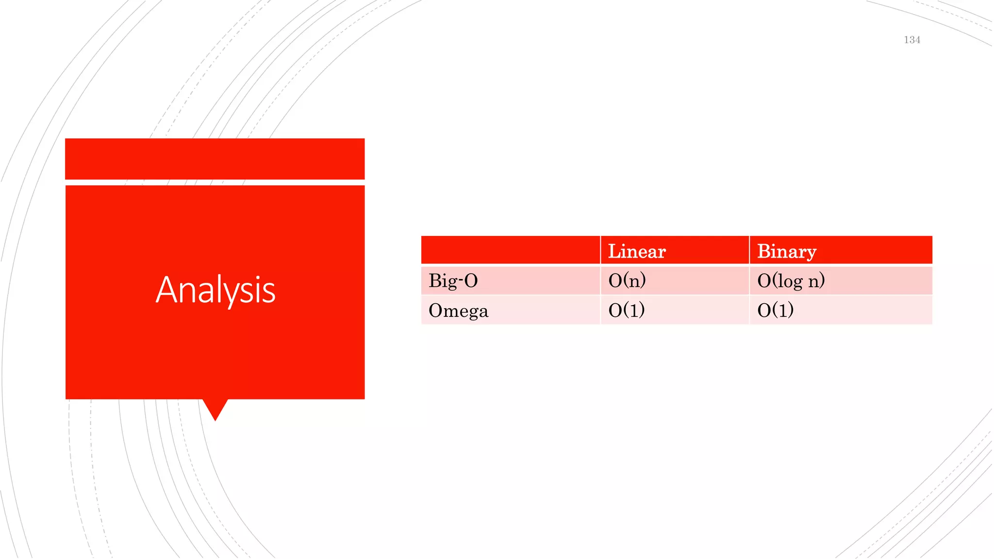
Analysis
Linear Binary
Big-O O(n) O(log n)
Omega O(1) O(1)
134
Sort
 Sorting is the process of placing elements from a
collection in order.
 For example, a list of words could be sorted
alphabetically or by length.
 Efficient sorting is important to optimize the use of
other algorithms that require sorted lists to work
correctly.
 There are two main types of Sort:
 Internal (Sort happens in primary memory)
 External (Sort happens in primary + secondary memory)
135
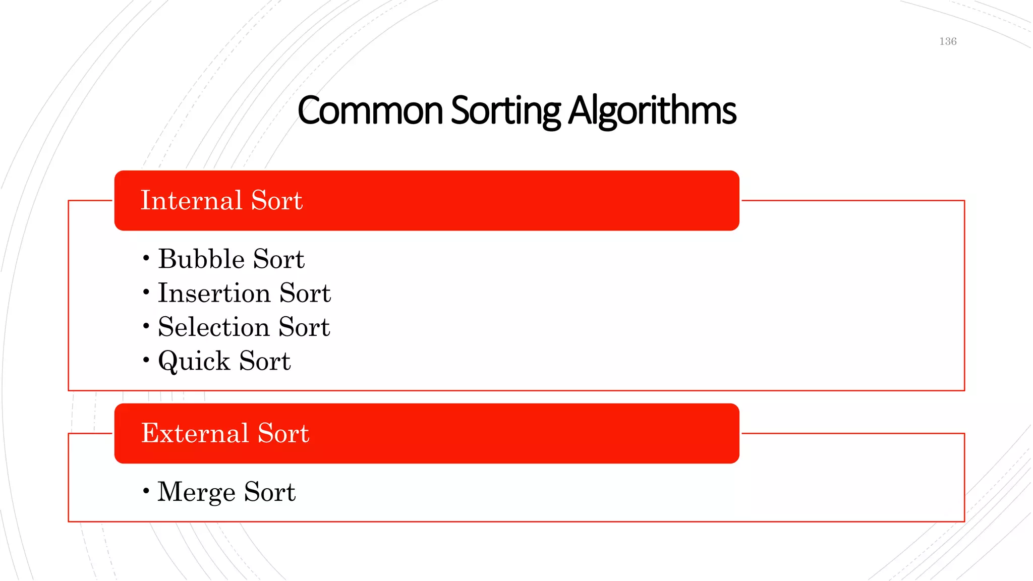
CommonSortingAlgorithms
•Bubble Sort
•Insertion Sort
•Selection Sort
•Quick Sort
Internal Sort
•Merge Sort
External Sort
136
Bubble
set swap flag to false
for j=1 to i {
if list[j-1] > list[j]
swap list[j-1] and list[j]
set swap flag to true
}
if swap flag is false, break. The list is
sorted.
137
Java Code
{
int i, j, temp;
for(i = 0; i < n; i++)
{
for(j = 0; j < n-i-1; j++)
{
if( arr[j] > arr[j+1])
{
// swap the elements
temp = arr[j];
arr[j] = arr[j+1];
arr[j+1] = temp;
}
}
138
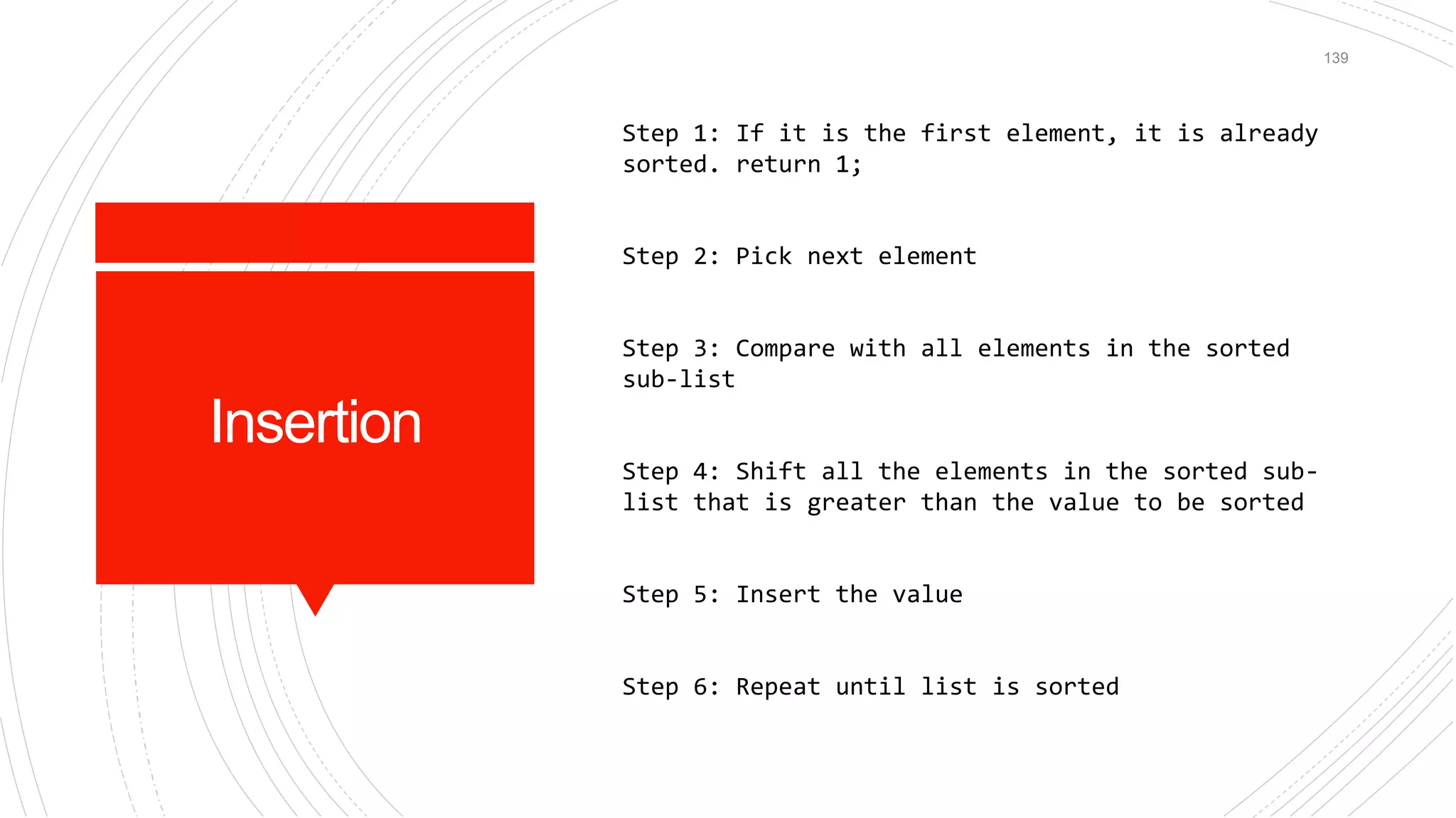
Insertion
Step 1: If it is the first element, it is already
sorted. return 1;
Step 2: Pick next element
Step 3: Compare with all elements in the sorted
sub-list
Step 4: Shift all the elements in the sorted sub-
list that is greater than the value to be sorted
Step 5: Insert the value
Step 6: Repeat until list is sorted
139
Java Code
{
int i, j, key;
for (i = 1; i < length; i++)
{
j = i;
while (j > 0 && arr[j - 1] >
arr[j])
{
key = arr[j];
arr[j] = arr[j - 1];
arr[j - 1] = key;
j--;
}
}
140
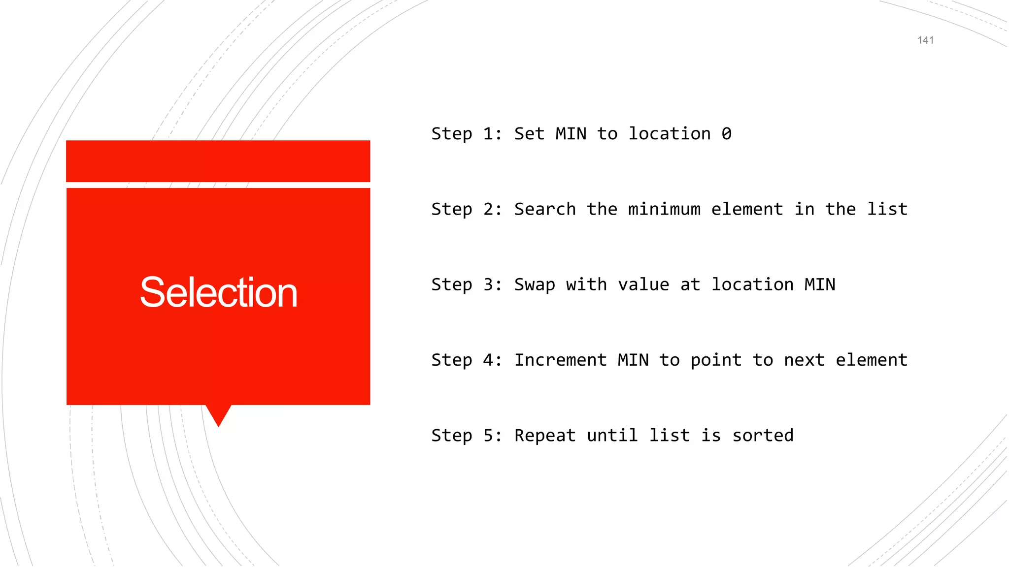
Selection
Step 1: Set MIN to location 0
Step 2: Search the minimum element in the list
Step 3: Swap with value at location MIN
Step 4: Increment MIN to point to next element
Step 5: Repeat until list is sorted
141
Java Code
int n){
int minValue = arr[startIndex];
int minIndex = startIndex;
for(int i = minIndex + 1; i < n;
i++) {
if(arr[i] < minValue) {
minIndex = i;
minValue = arr[i];
} }
return minIndex;
}
void selectionSort(int arr[], int n){
for(int i = 0; i < n; i++) {
int index = indexOfMinimum(arr, i,
n);
142
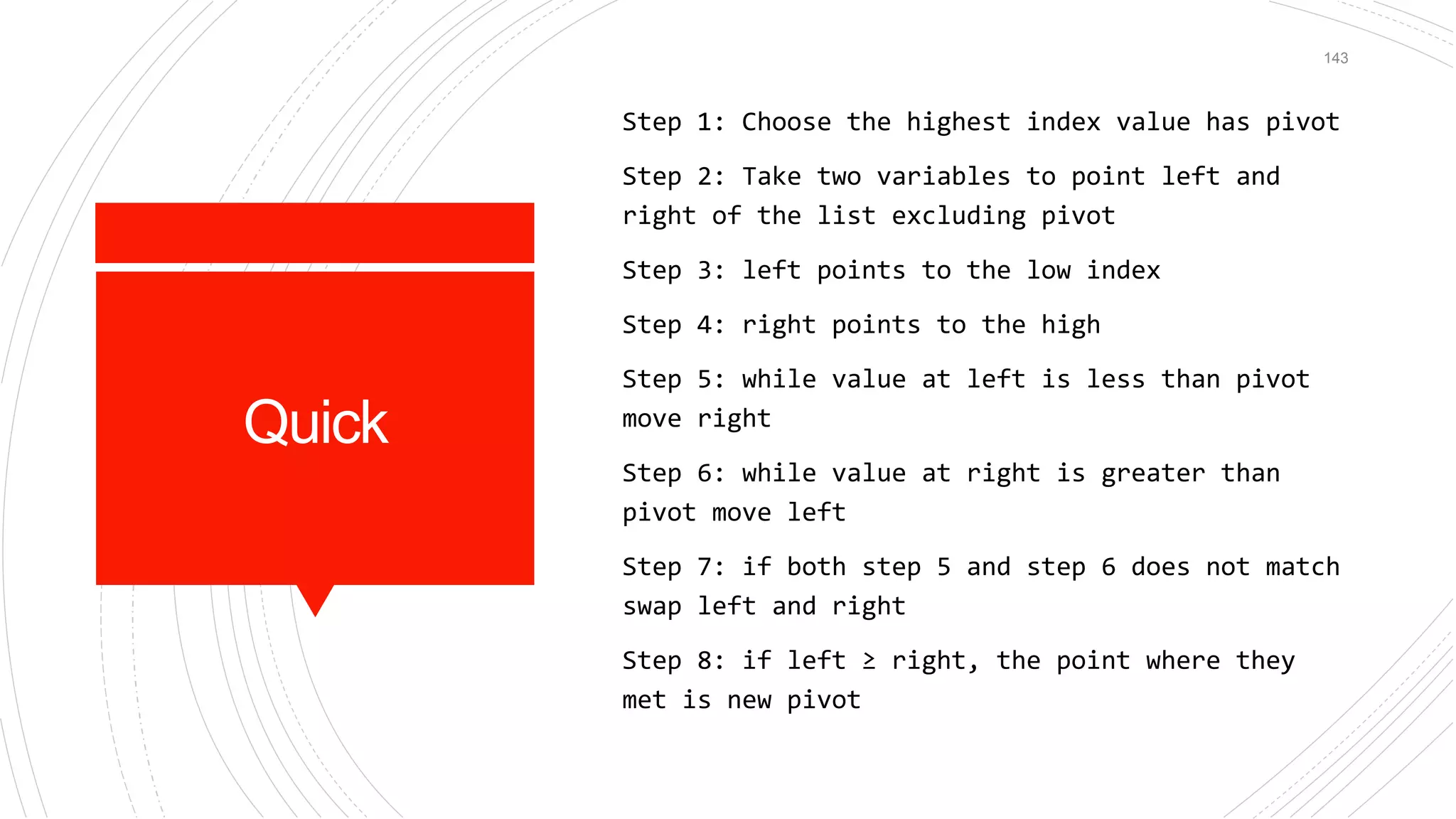
Quick
Step 1: Choose the highest index value has pivot
Step 2: Take two variables to point left and
right of the list excluding pivot
Step 3: left points to the low index
Step 4: right points to the high
Step 5: while value at left is less than pivot
move right
Step 6: while value at right is greater than
pivot move left
Step 7: if both step 5 and step 6 does not match
swap left and right
Step 8: if left ≥ right, the point where they
met is new pivot
143
Java Code
static void quickSort(int array[], int low, int high)
{
if (low < high) {
// find pivot element such that
// elements smaller than pivot are on the left
// elements greater than pivot are on the right
int pi = partition(array, low, high);
// recursive call on the left of pivot
quickSort(array, low, pi - 1);
// recursive call on the right of pivot
quickSort(array, pi + 1, high);
}
}
144
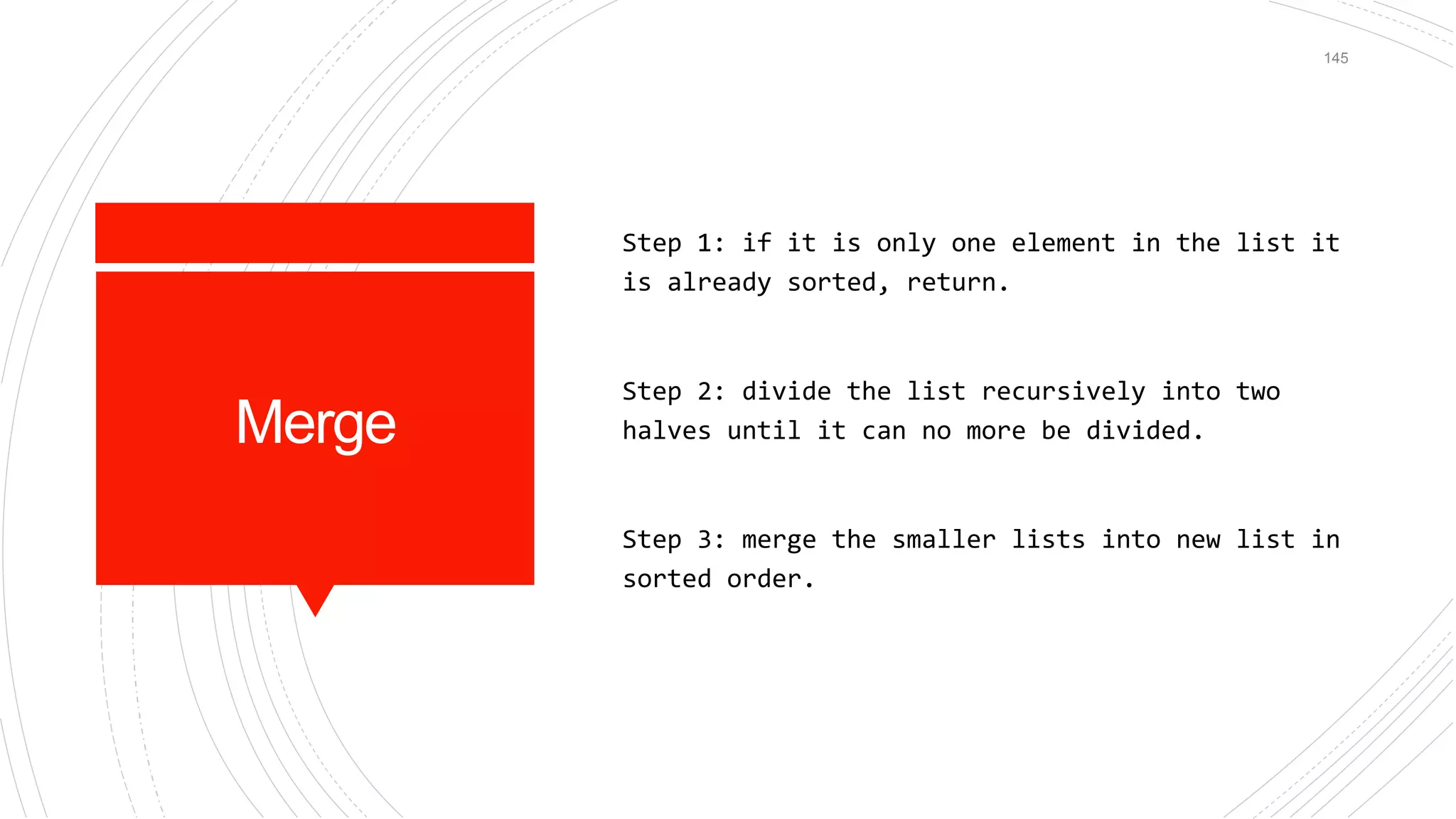
Merge
Step 1: if it is only one element in the list it
is already sorted, return.
Step 2: divide the list recursively into two
halves until it can no more be divided.
Step 3: merge the smaller lists into new list in
sorted order.
145
Java Code
void mergeSort(int arr[], int l, int r) {
if (l < r) {
// m is the point where the array is divided
into two subarrays
int m = (l + r) / 2;
mergeSort(arr, l, m);
mergeSort(arr, m + 1, r);
// Merge the sorted subarrays
merge(arr, l, m, r);
}
}
146
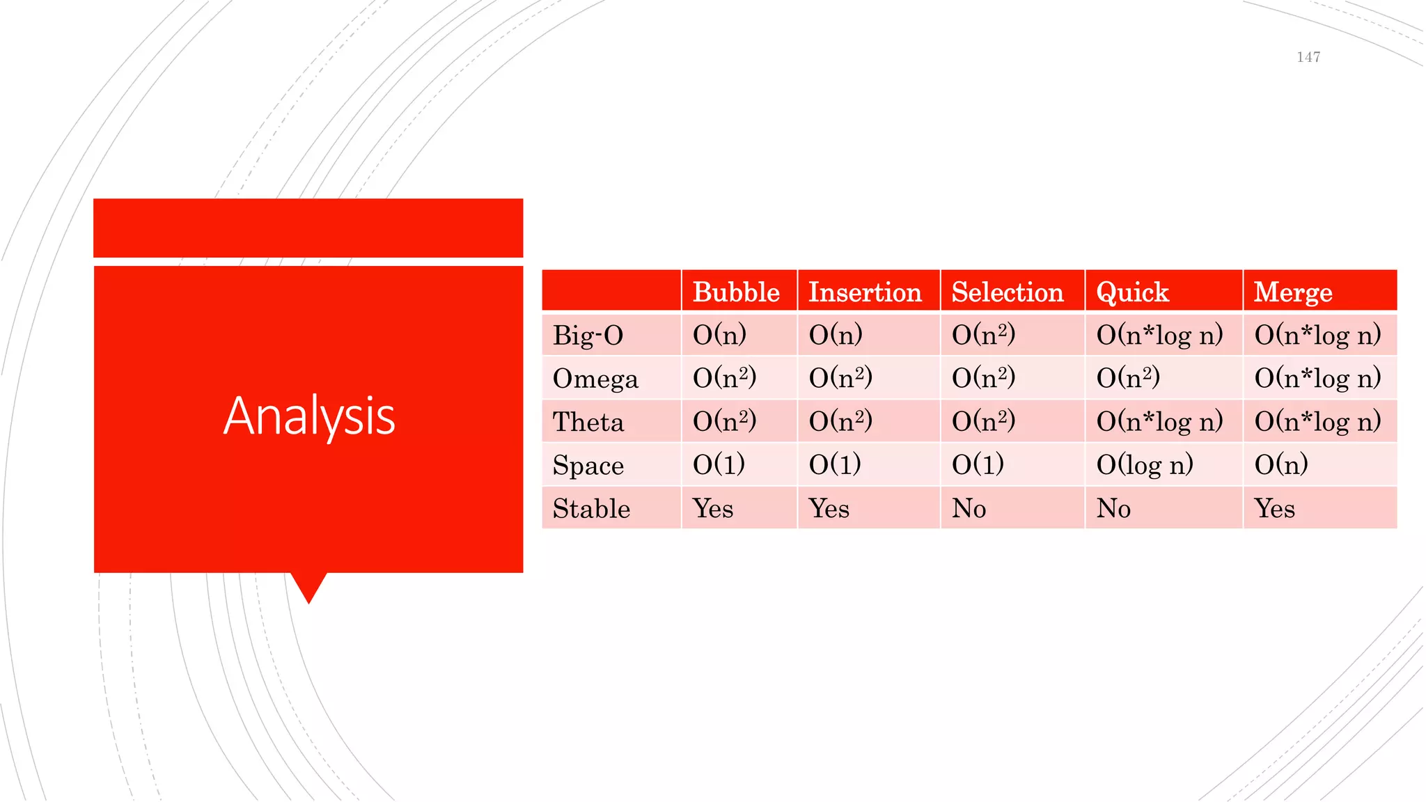
Analysis
Bubble Insertion Selection Quick Merge
Big-O O(n) O(n) O(n2) O(n*log n) O(n*log n)
Omega O(n2) O(n2) O(n2) O(n2) O(n*log n)
Theta O(n2) O(n2) O(n2) O(n*log n) O(n*log n)
Space O(1) O(1) O(1) O(log n) O(n)
Stable Yes Yes No No Yes
147
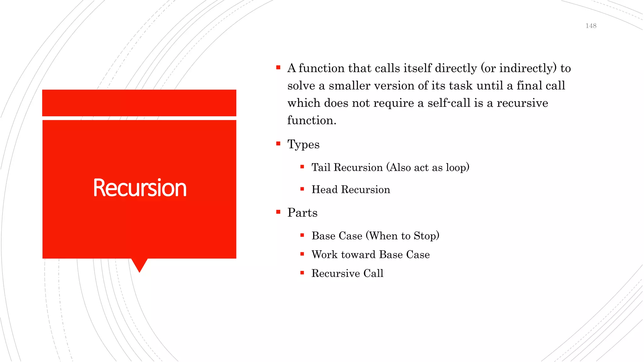
Recursion
 A function that calls itself directly (or indirectly) to
solve a smaller version of its task until a final call
which does not require a self-call is a recursive
function.
 Types
 Tail Recursion (Also act as loop)
 Head Recursion
 Parts
 Base Case (When to Stop)
 Work toward Base Case
 Recursive Call
148
149
"In some ways, programming
is like painting. You start with
a blank canvas and certain
basic raw materials. You use
a combination of science,
art, and craft to determine
what to do with them."
150
LinearSearchin
LinkedList
(Iterative)
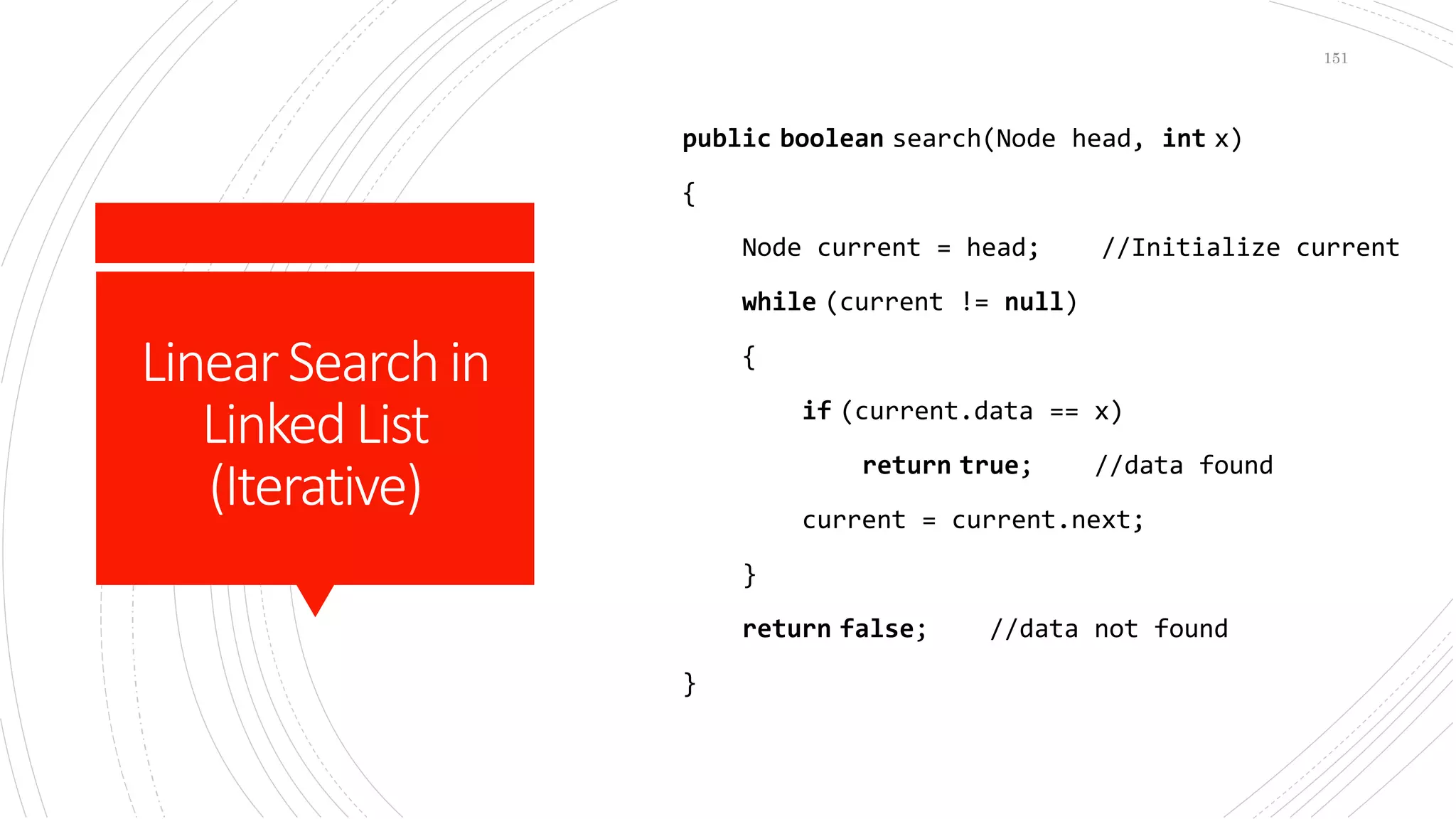
public boolean search(Node head, int x)
{
Node current = head; //Initialize current
while (current != null)
{
if (current.data == x)
return true; //data found
current = current.next;
}
return false; //data not found
}
151
LinearSearchin
LinkedList
(Recursion)
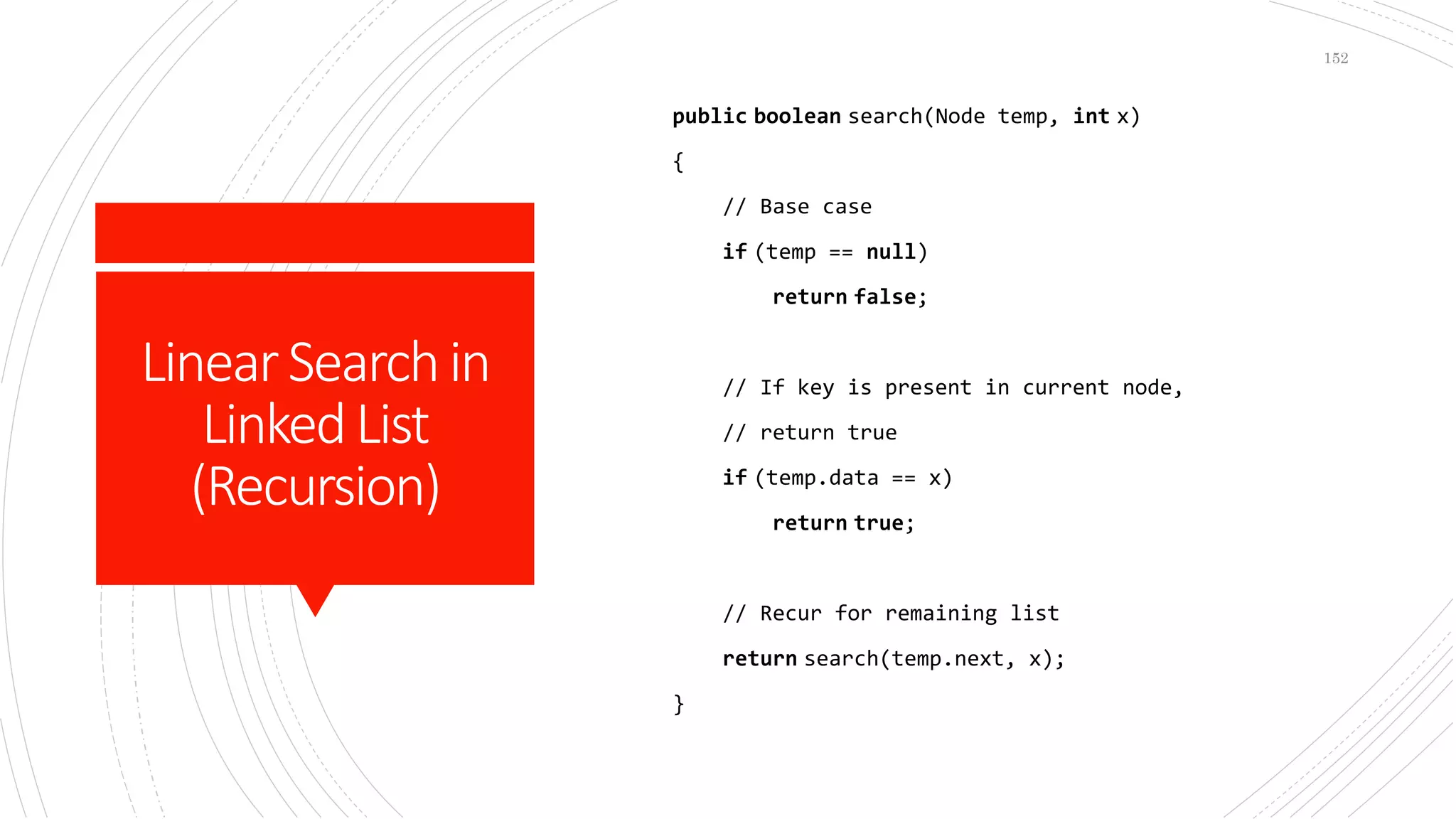
public boolean search(Node temp, int x)
{
// Base case
if (temp == null)
return false;
// If key is present in current node,
// return true
if (temp.data == x)
return true;
// Recur for remaining list
return search(temp.next, x);
}
152
Tree
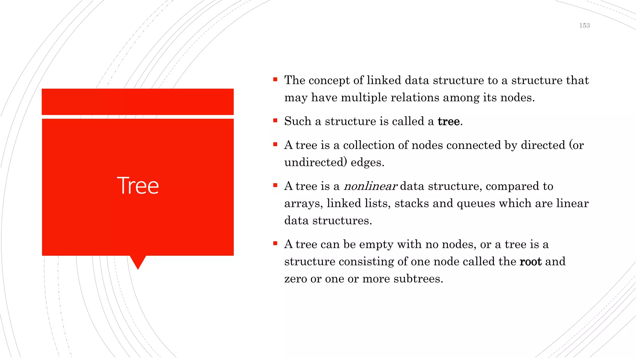
 The concept of linked data structure to a structure that
may have multiple relations among its nodes.
 Such a structure is called a tree.
 A tree is a collection of nodes connected by directed (or
undirected) edges.
 A tree is a nonlinear data structure, compared to
arrays, linked lists, stacks and queues which are linear
data structures.
 A tree can be empty with no nodes, or a tree is a
structure consisting of one node called the root and
zero or one or more subtrees.
153
Terminologies
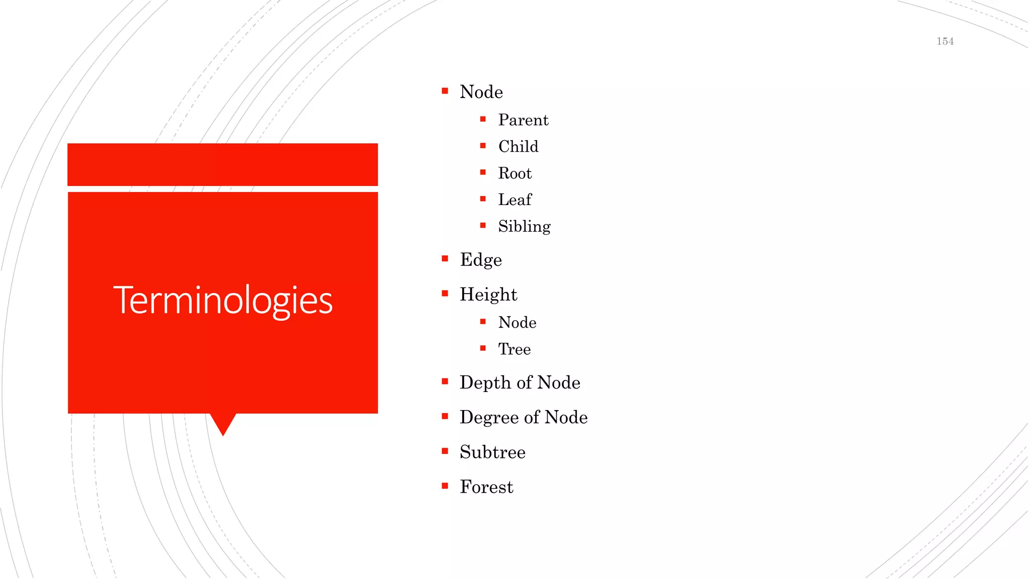
 Node
 Parent
 Child
 Root
 Leaf
 Sibling
 Edge
 Height
 Node
 Tree
 Depth of Node
 Degree of Node
 Subtree
 Forest
154
Types
 Binary Tree
 Full Binary Tree
 Perfect Binary Tree
 Balanced Binary Tree
 Binary Search Tree
 AVL Tree
 General Tree
155
Operations
 Insertion
 Deletion
 Search
 Traversal
 Breadth First
 Depth First
156
Depth
First Traversal
 In-Order
 Step 1- Recursively traverse the left subtree
 Step 2- Visit root node
 Step 3- Recursively traverse right subtree
 Pre-order
 Step 1- Visit root node
 Step 2- Recursively traverse the left subtree
 Step 3- Recursively traverse right subtree
 Post-order
 Step 1- Recursively traverse the left subtree
 Step 2- Recursively traverse right subtree
 Step 3- Visit root node
157
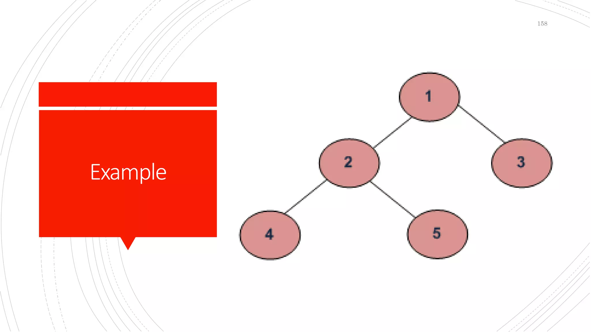
Example
158
In-Order
void printInorder(Node node)
{
if (node == null)
return;
/* first recur on left child */
printInorder(node.left);
/* then print the data of node */
System.out.print(node.key + " ");
/* now recur on right child */
printInorder(node.right);
}
159
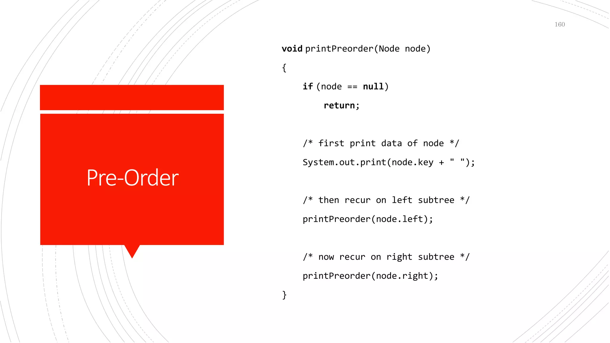
Pre-Order
void printPreorder(Node node)
{
if (node == null)
return;
/* first print data of node */
System.out.print(node.key + " ");
/* then recur on left subtree */
printPreorder(node.left);
/* now recur on right subtree */
printPreorder(node.right);
}
160
Post-Order
void printPostorder(Node node)
{
if (node == null)
return;
// first recur on left subtree
printPostorder(node.left);
// then recur on right subtree
printPostorder(node.right);
// now deal with the node
System.out.print(node.key + " ");
}
161
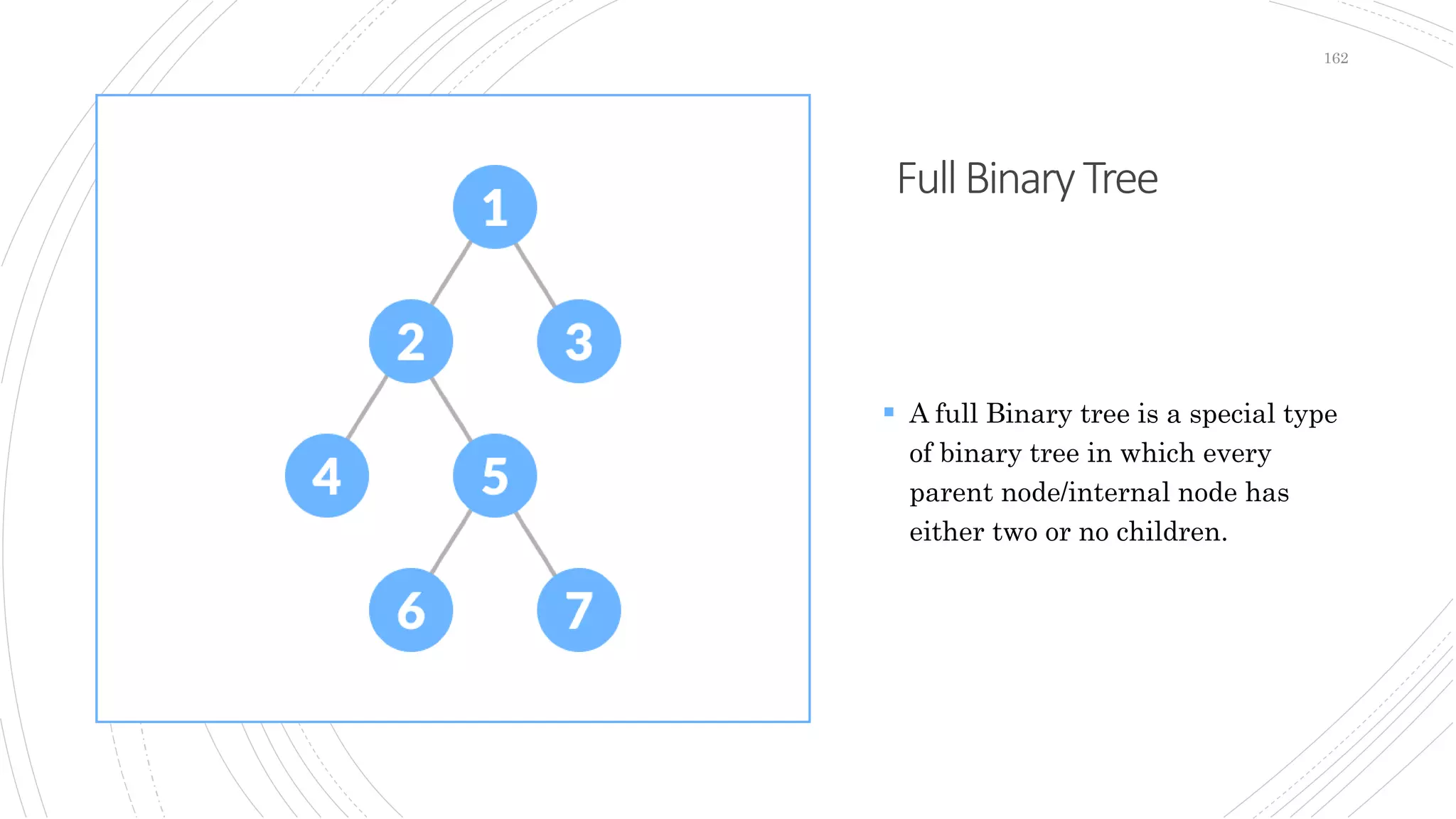
FullBinaryTree
162
 A full Binary tree is a special type
of binary tree in which every
parent node/internal node has
either two or no children.
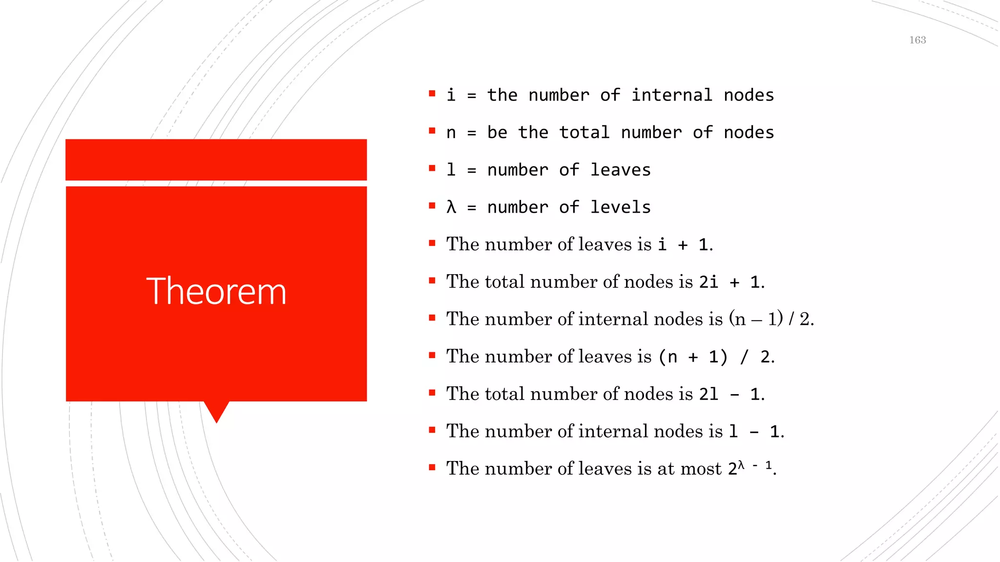
Theorem
 i = the number of internal nodes
 n = be the total number of nodes
 l = number of leaves
 λ = number of levels
 The number of leaves is i + 1.
 The total number of nodes is 2i + 1.
 The number of internal nodes is (n – 1) / 2.
 The number of leaves is (n + 1) / 2.
 The total number of nodes is 2l – 1.
 The number of internal nodes is l – 1.
 The number of leaves is at most 2λ - 1.
163
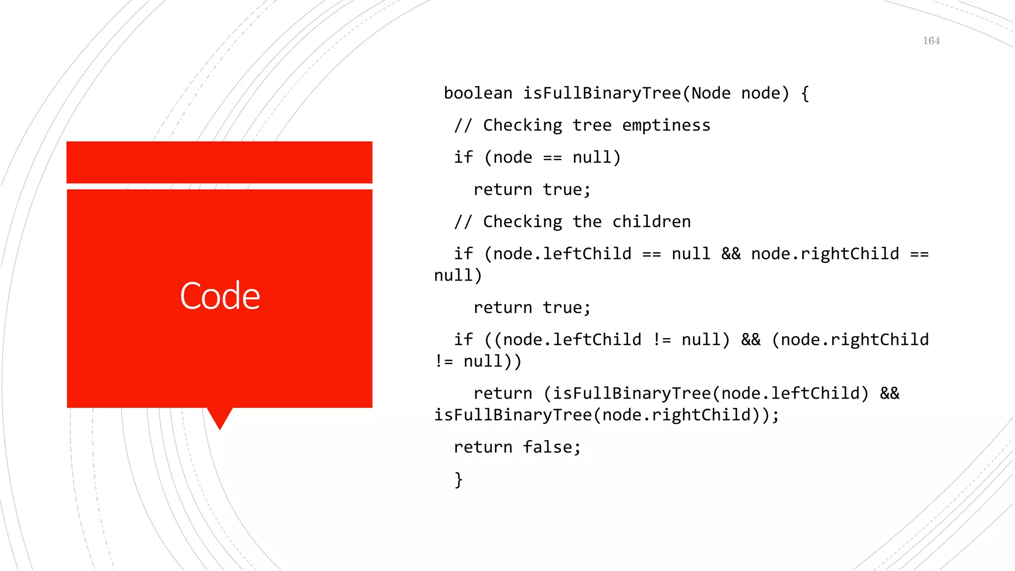
Code
boolean isFullBinaryTree(Node node) {
// Checking tree emptiness
if (node == null)
return true;
// Checking the children
if (node.leftChild == null && node.rightChild ==
null)
return true;
if ((node.leftChild != null) && (node.rightChild
!= null))
return (isFullBinaryTree(node.leftChild) &&
isFullBinaryTree(node.rightChild));
return false;
}
164
PerfectBinaryTree
165
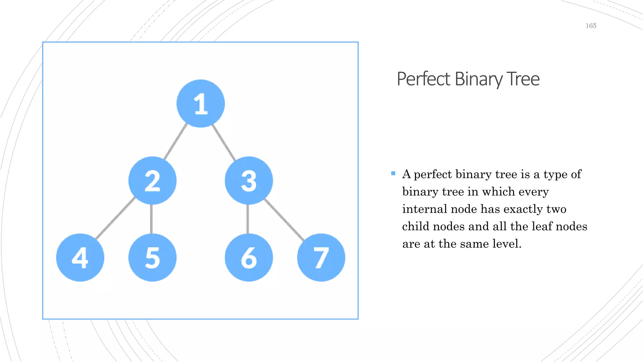
 A perfect binary tree is a type of
binary tree in which every
internal node has exactly two
child nodes and all the leaf nodes
are at the same level.
Theorem
 A perfect binary tree of height h has 2h + 1 – 1 node.
 A perfect binary tree with n nodes has height log(n +
1) – 1 = Θ(ln(n)).
 A perfect binary tree of height h has 2h leaf nodes.
 The average depth of a node in a perfect binary tree
is Θ(ln(n)).
166
Code
while (node != null) {
d++;
node = node.left;
}
return d;
}
// Check if the tree is perfect binary tree
static boolean is_perfect(Node root, int d, int level) {
// Check if the tree is empty
if (root == null)
return true;
// If for children
if (root.left == null && root.right == null)
return (d == level + 1);
if (root.left == null || root.right == null)
return false;
return is_perfect(root.left, d, level + 1) && is_perfect(root.right,
d, level + 1);
}
// Wrapper function
167
CompleteBinaryTree
168
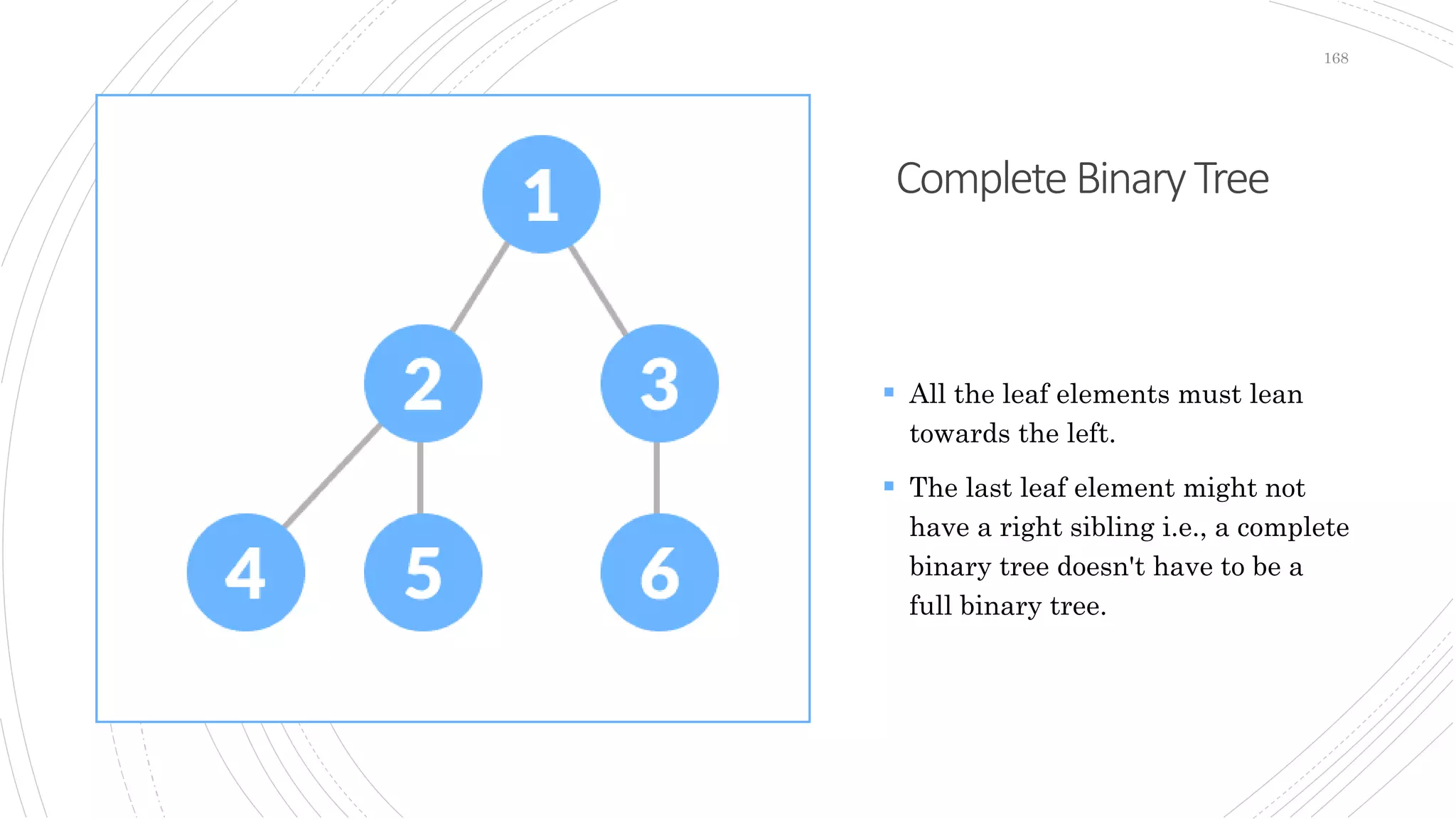
 All the leaf elements must lean
towards the left.
 The last leaf element might not
have a right sibling i.e., a complete
binary tree doesn't have to be a
full binary tree.
Properties
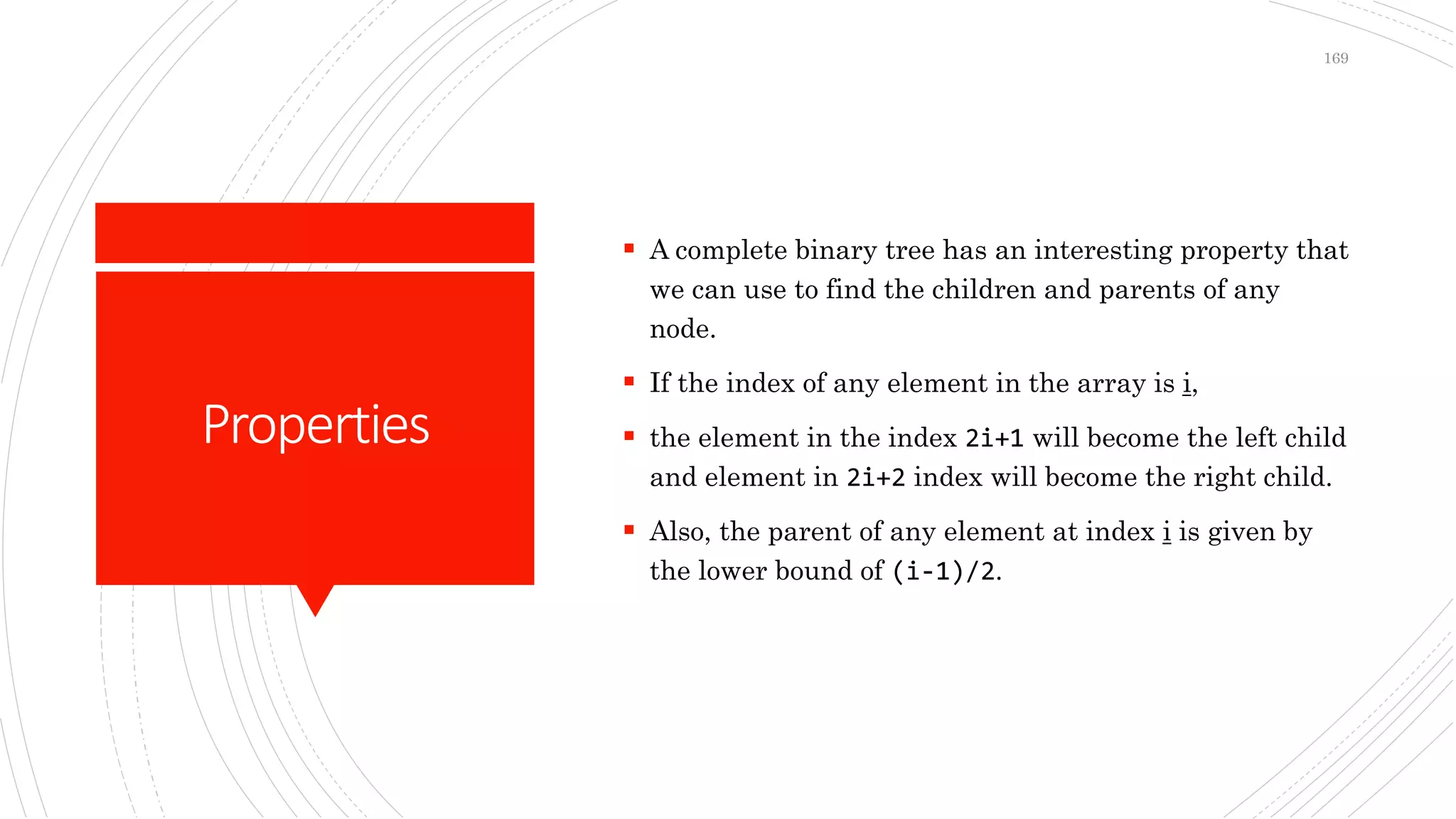
 A complete binary tree has an interesting property that
we can use to find the children and parents of any
node.
 If the index of any element in the array is i,
 the element in the index 2i+1 will become the left child
and element in 2i+2 index will become the right child.
 Also, the parent of any element at index i is given by
the lower bound of (i-1)/2.
169
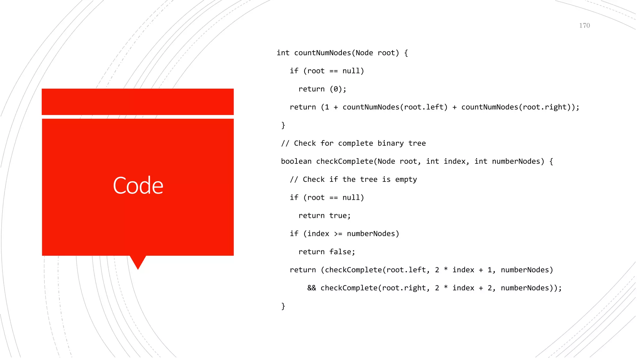
Code
int countNumNodes(Node root) {
if (root == null)
return (0);
return (1 + countNumNodes(root.left) + countNumNodes(root.right));
}
// Check for complete binary tree
boolean checkComplete(Node root, int index, int numberNodes) {
// Check if the tree is empty
if (root == null)
return true;
if (index >= numberNodes)
return false;
return (checkComplete(root.left, 2 * index + 1, numberNodes)
&& checkComplete(root.right, 2 * index + 2, numberNodes));
}
170
BalancedBinaryTree
171
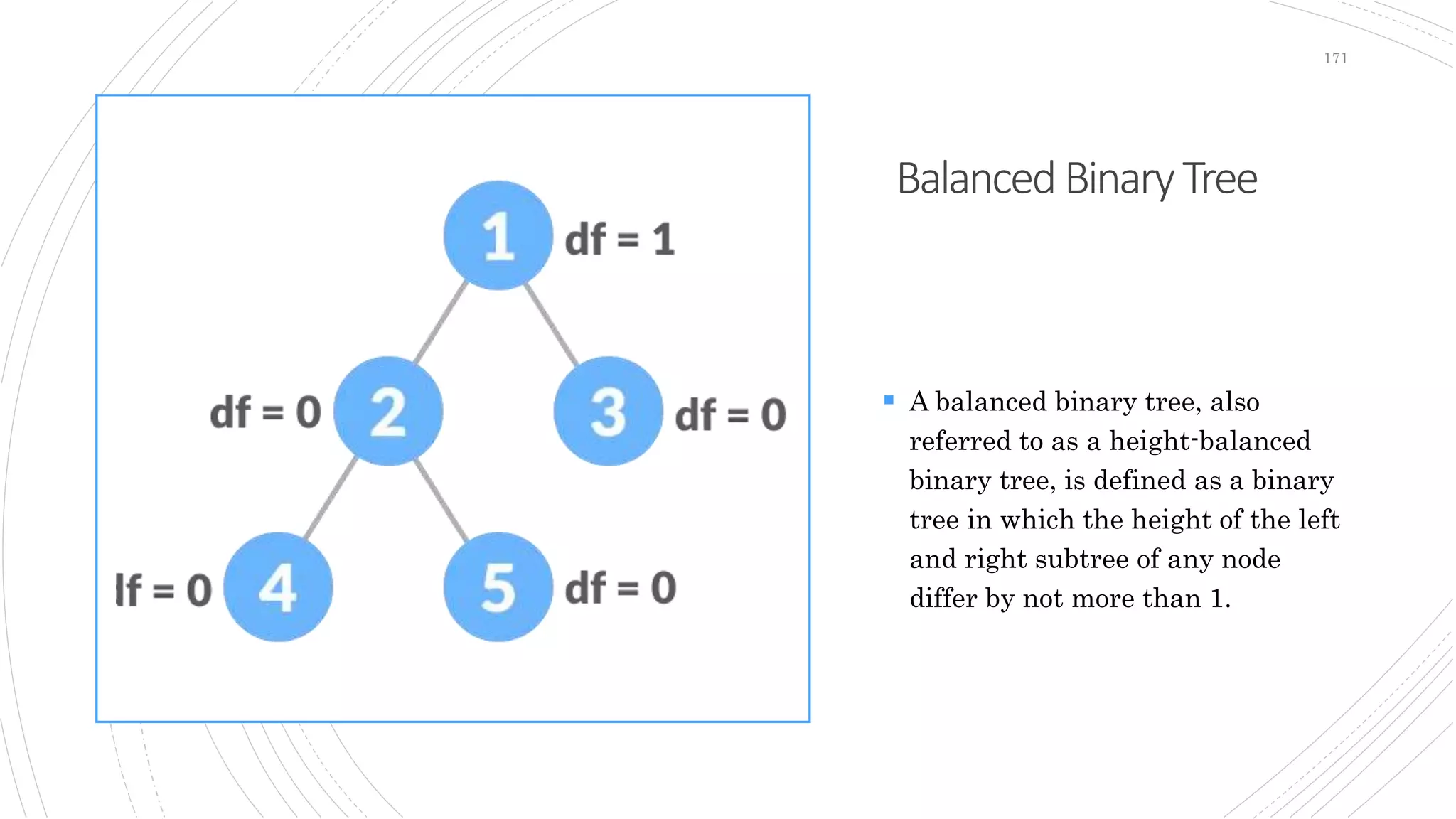
 A balanced binary tree, also
referred to as a height-balanced
binary tree, is defined as a binary
tree in which the height of the left
and right subtree of any node
differ by not more than 1.
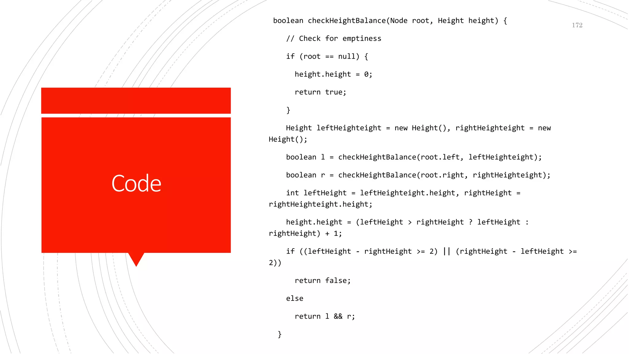
Code
boolean checkHeightBalance(Node root, Height height) {
// Check for emptiness
if (root == null) {
height.height = 0;
return true;
}
Height leftHeighteight = new Height(), rightHeighteight = new
Height();
boolean l = checkHeightBalance(root.left, leftHeighteight);
boolean r = checkHeightBalance(root.right, rightHeighteight);
int leftHeight = leftHeighteight.height, rightHeight =
rightHeighteight.height;
height.height = (leftHeight > rightHeight ? leftHeight :
rightHeight) + 1;
if ((leftHeight - rightHeight >= 2) || (rightHeight - leftHeight >=
2))
return false;
else
return l && r;
}
172
BinarySearchTree
173
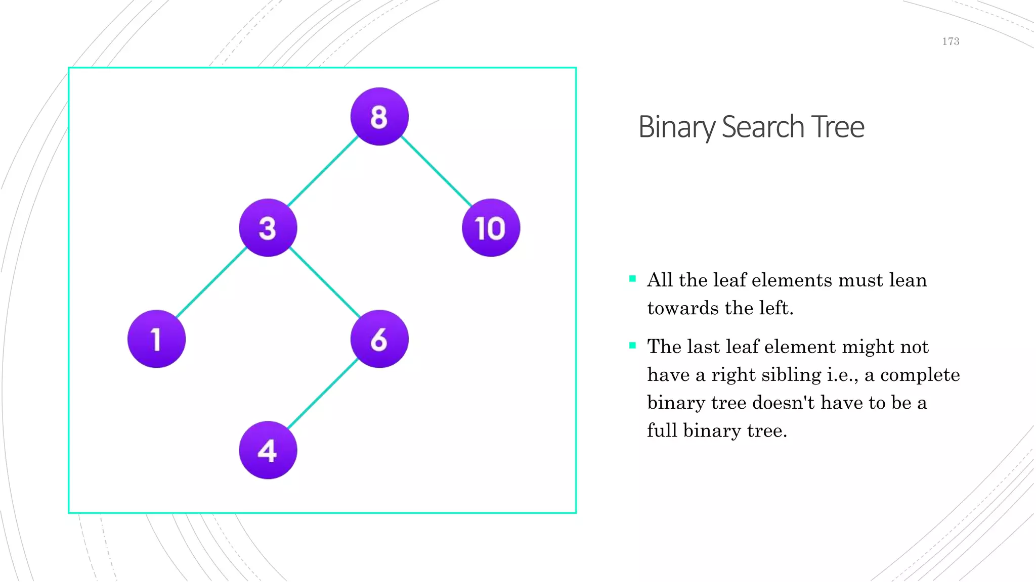
 All the leaf elements must lean
towards the left.
 The last leaf element might not
have a right sibling i.e., a complete
binary tree doesn't have to be a
full binary tree.
Properties
 All nodes of left subtree are less than the root node
 All nodes of right subtree are more than the root node
 Both subtrees of each node are also BSTs i.e. they have
the above two properties
174
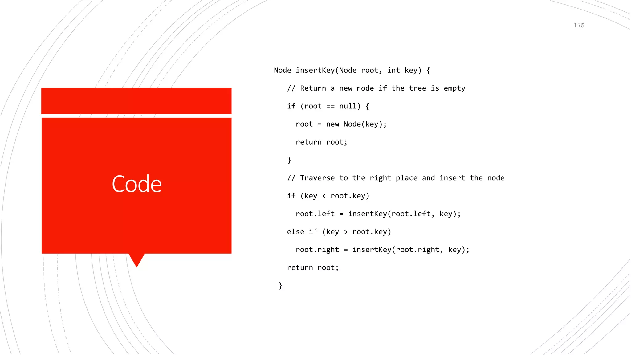
Code
Node insertKey(Node root, int key) {
// Return a new node if the tree is empty
if (root == null) {
root = new Node(key);
return root;
}
// Traverse to the right place and insert the node
if (key < root.key)
root.left = insertKey(root.left, key);
else if (key > root.key)
root.right = insertKey(root.right, key);
return root;
}
175
Adelson-Velsky and
LandisTree
176
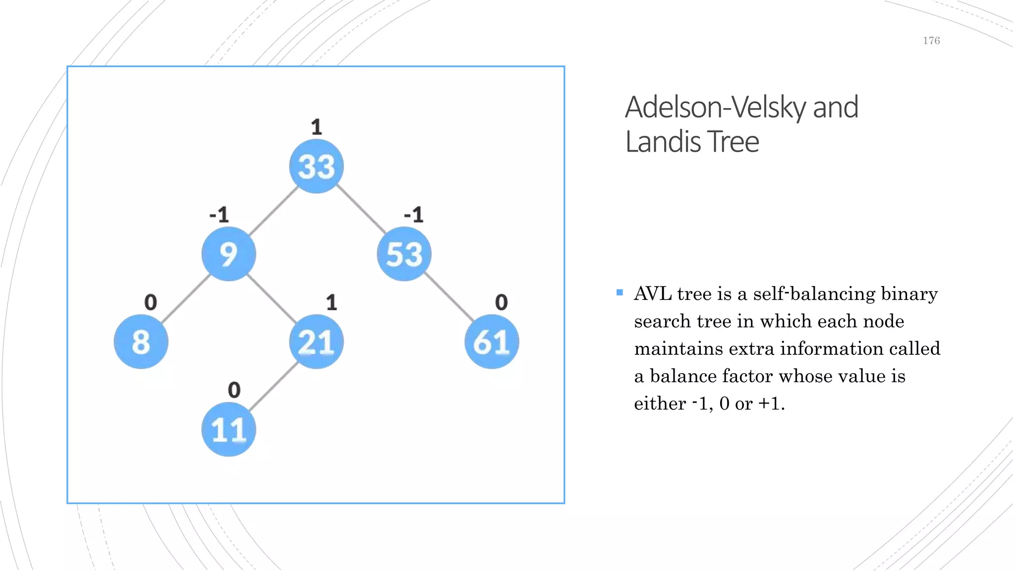
 AVL tree is a self-balancing binary
search tree in which each node
maintains extra information called
a balance factor whose value is
either -1, 0 or +1.
Rotation
Operation
 Left Rotate
 Right Rotate
 Left-Right Rotate
 Right-Left Rotate
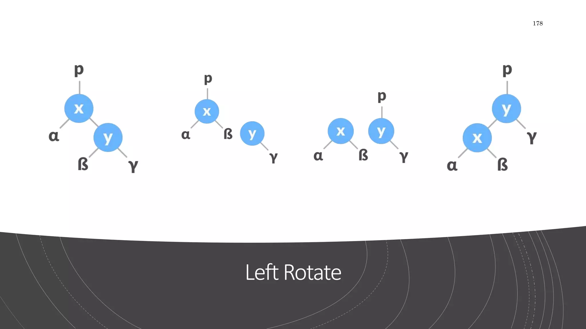
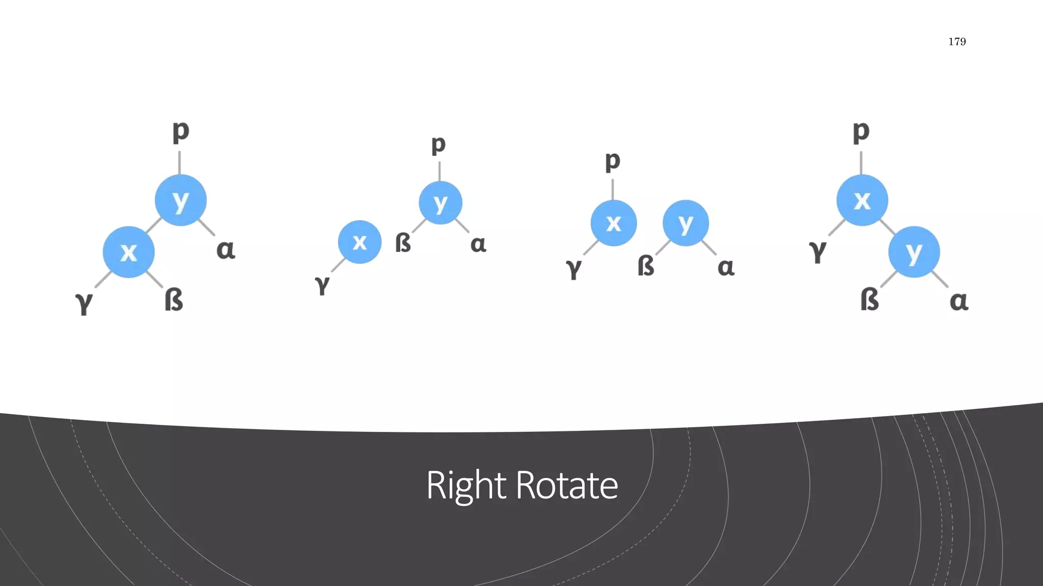
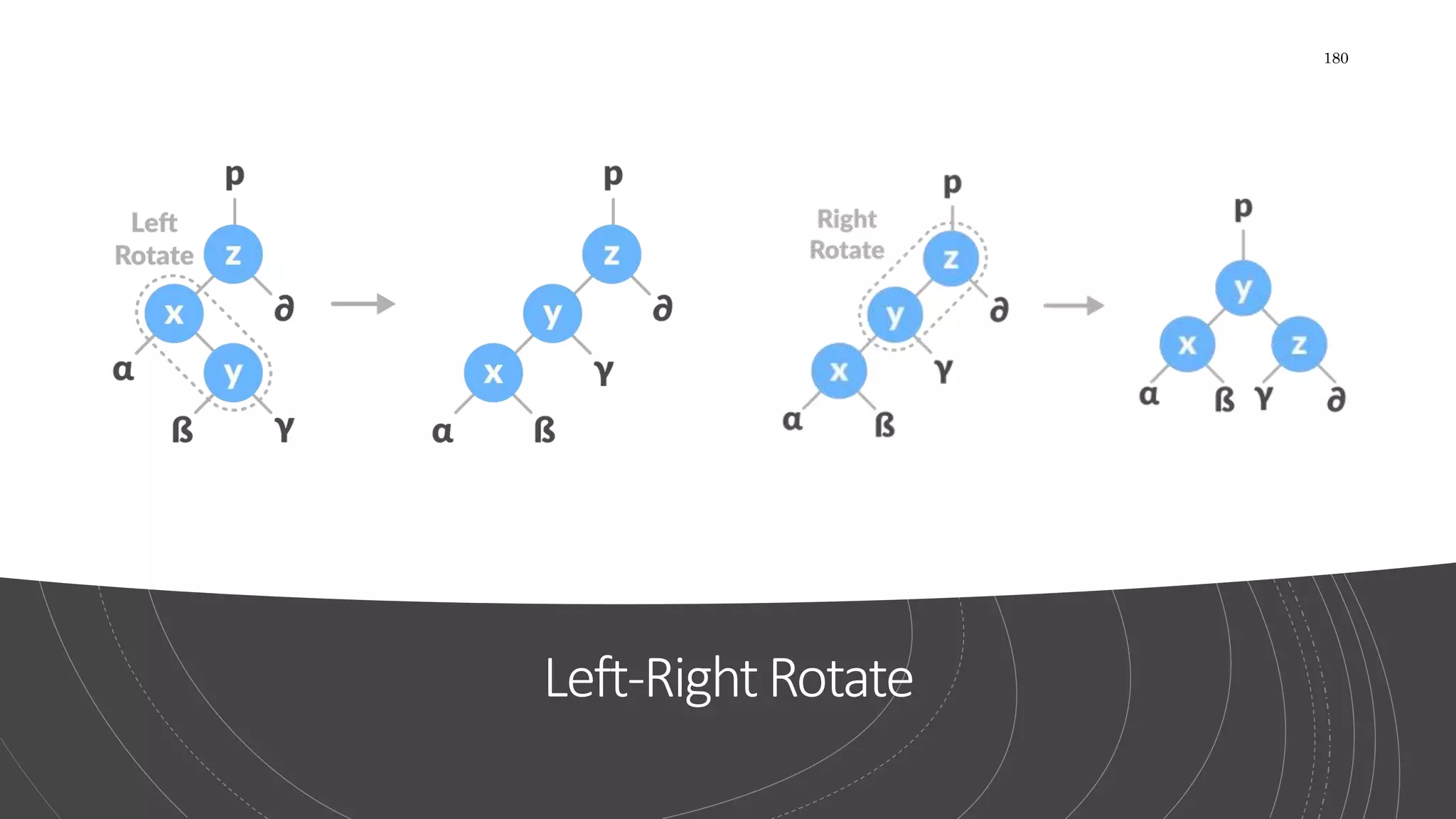
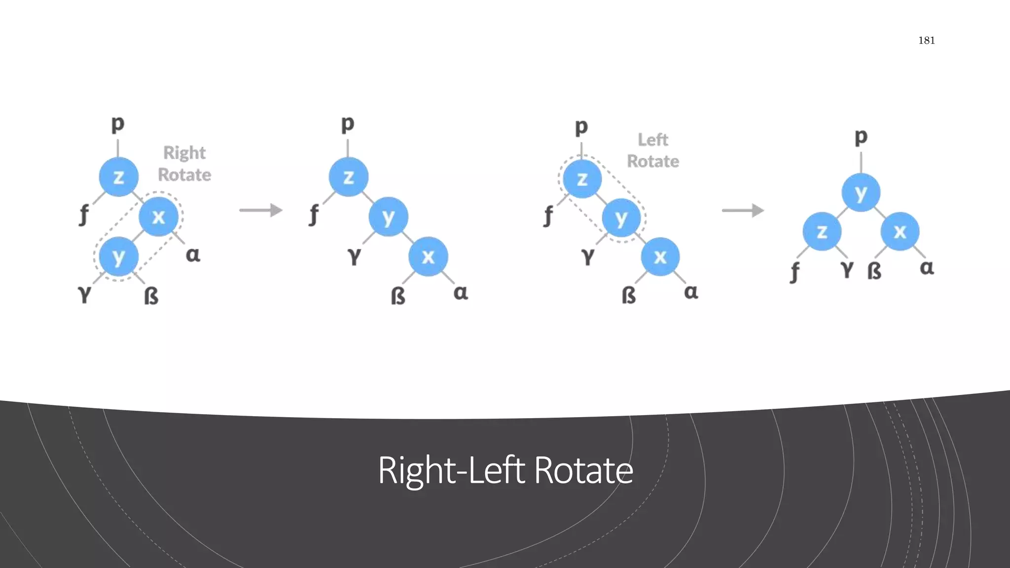
177
LeftRotate
178
RightRotate
179
Left-RightRotate
180
Right-LeftRotate
181
WhentoRotate
182
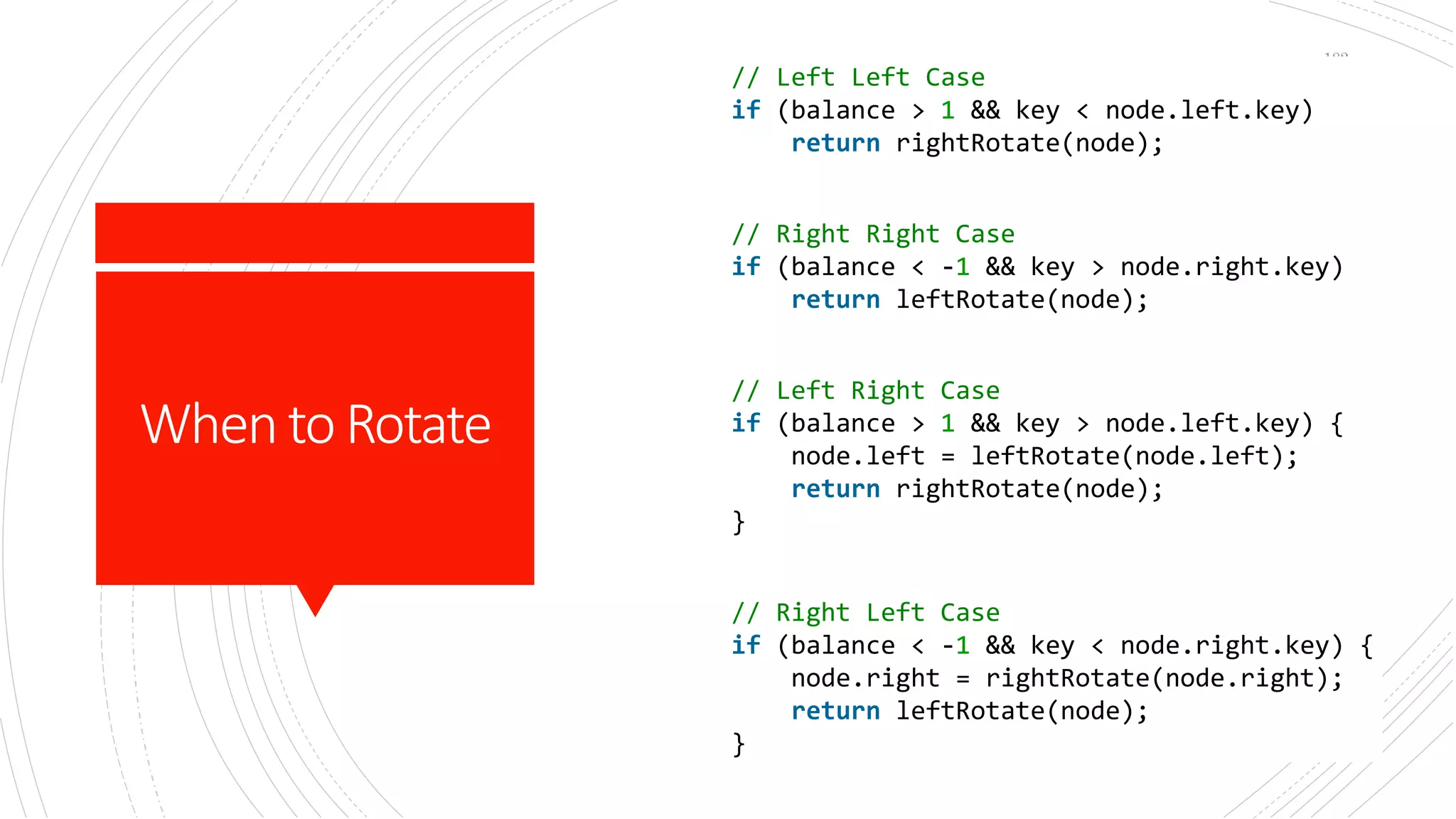
// Left Left Case
if (balance > 1 && key < node.left.key)
return rightRotate(node);
// Right Right Case
if (balance < -1 && key > node.right.key)
return leftRotate(node);
// Left Right Case
if (balance > 1 && key > node.left.key) {
node.left = leftRotate(node.left);
return rightRotate(node);
}
// Right Left Case
if (balance < -1 && key < node.right.key) {
node.right = rightRotate(node.right);
return leftRotate(node);
}
RightRotate
183
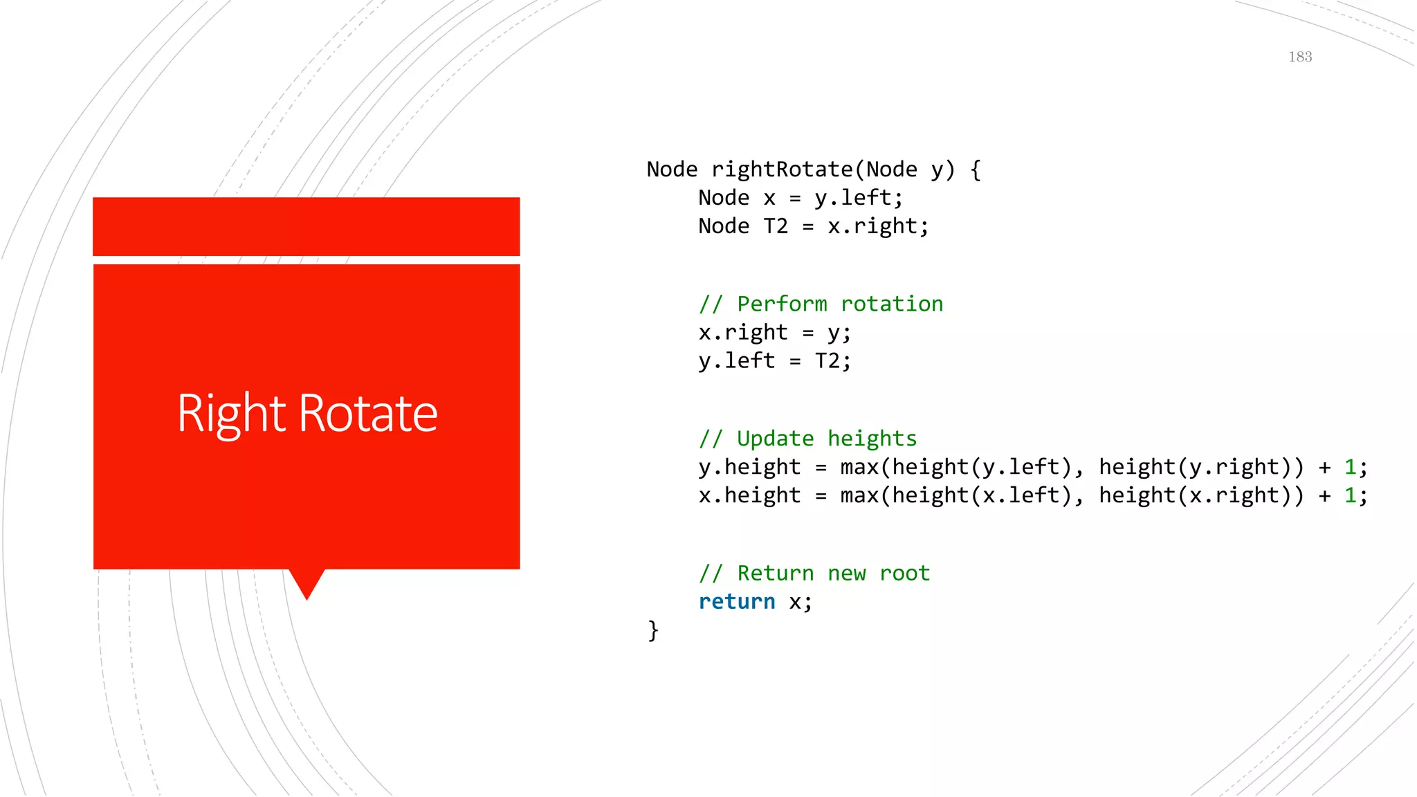
Node rightRotate(Node y) {
Node x = y.left;
Node T2 = x.right;
// Perform rotation
x.right = y;
y.left = T2;
// Update heights
y.height = max(height(y.left), height(y.right)) + 1;
x.height = max(height(x.left), height(x.right)) + 1;
// Return new root
return x;
}
LeftRotate
184
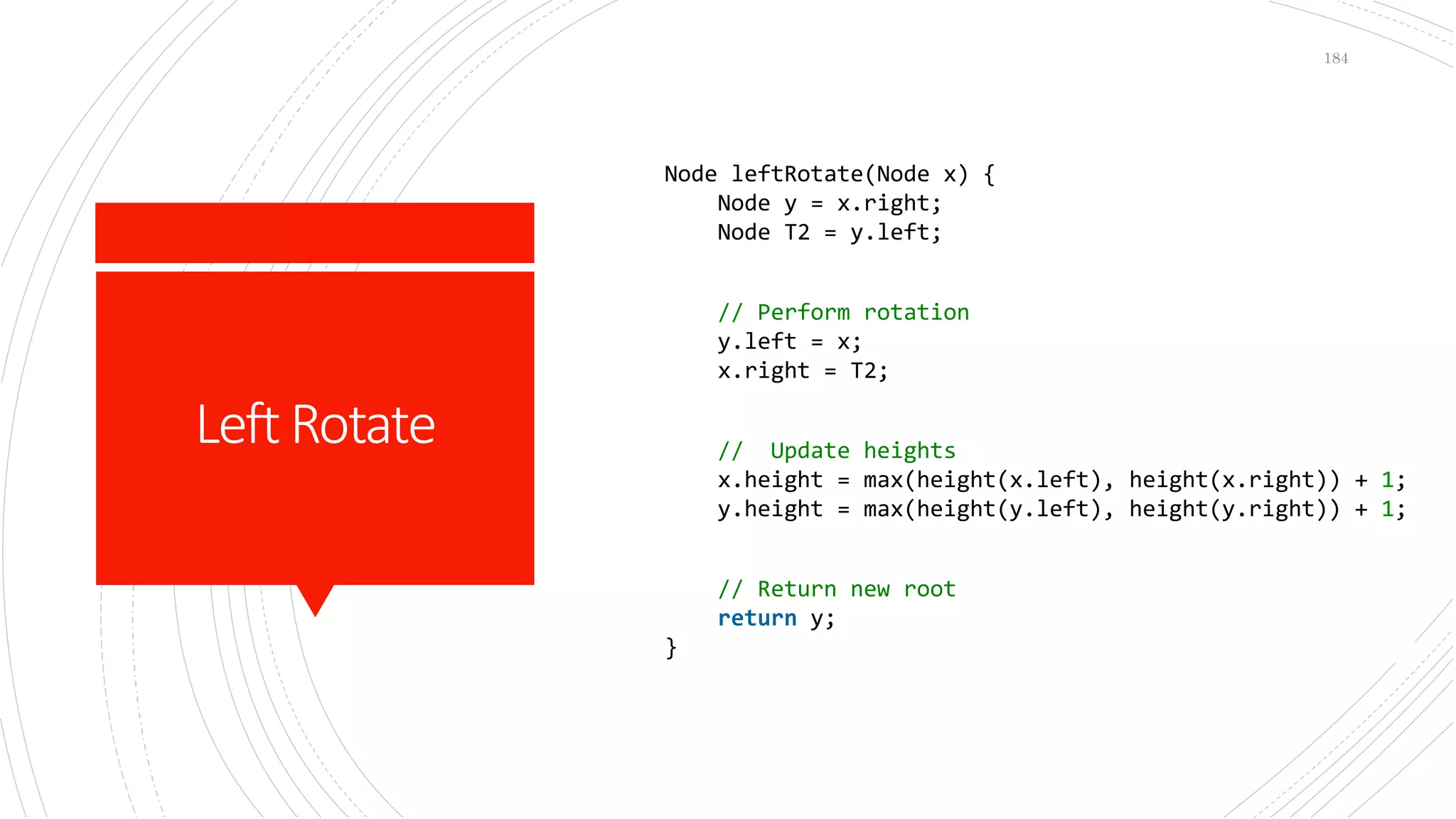
Node leftRotate(Node x) {
Node y = x.right;
Node T2 = y.left;
// Perform rotation
y.left = x;
x.right = T2;
// Update heights
x.height = max(height(x.left), height(x.right)) + 1;
y.height = max(height(y.left), height(y.right)) + 1;
// Return new root
return y;
}
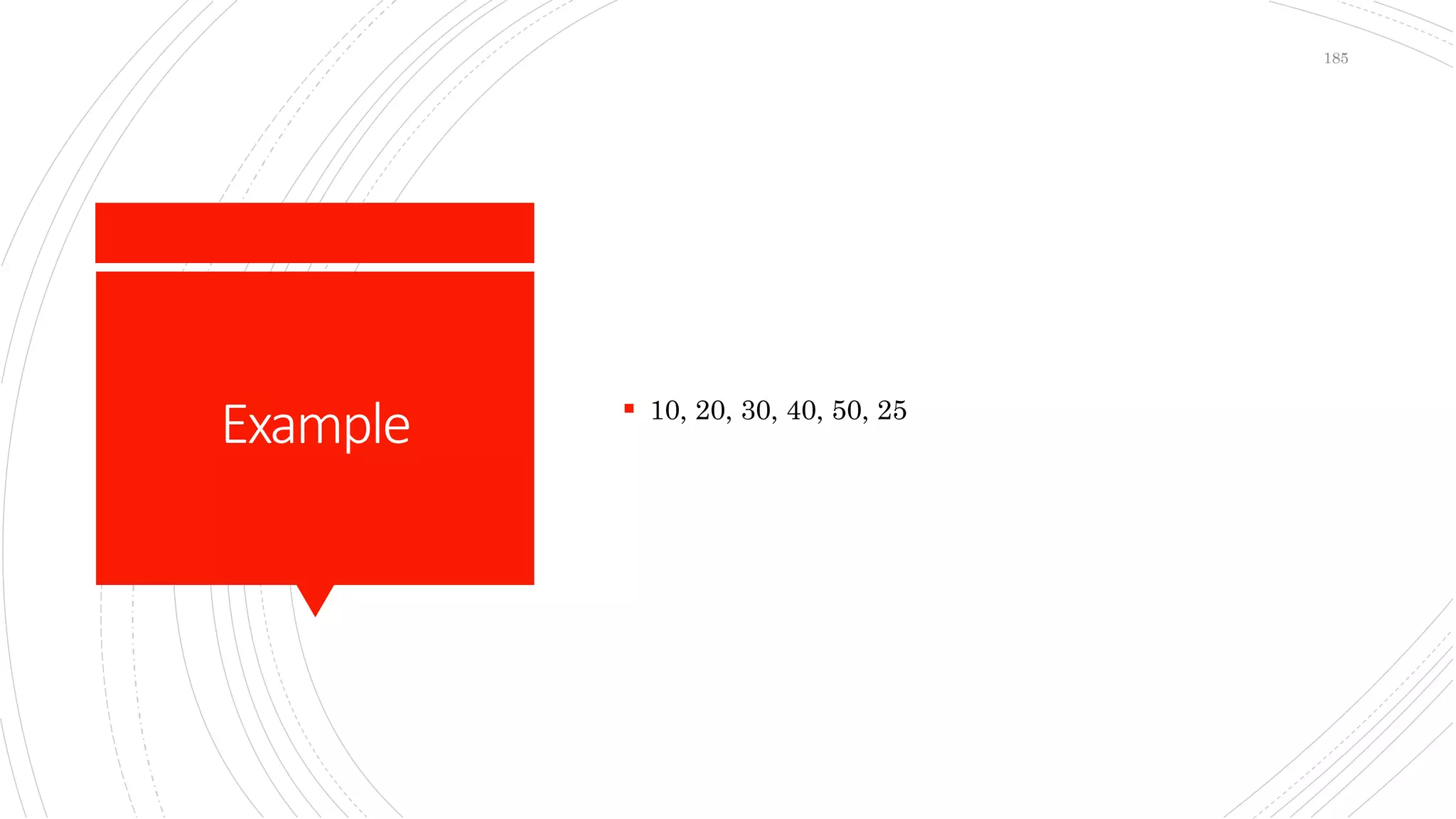
Example  10, 20, 30, 40, 50, 25
185
Graph
186
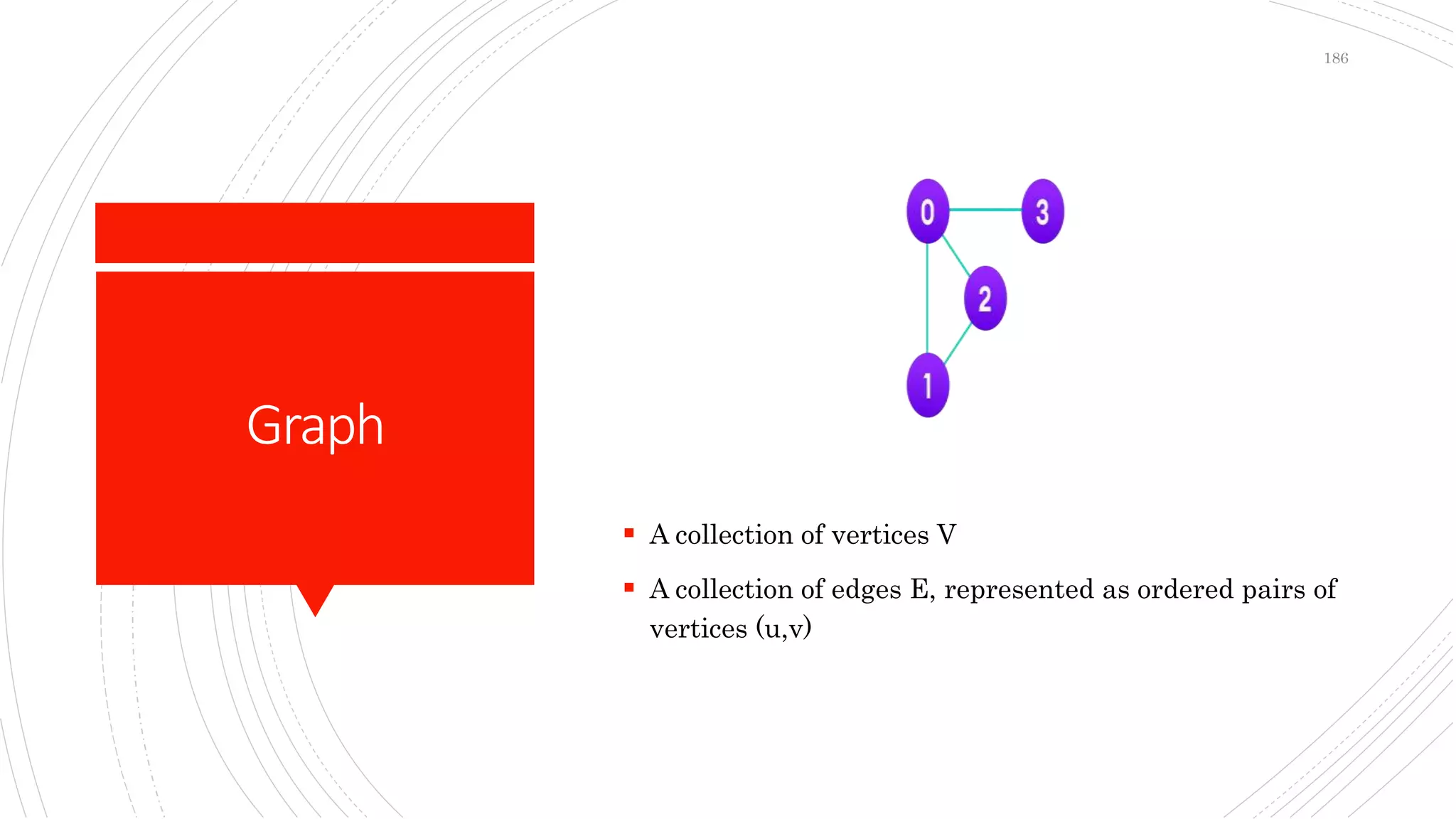
 A collection of vertices V
 A collection of edges E, represented as ordered pairs of
vertices (u,v)
Terminology
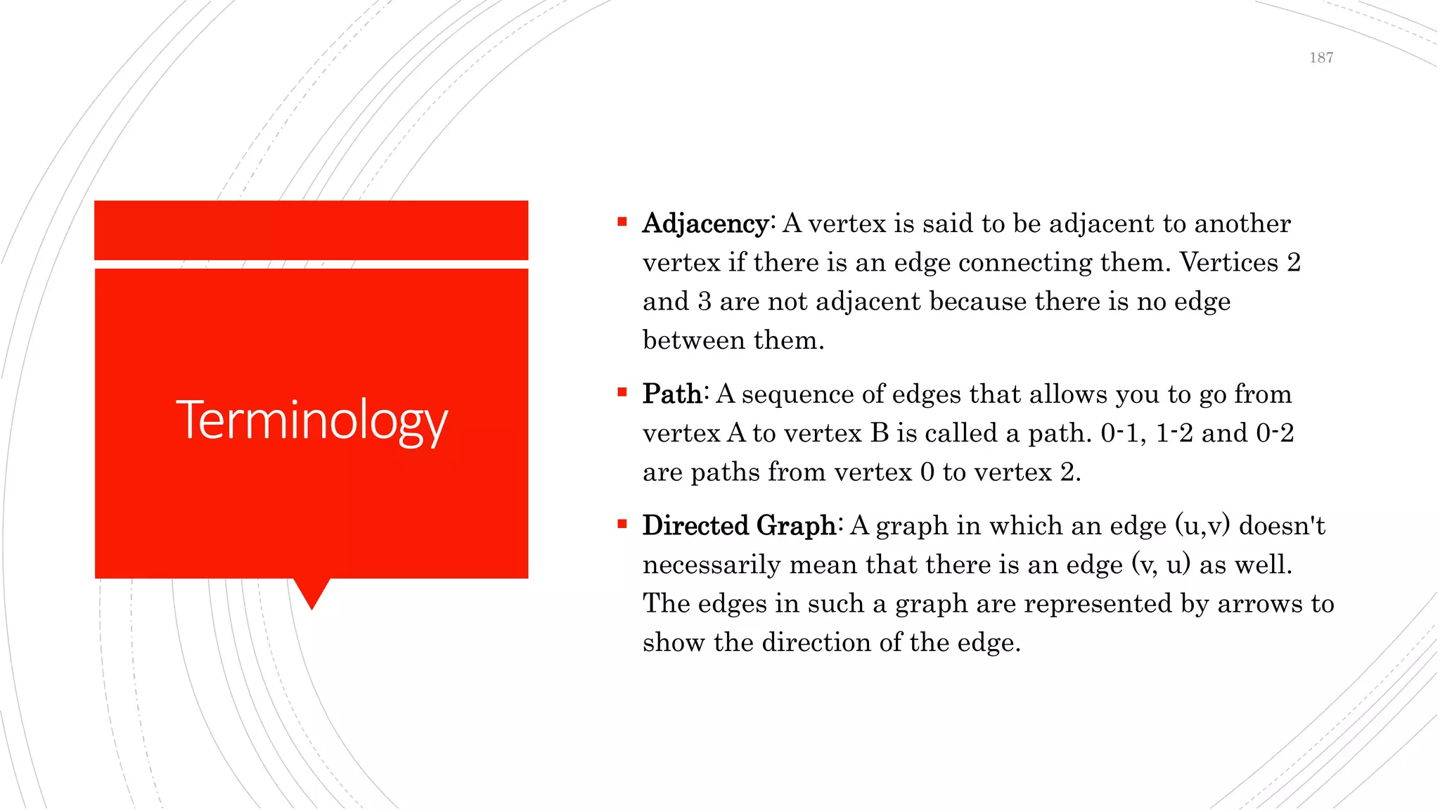
 Adjacency: A vertex is said to be adjacent to another
vertex if there is an edge connecting them. Vertices 2
and 3 are not adjacent because there is no edge
between them.
 Path: A sequence of edges that allows you to go from
vertex A to vertex B is called a path. 0-1, 1-2 and 0-2
are paths from vertex 0 to vertex 2.
 Directed Graph: A graph in which an edge (u,v) doesn't
necessarily mean that there is an edge (v, u) as well.
The edges in such a graph are represented by arrows to
show the direction of the edge.
187
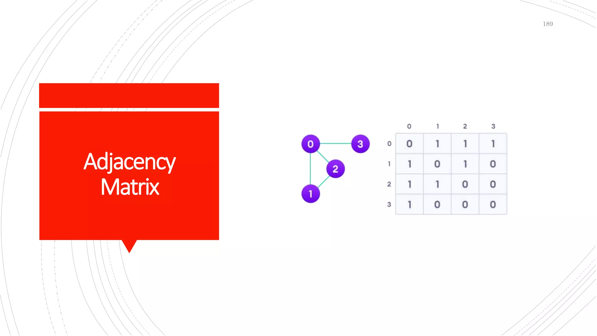
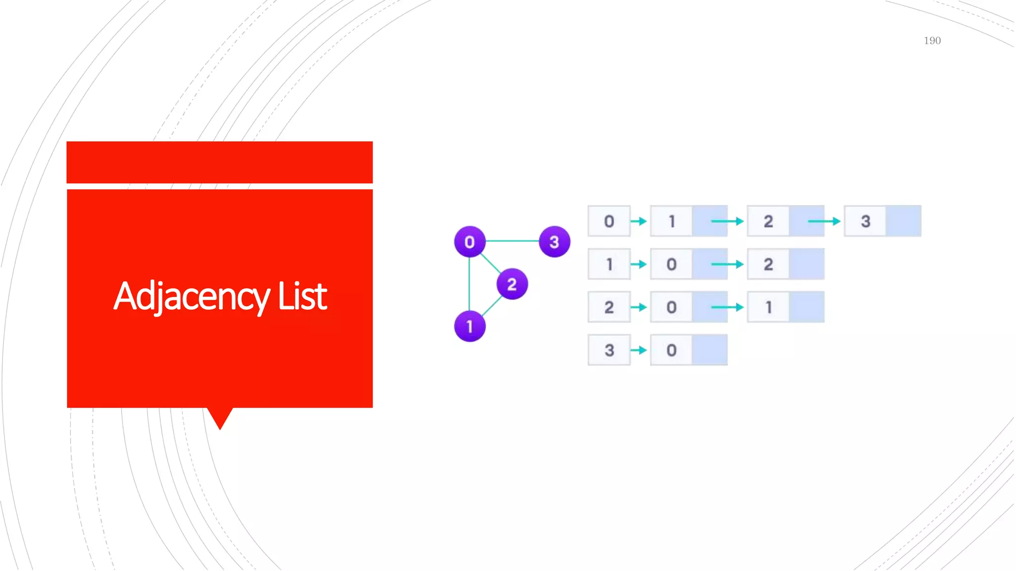
Representation
 Adjacency Matrix: An adjacency matrix is a 2D array of
V x V vertices. Each row and column represent a
vertex.
 Adjacency List: An adjacency list represents a graph as
an array of linked lists.
188
Adjacency
Matrix
189
AdjacencyList
190
SpanningTree
 A spanning tree is a sub-graph of an undirected
connected graph, which includes all the vertices of the
graph with a minimum possible number of edges. If a
vertex is missed, then it is not a spanning tree.
 The edges may or may not have weights assigned to
them.
 The total number of spanning trees with n vertices
that can be created from a complete graph is equal to
n(n-2).
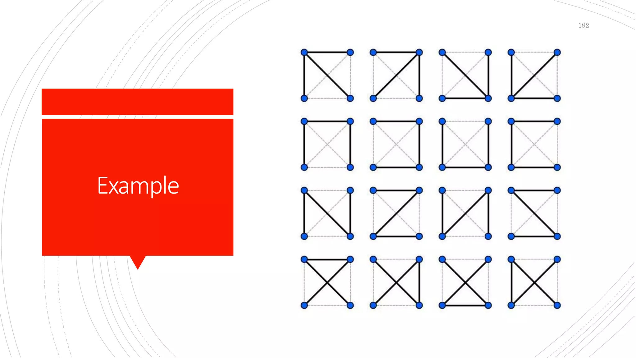
191
Example
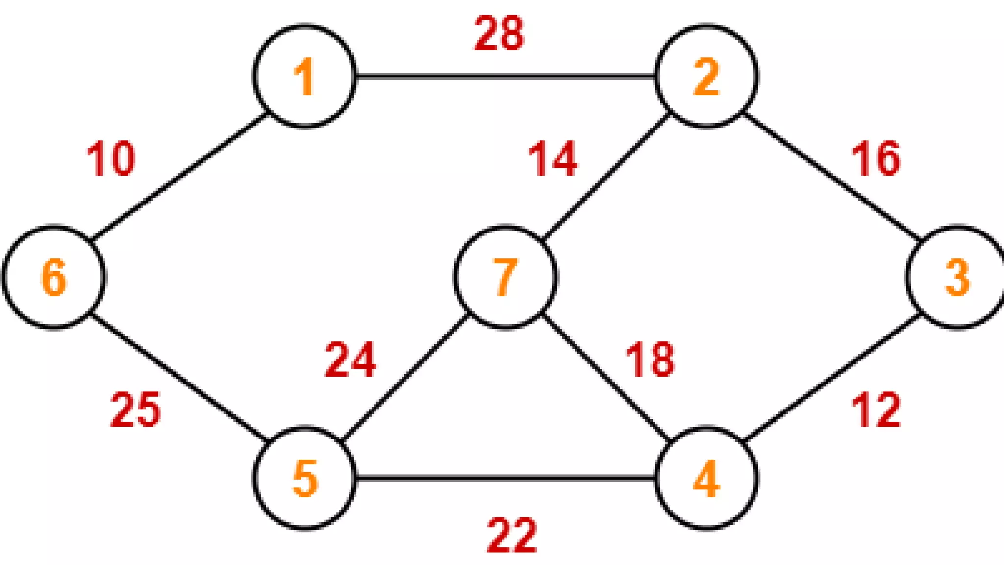
192
Minimum
SpanningTree
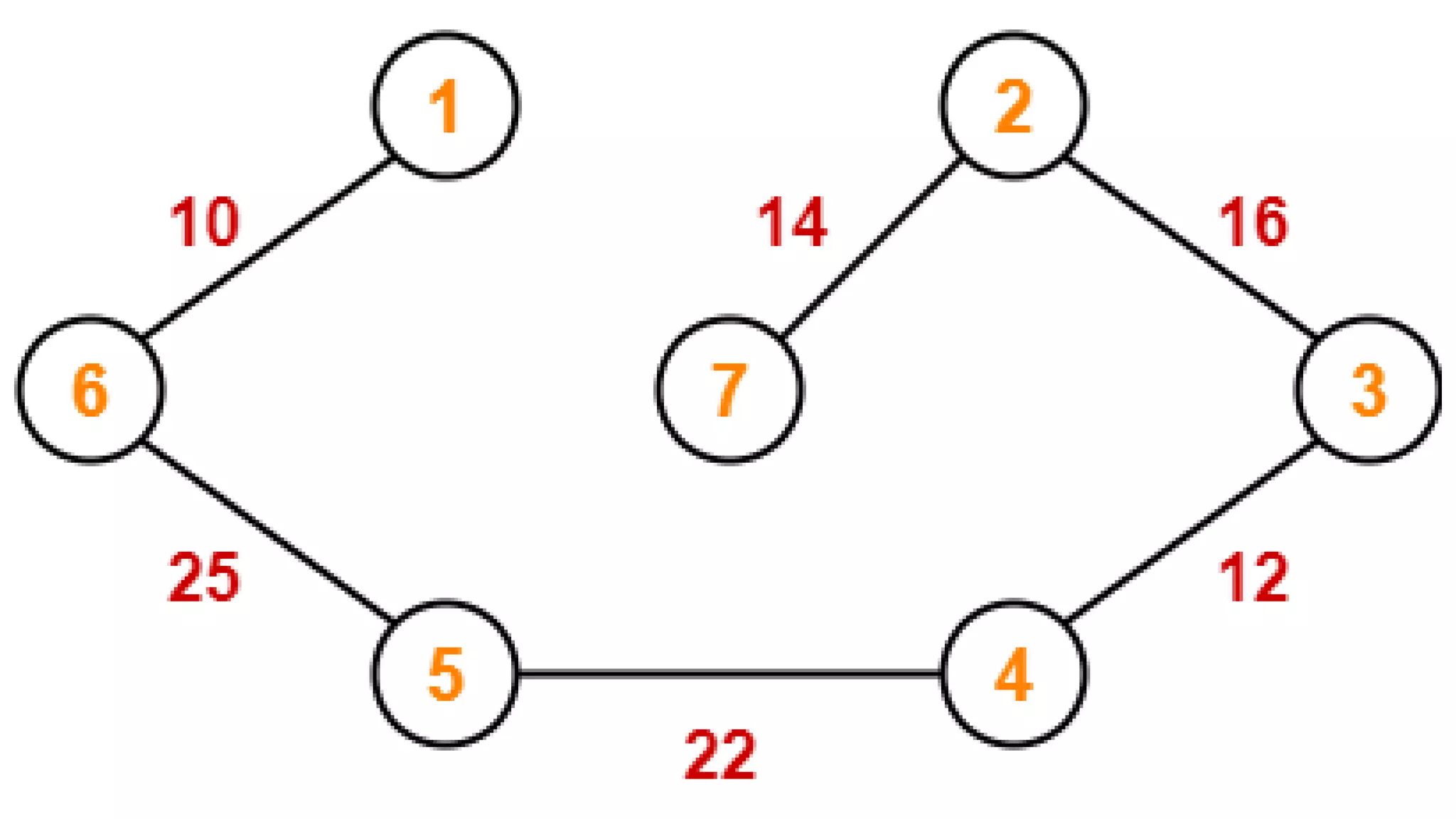
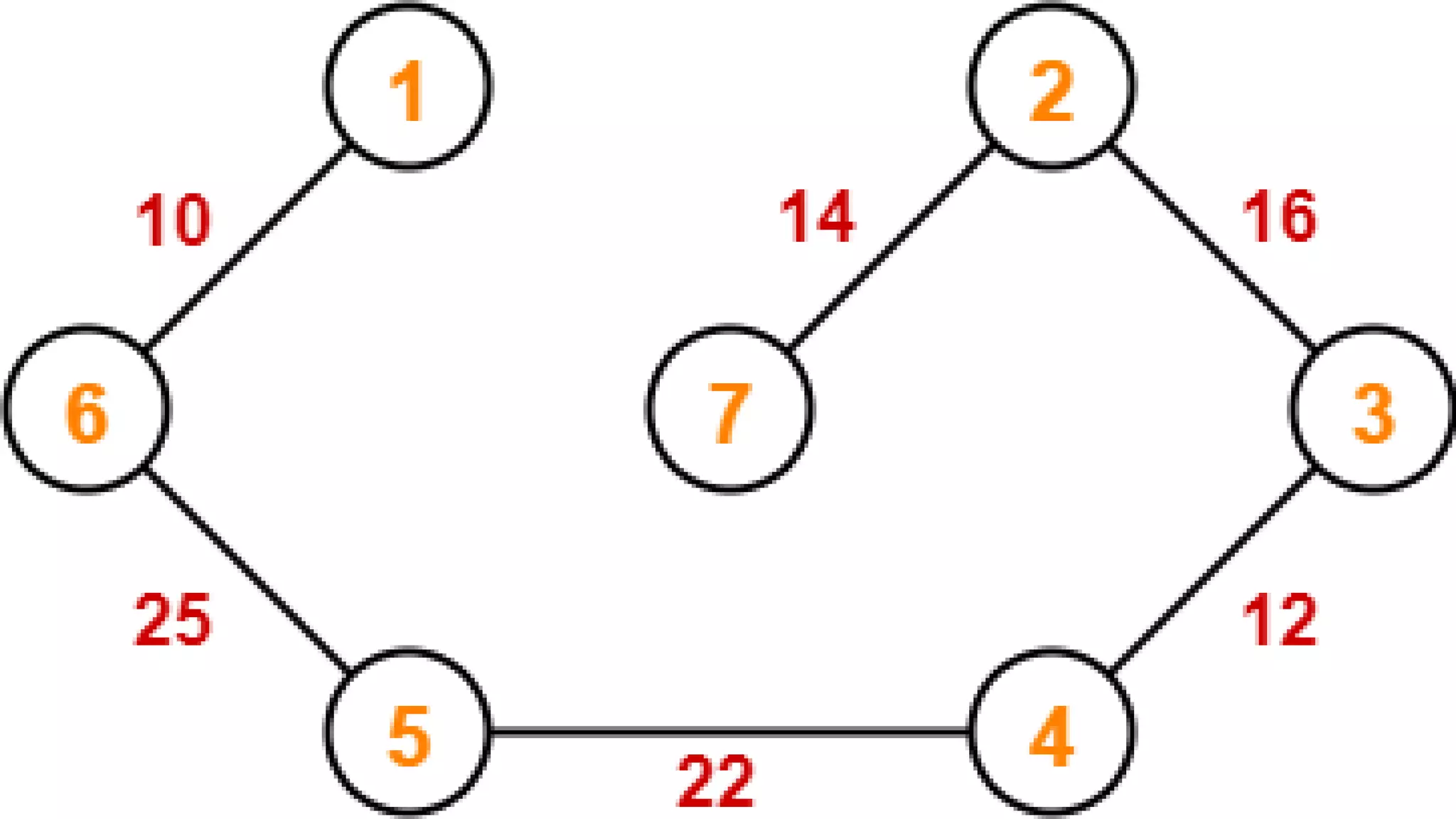
 A minimum spanning tree is a spanning tree in which
the sum of the weight of the edges is as minimum as
possible.
 The minimum spanning tree from a graph is found
using the following algorithms:
 Prim's Algorithm
 Kruskal's Algorithm
193
Prim’s
Algorithm
 Prim's algorithm is a minimum spanning tree
algorithm that takes a graph as input and finds the
subset of the edges of that graph which
 form a tree that includes every vertex
 has the minimum sum of weights among all the trees
that can be formed from the graph
 The steps for implementing Prim's algorithm are as
follows:
 Initialize the minimum spanning tree with a vertex
chosen at random.
 Find all the edges that connect the tree to new vertices,
find the minimum and add it to the tree
 Keep repeating step 2 until we get a minimum spanning
tree
194
"Testing leads to failure,
and failure leads to
understanding."
Burt Rutan
200
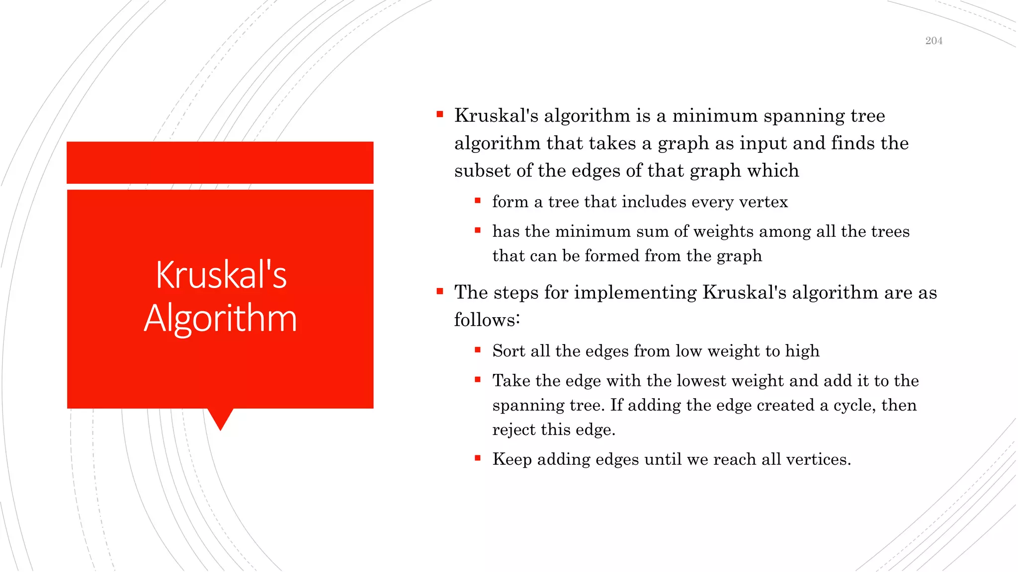
Kruskal's
Algorithm
 Kruskal's algorithm is a minimum spanning tree
algorithm that takes a graph as input and finds the
subset of the edges of that graph which
 form a tree that includes every vertex
 has the minimum sum of weights among all the trees
that can be formed from the graph
 The steps for implementing Kruskal's algorithm are as
follows:
 Sort all the edges from low weight to high
 Take the edge with the lowest weight and add it to the
spanning tree. If adding the edge created a cycle, then
reject this edge.
 Keep adding edges until we reach all vertices.
204
Strongly
Connected
Components
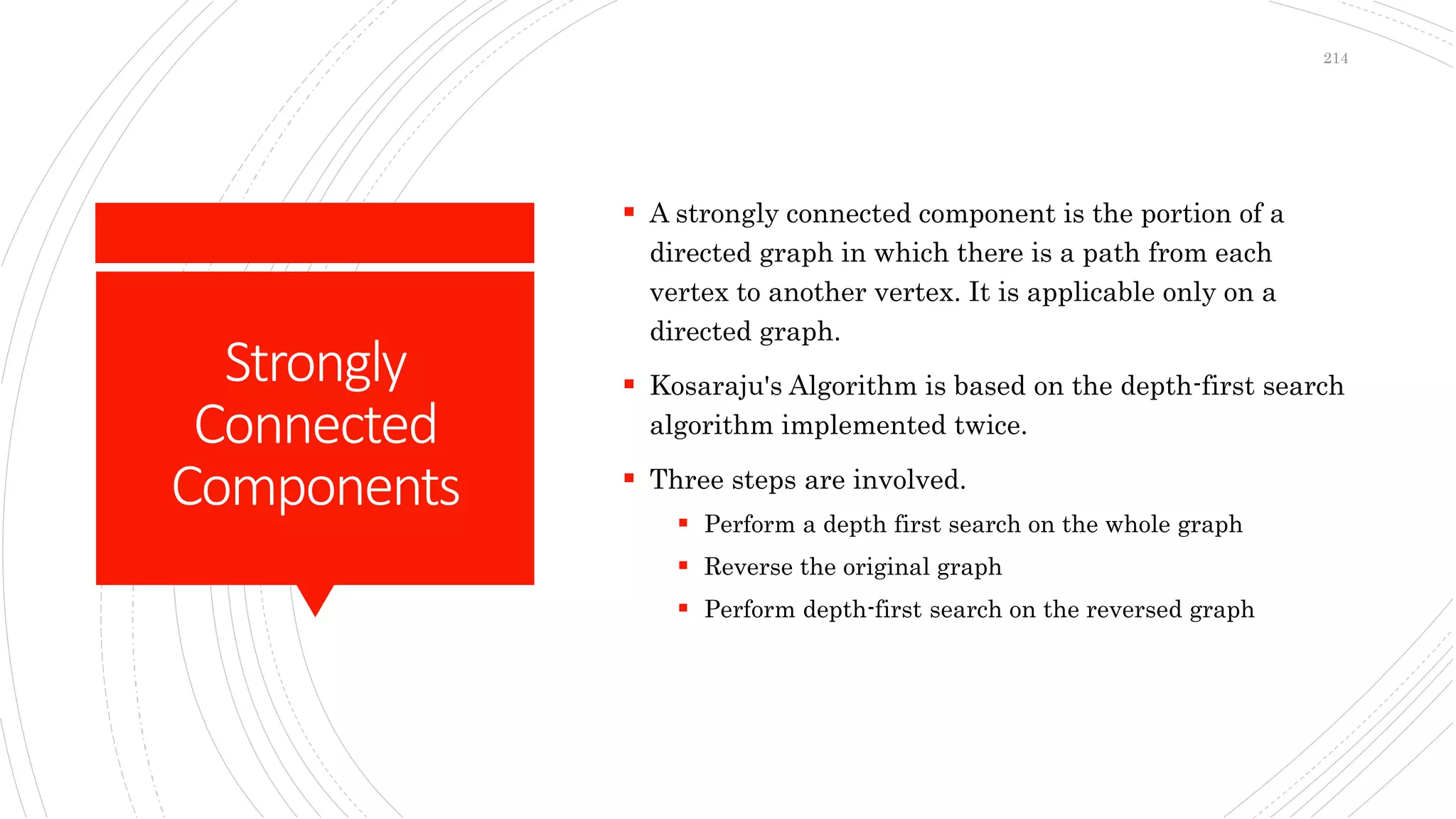
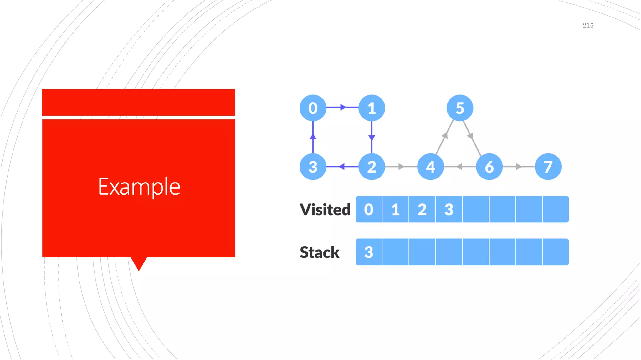
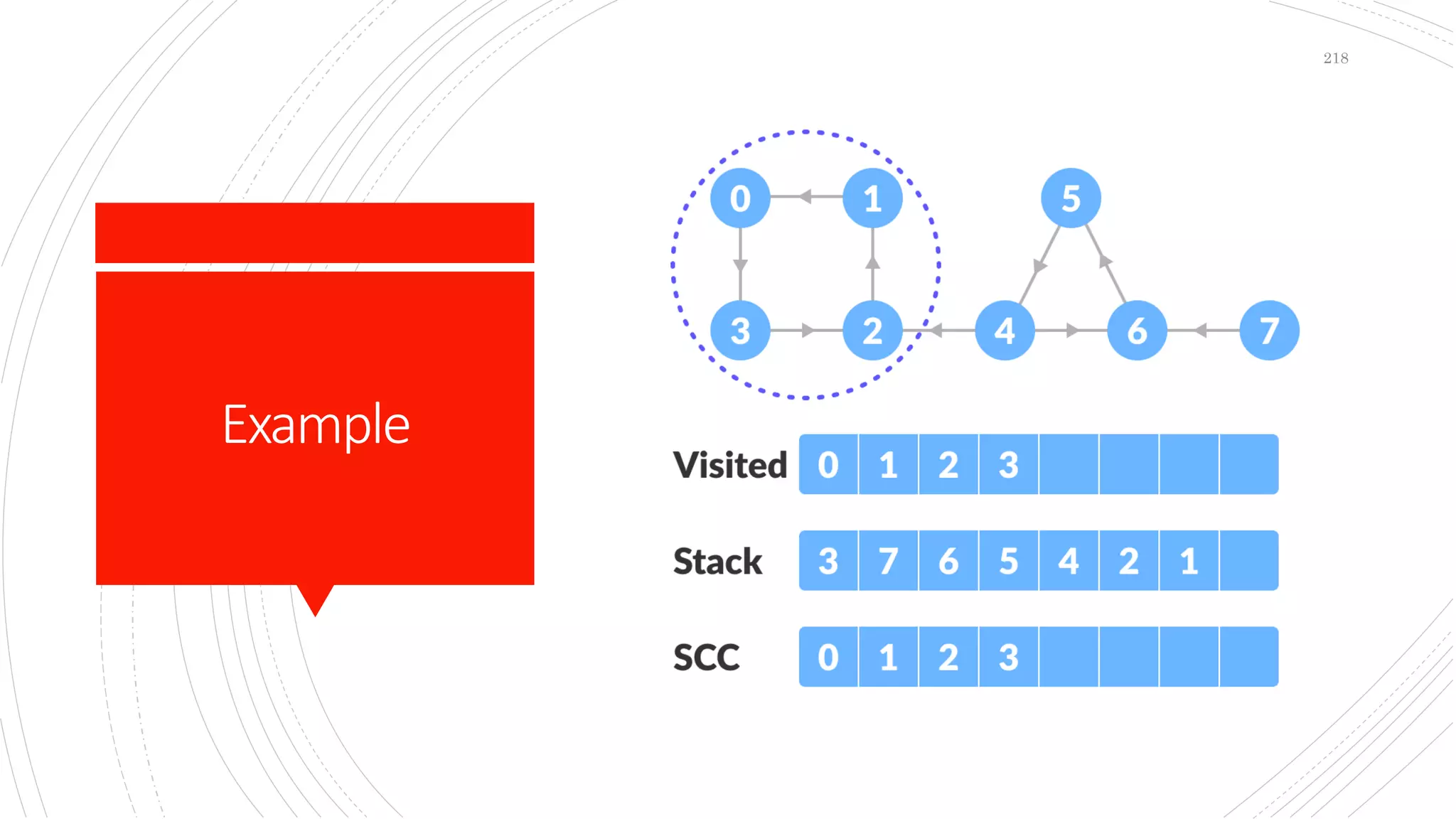
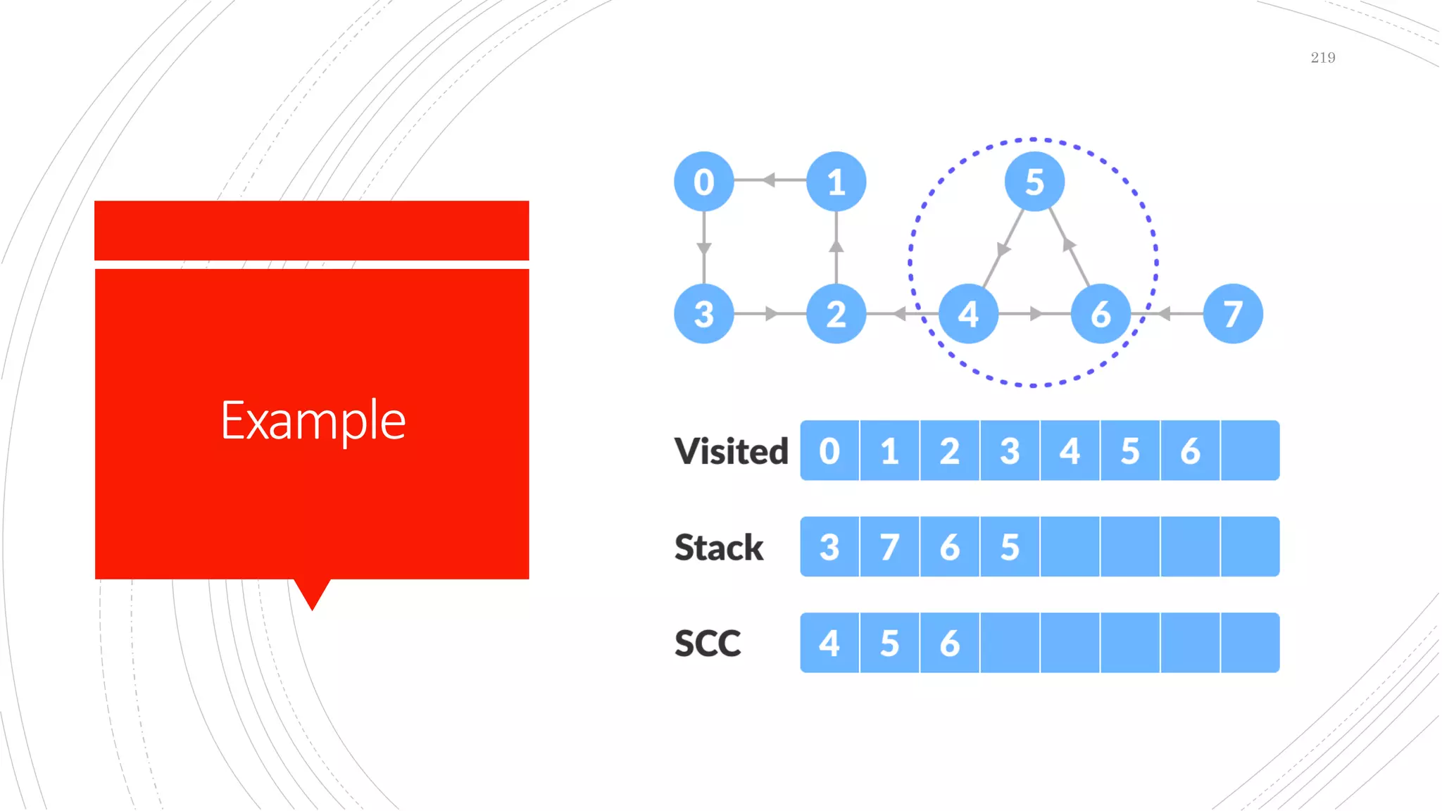
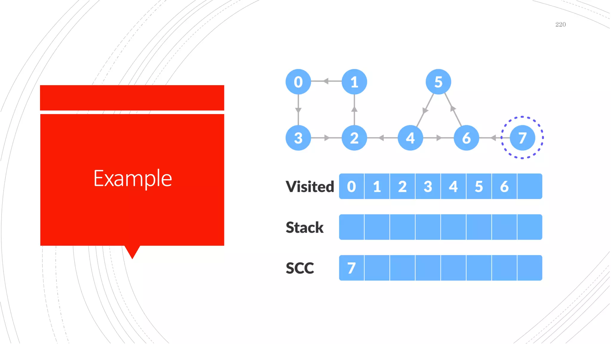
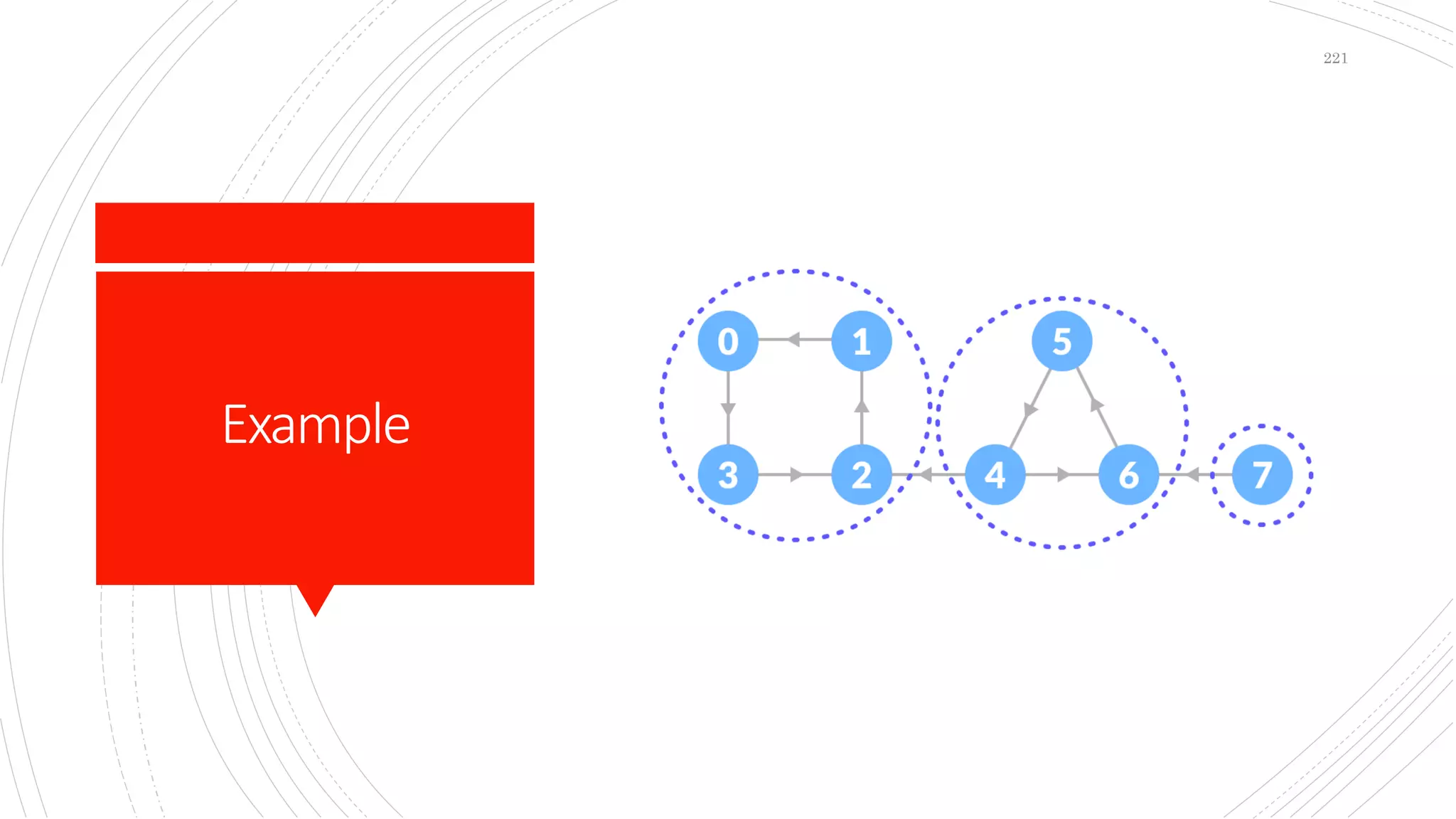
 A strongly connected component is the portion of a
directed graph in which there is a path from each
vertex to another vertex. It is applicable only on a
directed graph.
 Kosaraju's Algorithm is based on the depth-first search
algorithm implemented twice.
 Three steps are involved.
 Perform a depth first search on the whole graph
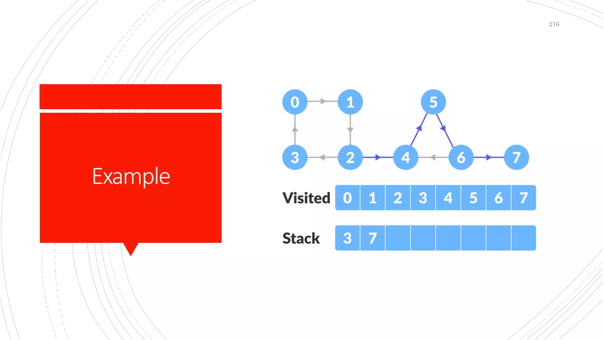
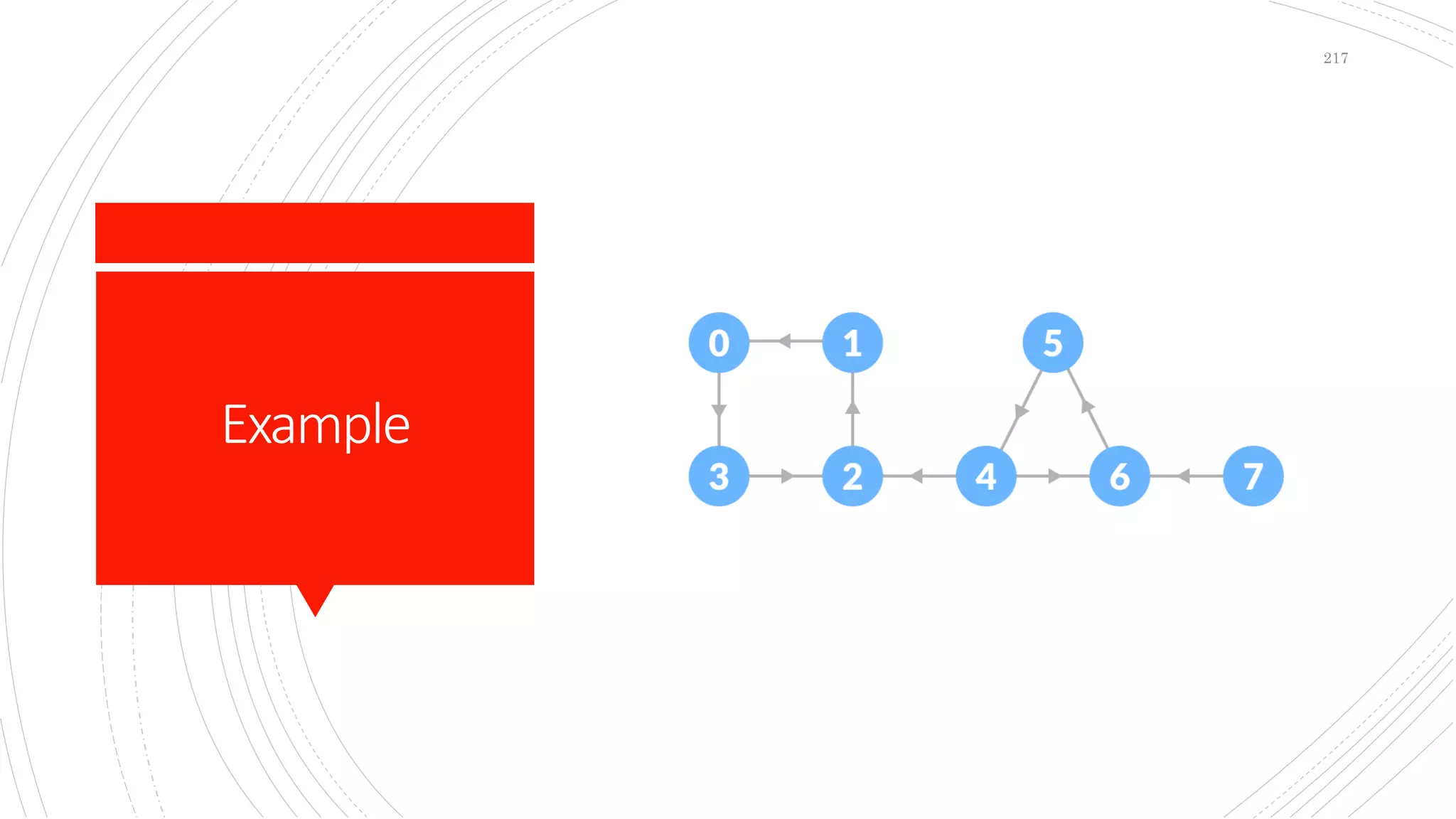
 Reverse the original graph
 Perform depth-first search on the reversed graph
214
Example
215
Example
216
Example
217
Example
218
Example
219
Example
220
Example
221
DepthFirst
Search
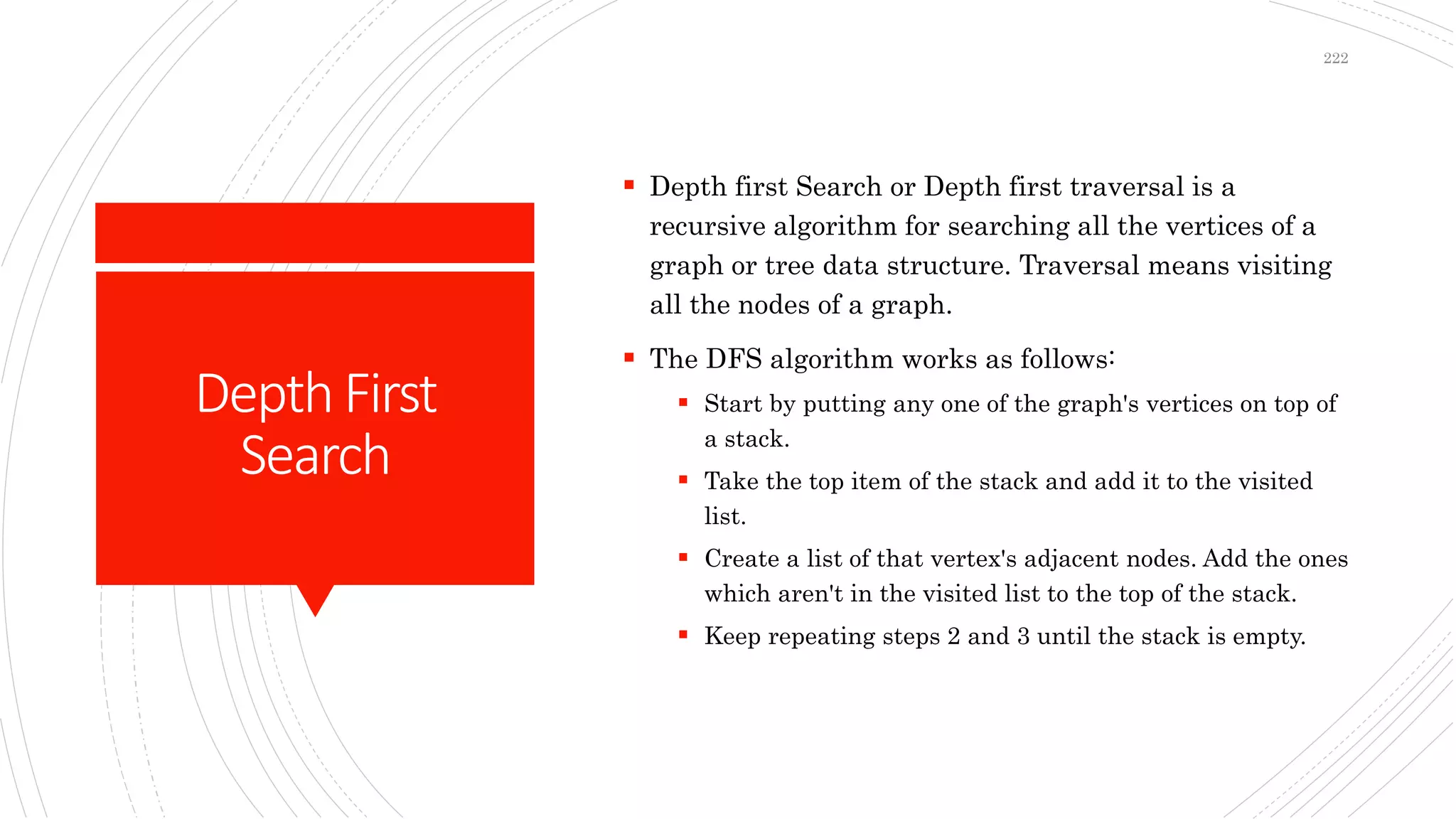
 Depth first Search or Depth first traversal is a
recursive algorithm for searching all the vertices of a
graph or tree data structure. Traversal means visiting
all the nodes of a graph.
 The DFS algorithm works as follows:
 Start by putting any one of the graph's vertices on top of
a stack.
 Take the top item of the stack and add it to the visited
list.
 Create a list of that vertex's adjacent nodes. Add the ones
which aren't in the visited list to the top of the stack.
 Keep repeating steps 2 and 3 until the stack is empty.
222
Breadthfirst
search
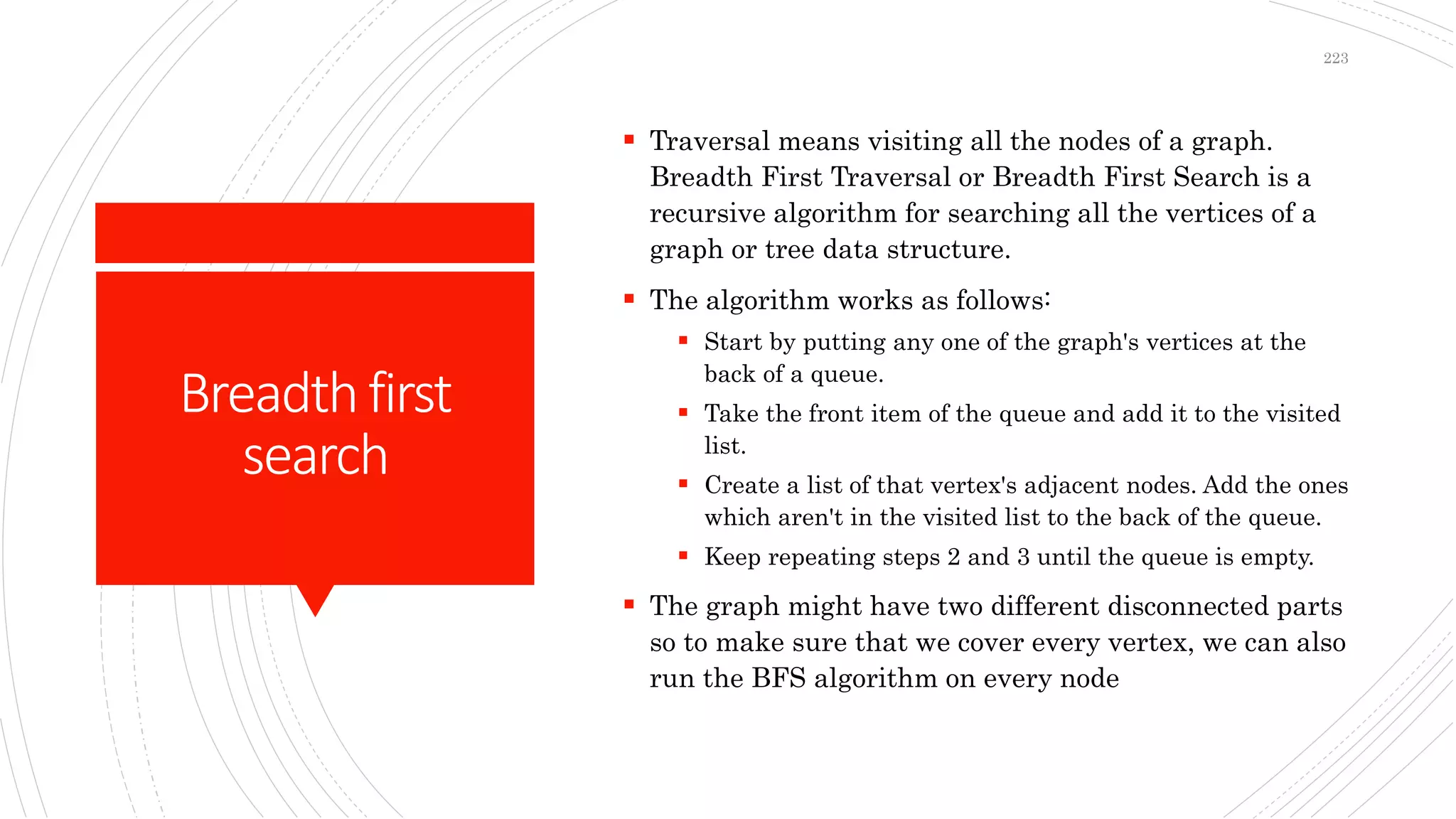
 Traversal means visiting all the nodes of a graph.
Breadth First Traversal or Breadth First Search is a
recursive algorithm for searching all the vertices of a
graph or tree data structure.
 The algorithm works as follows:
 Start by putting any one of the graph's vertices at the
back of a queue.
 Take the front item of the queue and add it to the visited
list.
 Create a list of that vertex's adjacent nodes. Add the ones
which aren't in the visited list to the back of the queue.
 Keep repeating steps 2 and 3 until the queue is empty.
 The graph might have two different disconnected parts
so to make sure that we cover every vertex, we can also
run the BFS algorithm on every node
223
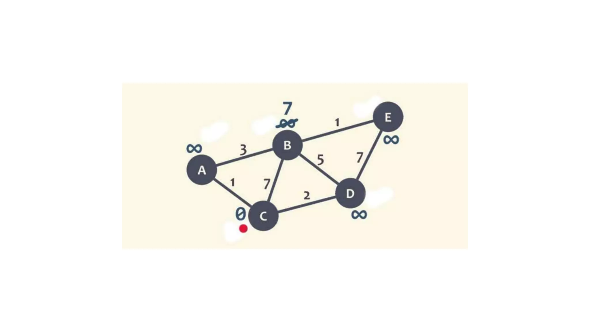
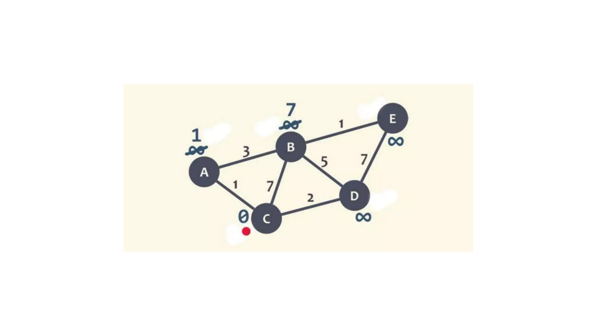
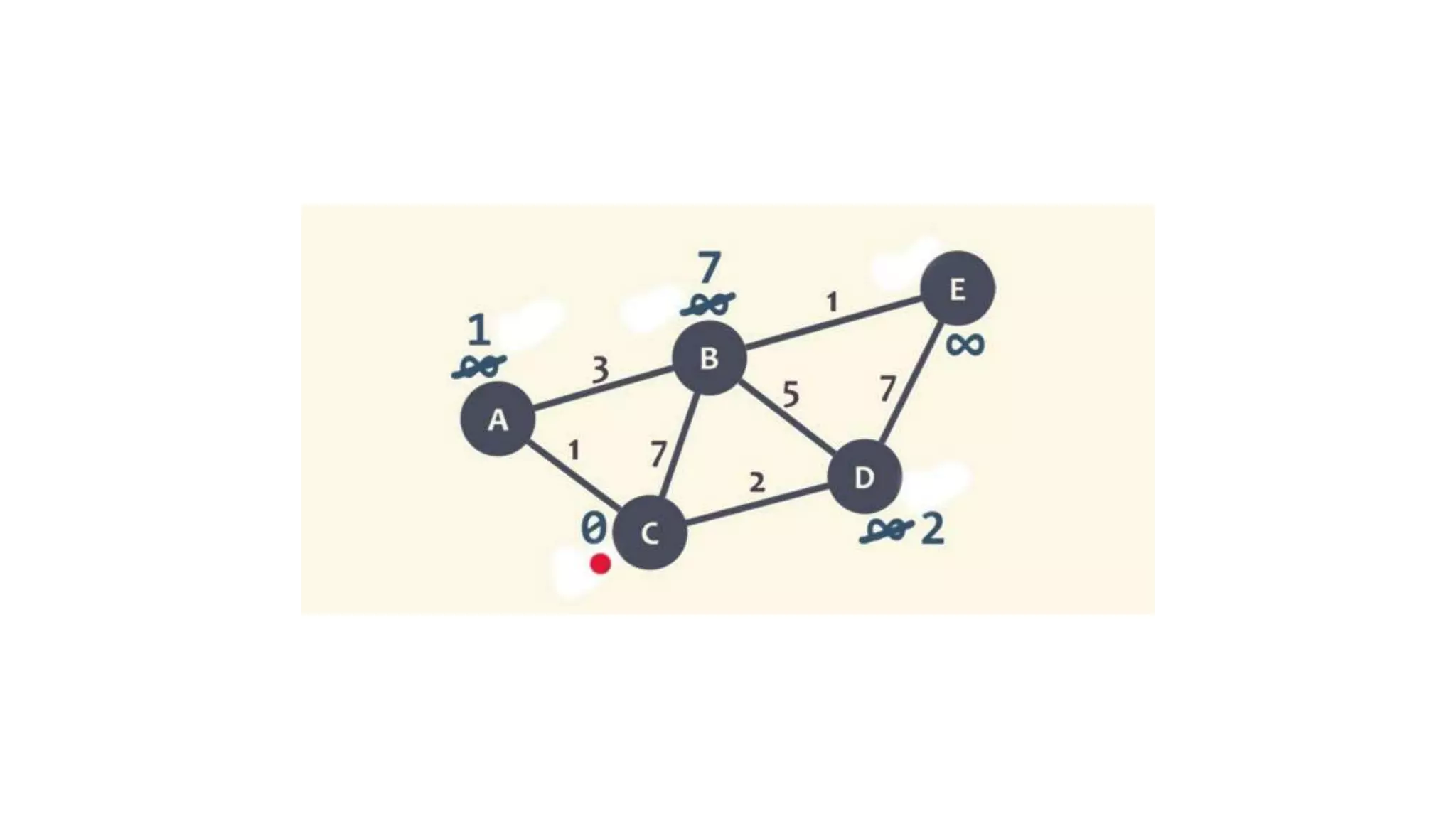
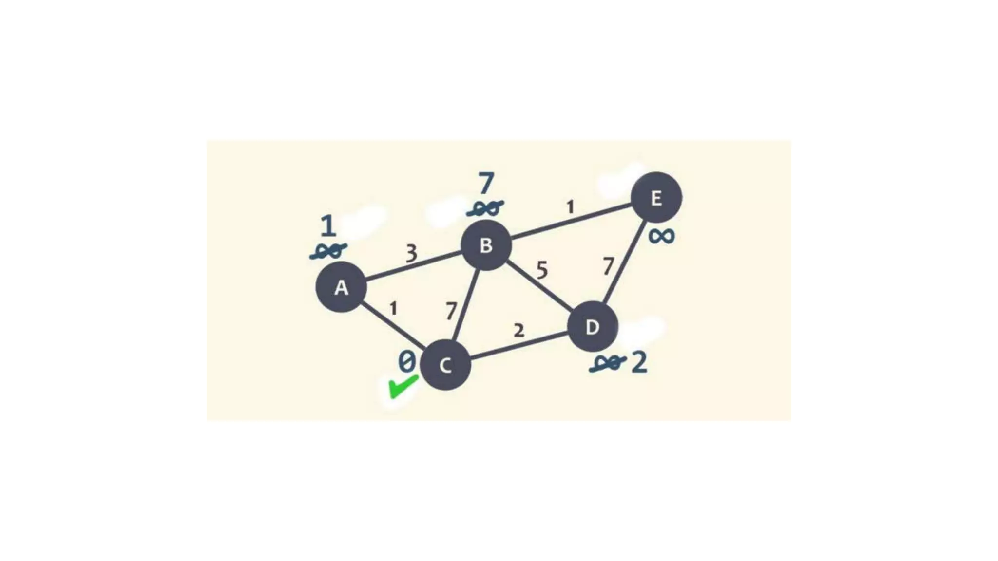
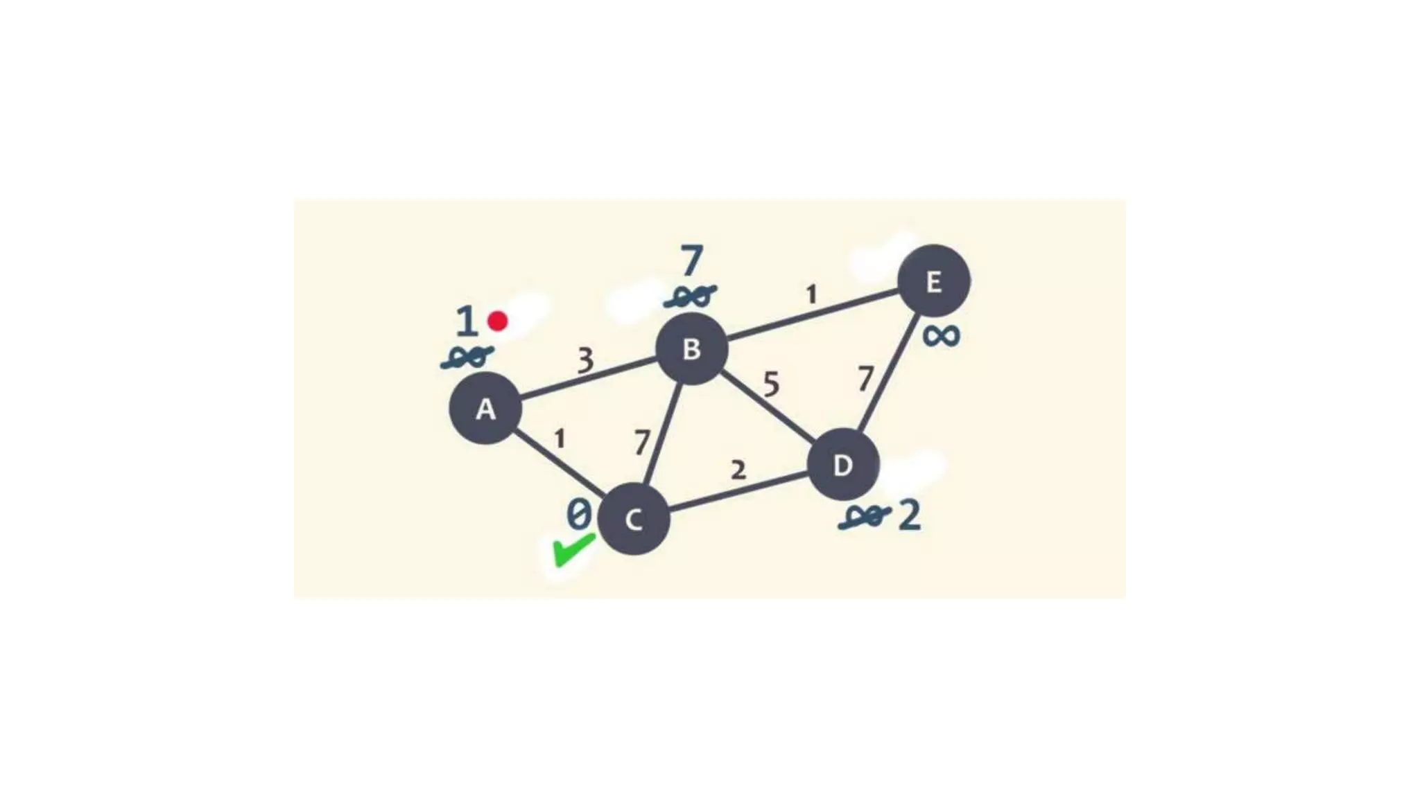
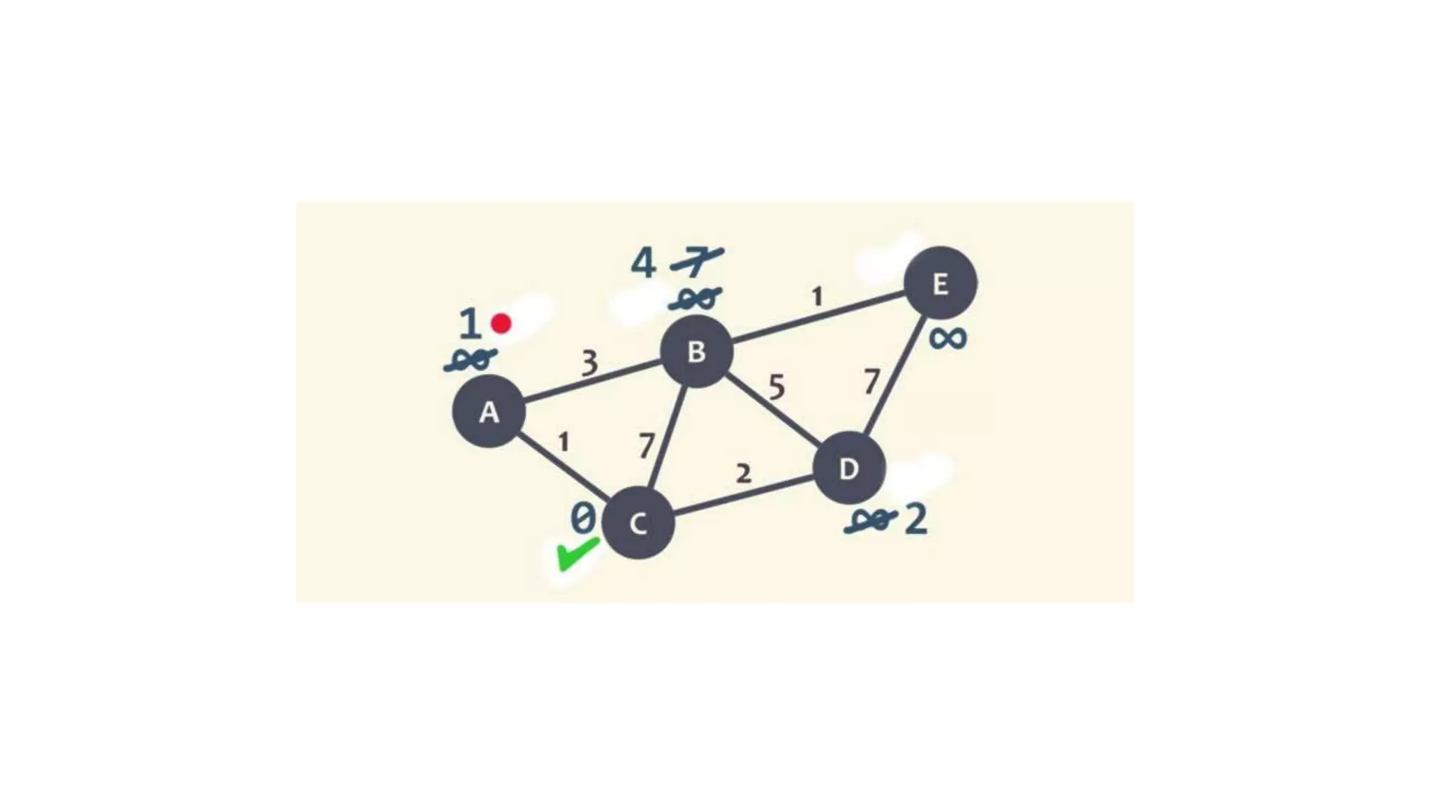
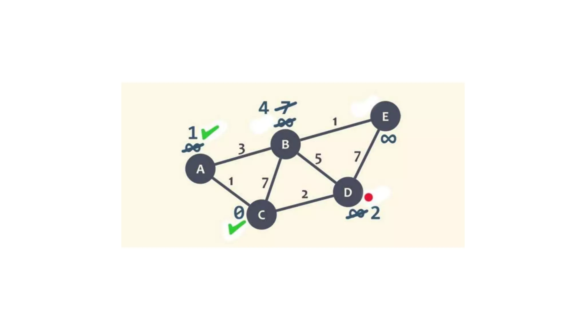
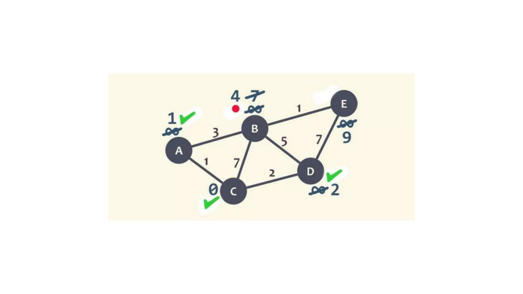
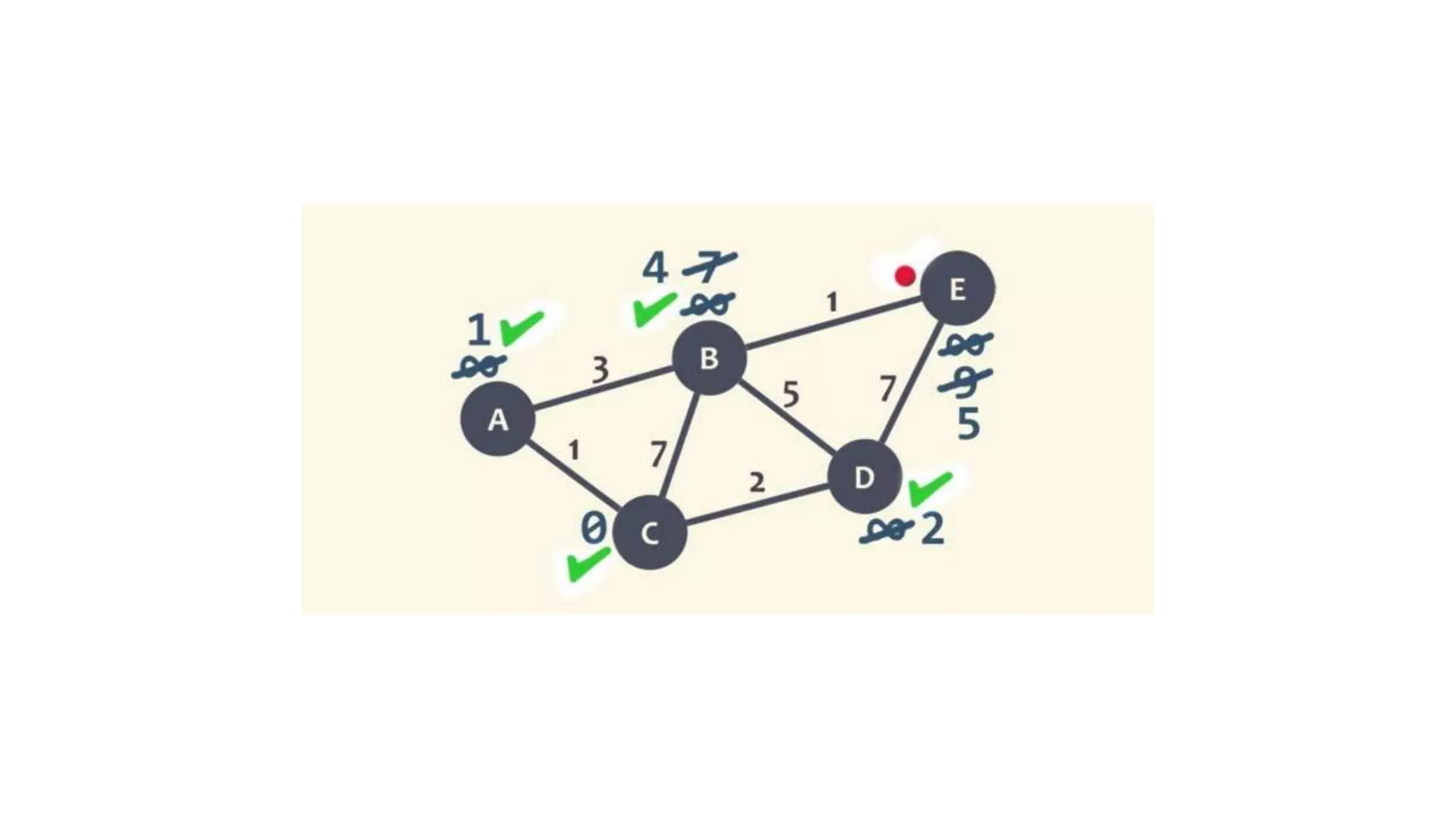
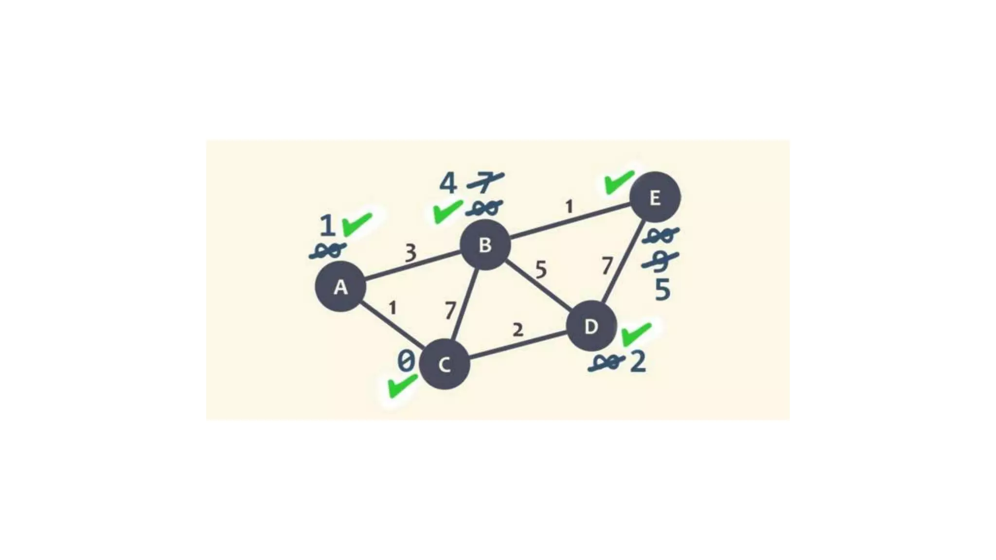
Dijkstra’s
Algorithm
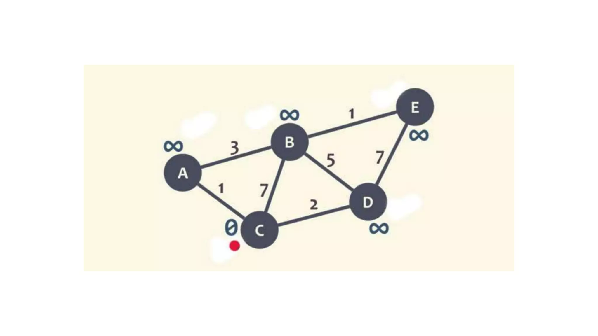
 d[s]  0
 for each v  V – {s}
 do d[v]  
 S  
 Q  V ⊳ Q is a priority queue
maintaining V – S
 while Q  
 do u  EXTRACT-MIN(Q)
 S  S  {u}
 for each v  Adj[u]
 do if d[v] > d[u] + w(u, v)
 then d[v]  d[u] + w(u, v)
p[v]  u
BellmanFord's
Algorithm
 It is similar to Dijkstra's algorithm, but it can work
with graphs in which edges can have negative weights.
 Negative weight edges might seem useless at first, but
they can explain a lot of phenomena like cashflow, the
heat released/absorbed in a chemical reaction, etc.
 For instance, if there are different ways to reach from
one chemical A to another chemical B, each method will
have sub-reactions involving both heat dissipation and
absorption.
 If we want to find the set of reactions where minimum
energy is required, then we will need to be able to
factor in the heat absorption as negative weights and
heat dissipation as positive weights.
237
FloydWarshall
Algorithm
 Floyd Warshall Algorithm is a famous algorithm.
 It is used to solve All Pairs Shortest Path Problem.
 It computes the shortest path between every pair of
vertices of the given graph.
 Floyd Warshall Algorithm is an example of dynamic
programming approach.
 Floyd Warshall Algorithm has the following main
advantages
 It is extremely simple.
 It is easy to implement.
FloydWarshall
Algorithm
 Create a |V| x |V| matrix // It represents the distance between
every pair of vertices as given
 For each cell (i,j) in M do-
 if i = = j
 M[ i ][ j ] = 0 // For all diagonal elements,
value = 0
 if (i , j) is an edge in E
 M[ i ][ j ] = weight(i,j) // If there exists a direct edge
between the vertices, value = weight
 else
 M[ i ][ j ] = infinity // If there is no direct edge
between the vertices, value = ∞
 for k from 1 to |V|
 for i from 1 to |V|
 for j from 1 to |V|
 if M[ i ][ j ] > M[ i ][ k ] + M[ k ][ j ]
 M[ i ][ j ] = M[ i ][ k ] + M[ k ][ j
]
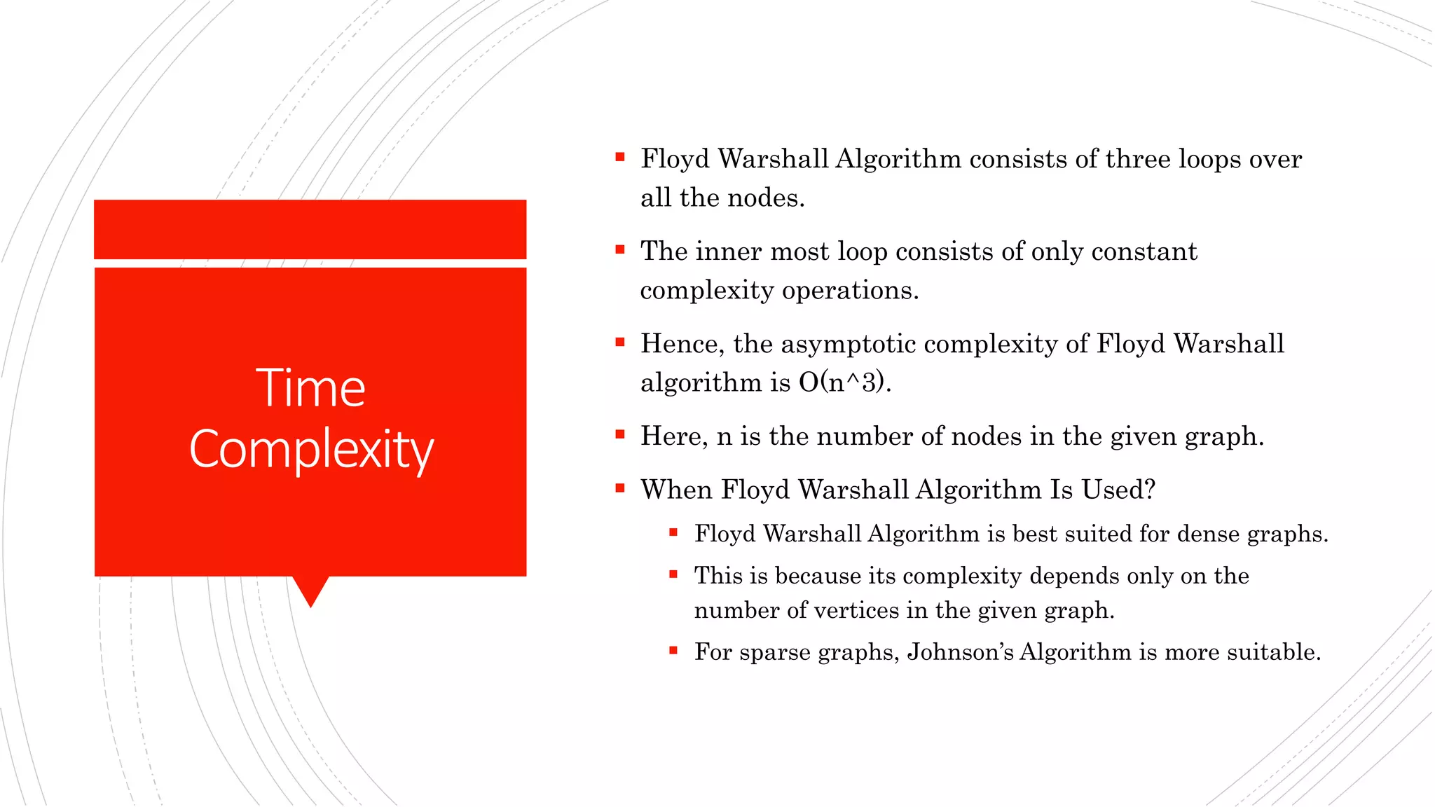
Time
Complexity
 Floyd Warshall Algorithm consists of three loops over
all the nodes.
 The inner most loop consists of only constant
complexity operations.
 Hence, the asymptotic complexity of Floyd Warshall
algorithm is O(n^3).
 Here, n is the number of nodes in the given graph.
 When Floyd Warshall Algorithm Is Used?
 Floyd Warshall Algorithm is best suited for dense graphs.
 This is because its complexity depends only on the
number of vertices in the given graph.
 For sparse graphs, Johnson’s Algorithm is more suitable.
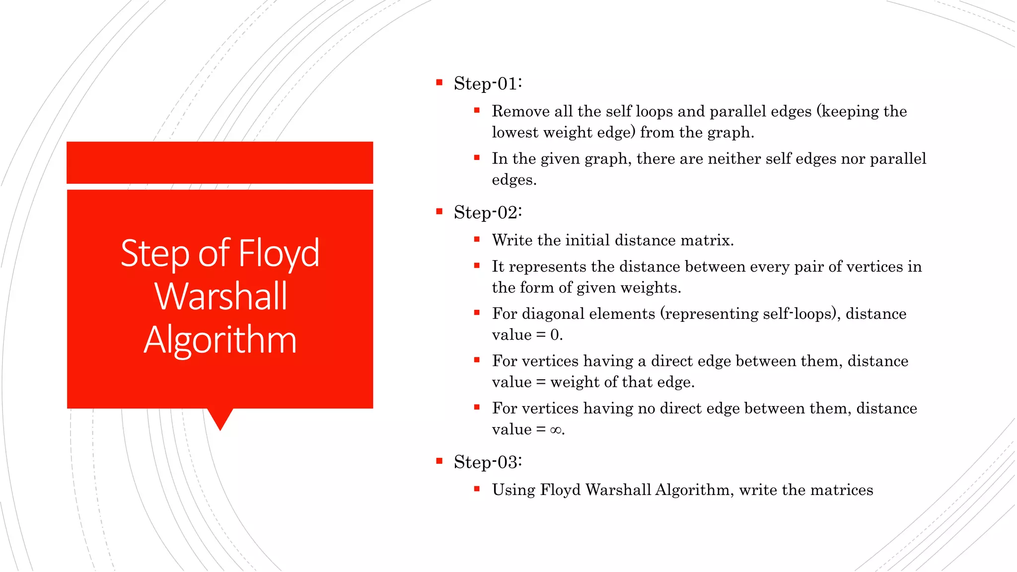
Stepof Floyd
Warshall
Algorithm
 Step-01:
 Remove all the self loops and parallel edges (keeping the
lowest weight edge) from the graph.
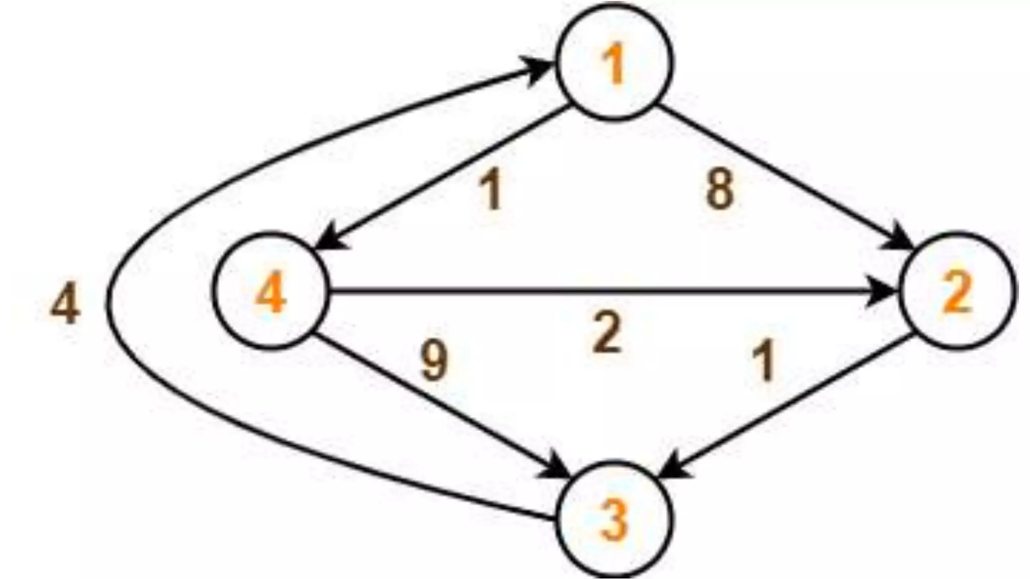
 In the given graph, there are neither self edges nor parallel
edges.
 Step-02:
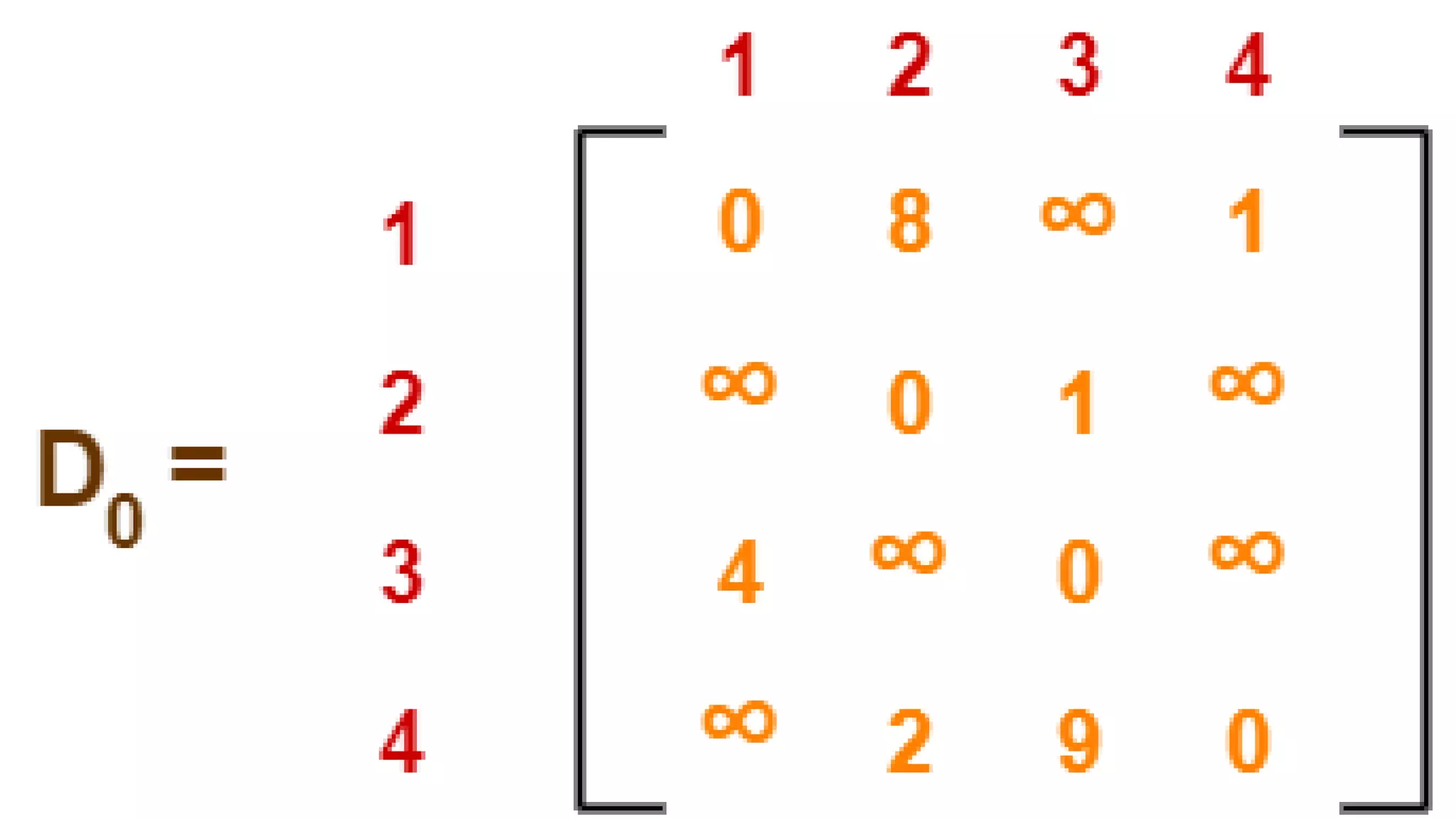
 Write the initial distance matrix.
 It represents the distance between every pair of vertices in
the form of given weights.
 For diagonal elements (representing self-loops), distance
value = 0.
 For vertices having a direct edge between them, distance
value = weight of that edge.
 For vertices having no direct edge between them, distance
value = ∞.
 Step-03:
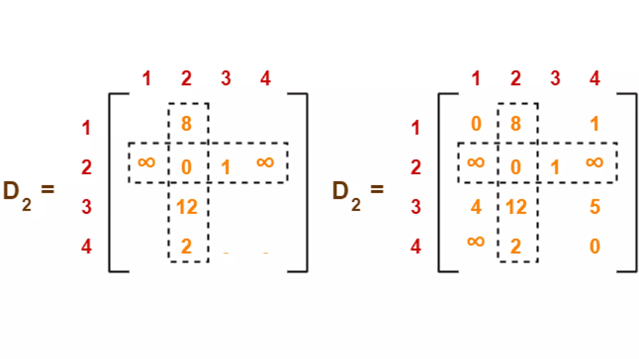
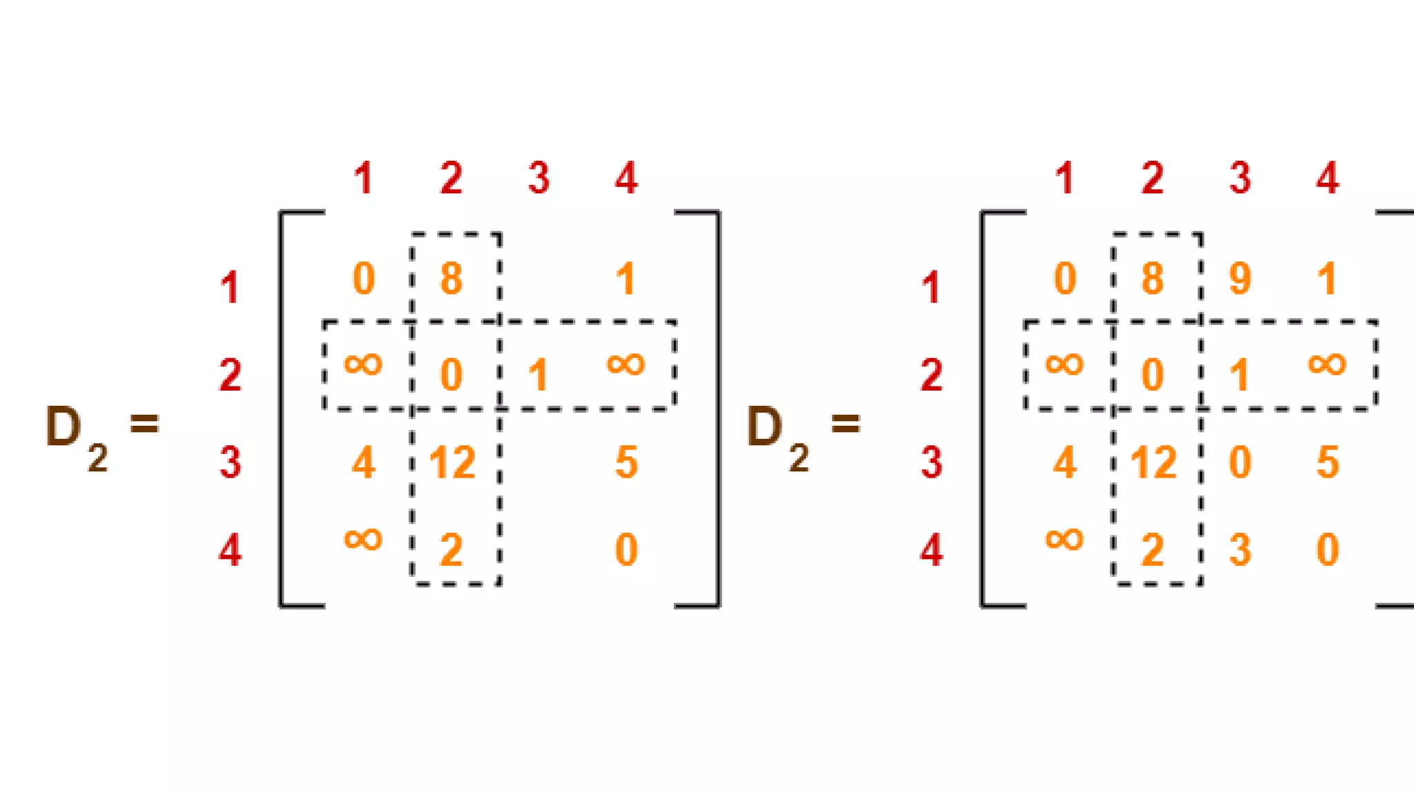
 Using Floyd Warshall Algorithm, write the matrices
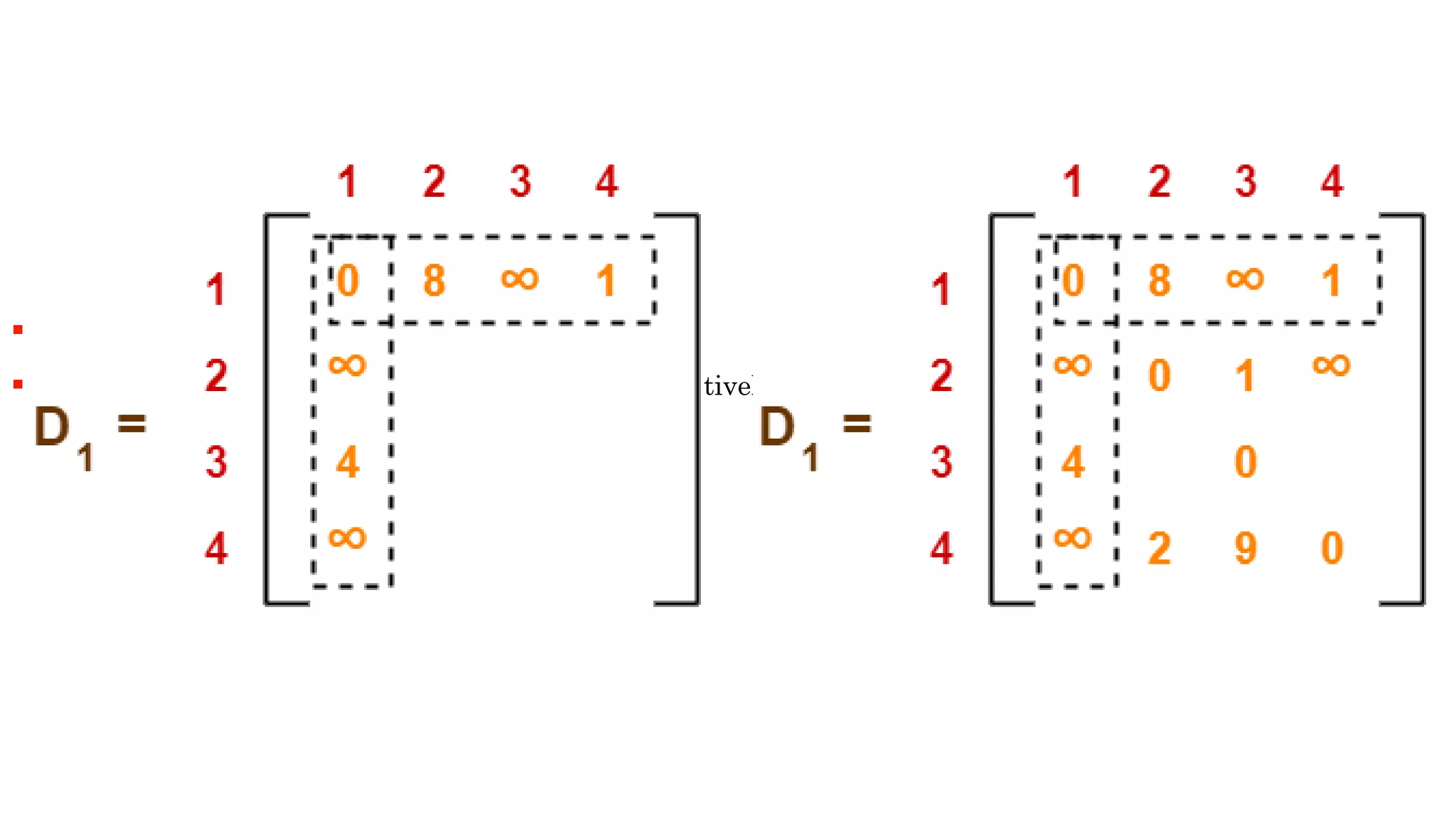
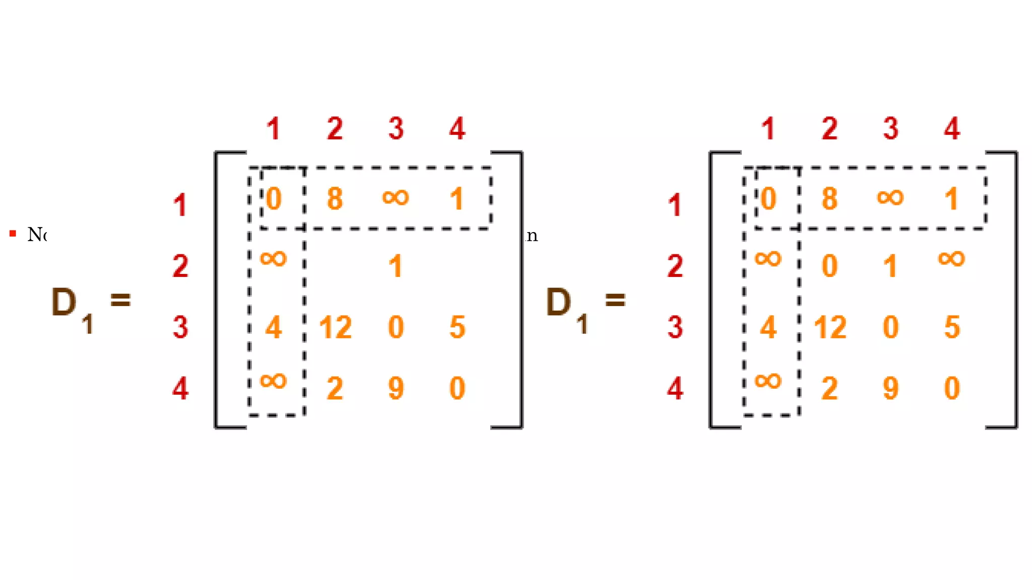
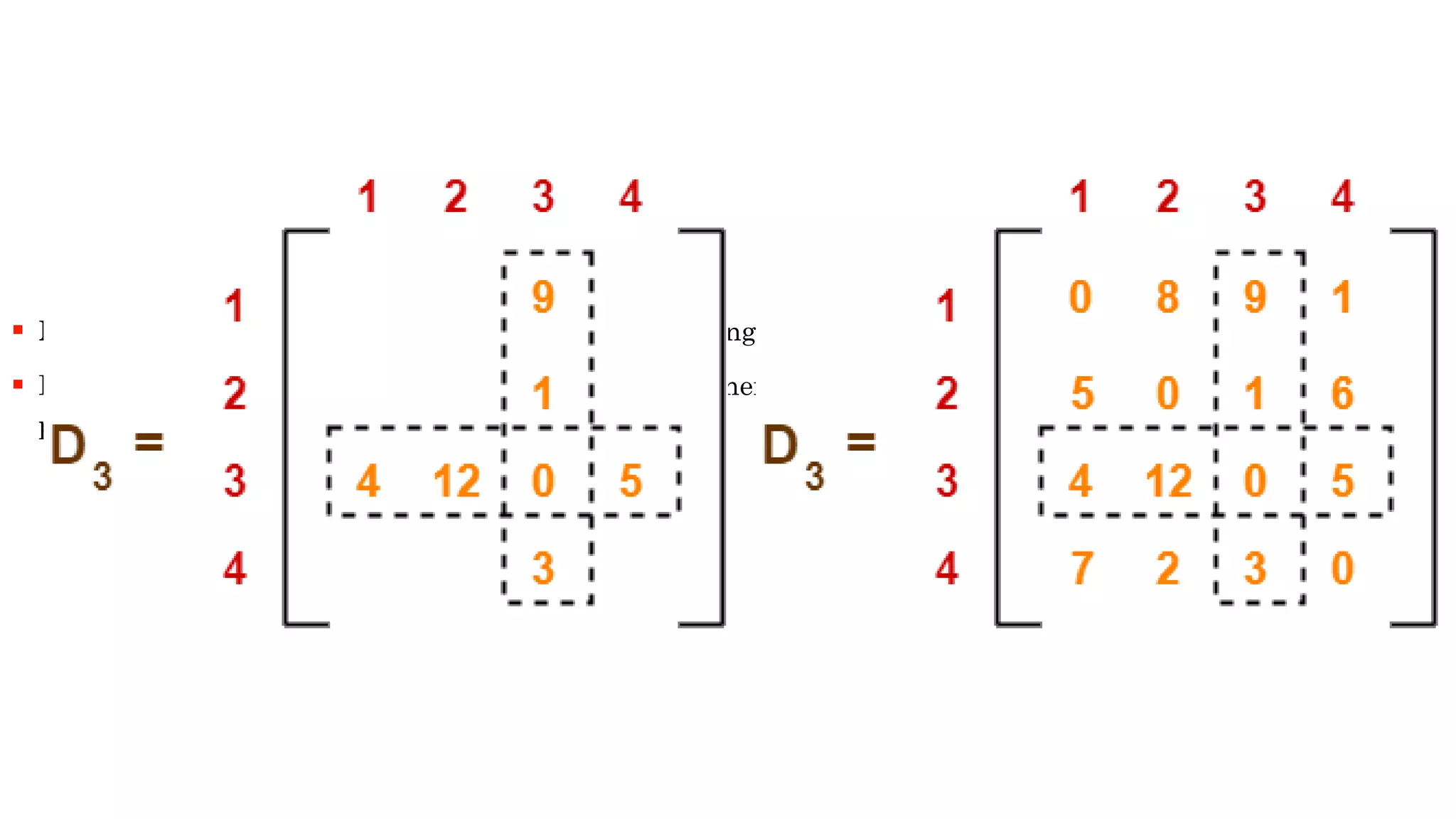
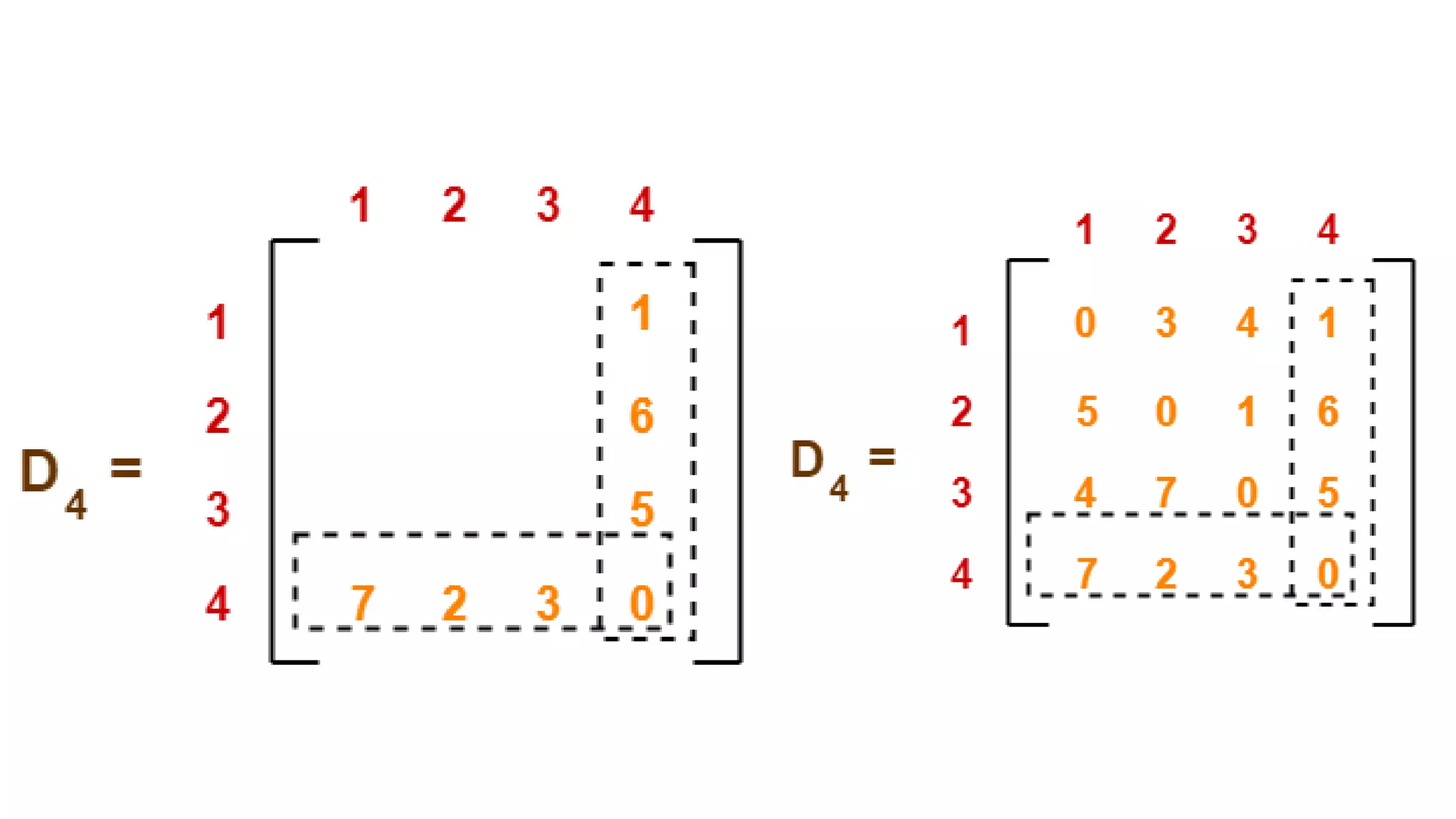
 From D0 put 1 row and column in D1,
 Place infinity rows and column in D1 from D0 respectively
 Now for remaining places add respective row and column value
 Now here we don't have infinity so we add corresponding rows and column value
 If it is smaller than the previous value we replace it otherwise the old value will be
place here
"The best error message
is the one that never
shows up."
Thomas Fuchs
250
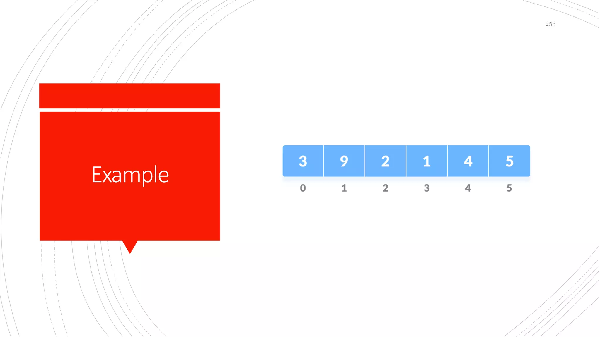
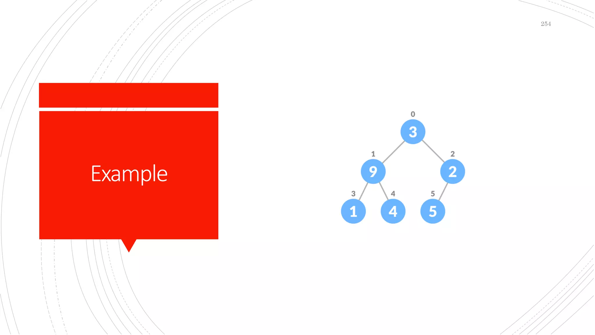
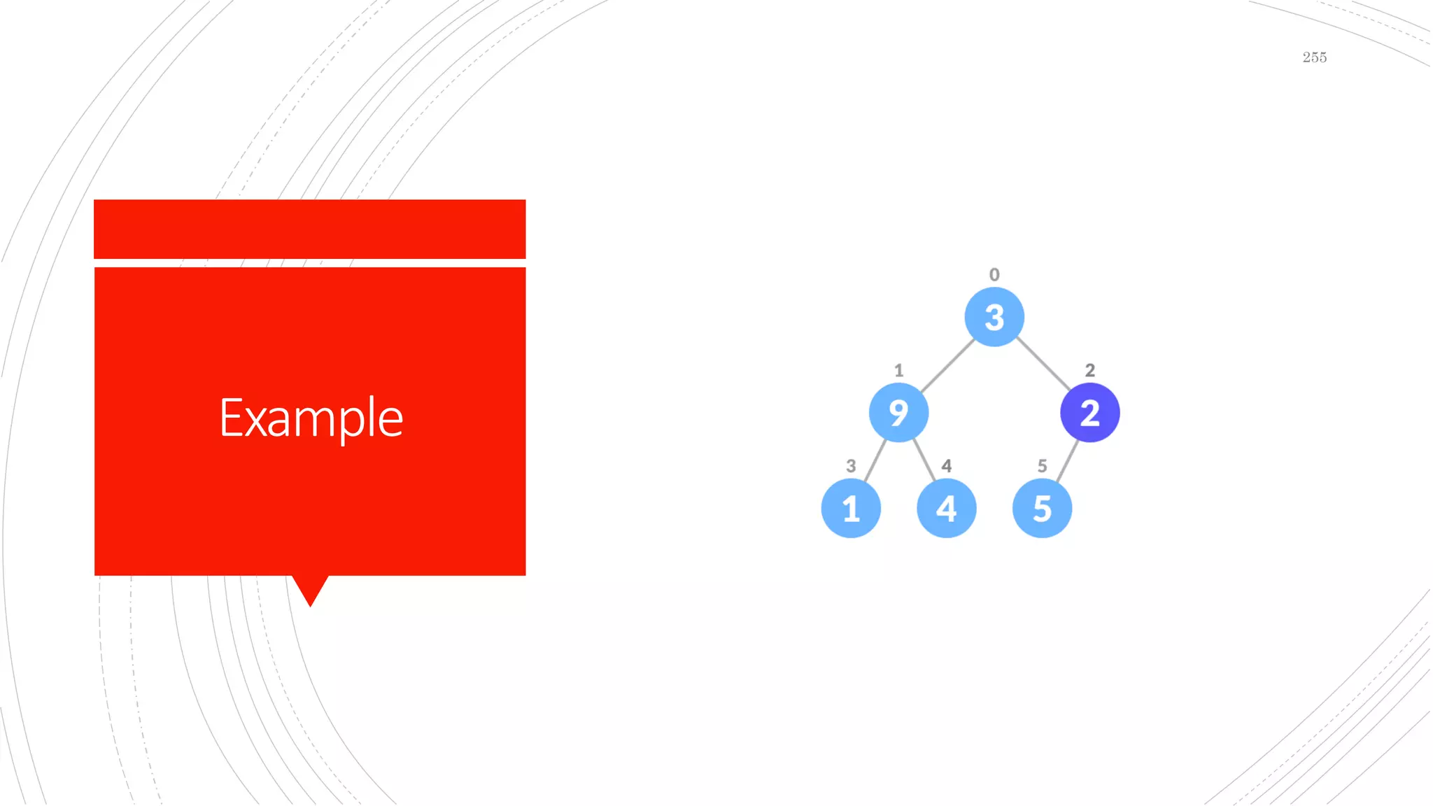
Heap
 Heap data structure is a complete binary tree that
satisfies the heap property, where any given node is
 always greater than its child node/s and the key to the
root node is the largest among all other nodes. This
property is also called max heap property.
 always smaller than the child node/s and the key to the
root node is the smallest among all other nodes. This
property is also called min heap property.
251
Operations
 Heapify
 Heapify is the process of creating a heap data structure
from a binary tree. It is used to create a Min-Heap or a
Max-Heap.
 Insert
 Delete
 Extract Min/Max
252
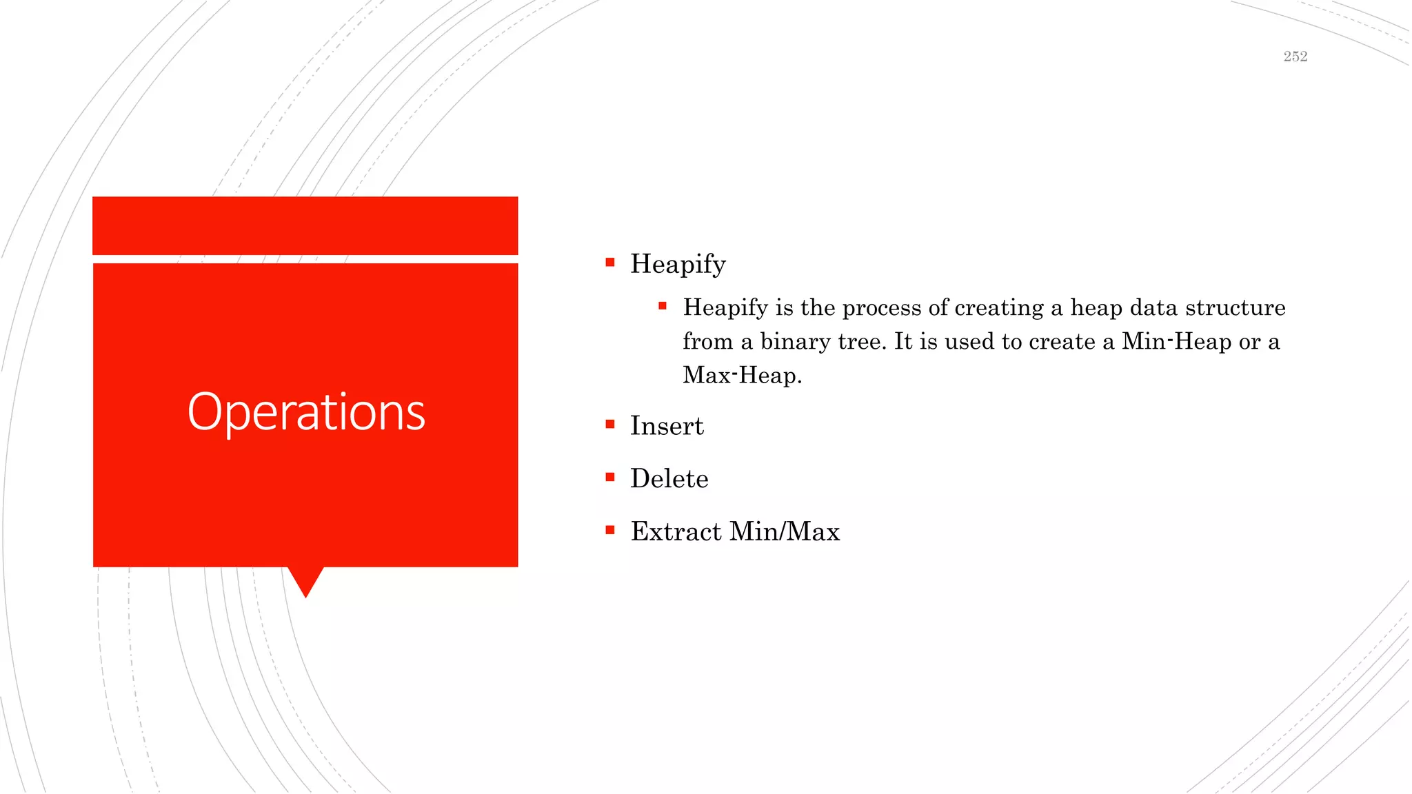
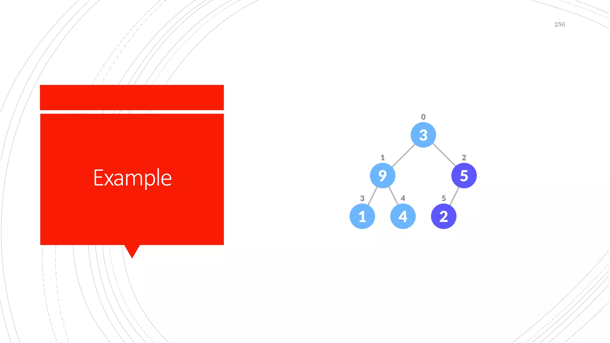
Example
253
Example
254
Example
255
Example
256
HeapSort
 Heap Sort is a popular and efficient sorting algorithm
in computer programming. Learning how to write the
heap sort algorithm requires knowledge of two types of
data structures - arrays and trees.
 The initial set of numbers that we want to sort is
stored in an array e.g. [10, 3, 76, 34, 23, 32] and after
sorting, we get a sorted array [3,10,23,32,34,76].
 Heap sort works by visualizing the elements of the
array as a special kind of complete binary tree called a
heap.
257
Working
 Since the tree satisfies Max-Heap property, then the
largest item is stored at the root node.
 Swap: Remove the root element and put at the end of
the array (nth position) Put the last item of the tree
(heap) at the vacant place.
 Remove: Reduce the size of the heap by 1.
 Heapify: Heapify the root element again so that we
have the highest element at root.
 The process is repeated until all the items of the list
are sorted.
258
“The most damaging
phrase in the language
is.. it's always been
done this way”
Grace Hopper
259
ClassStats
14to 20Feb
 Total Registered Student: 166
 Total Students on portal: 101
 Students at Google Classroom:130
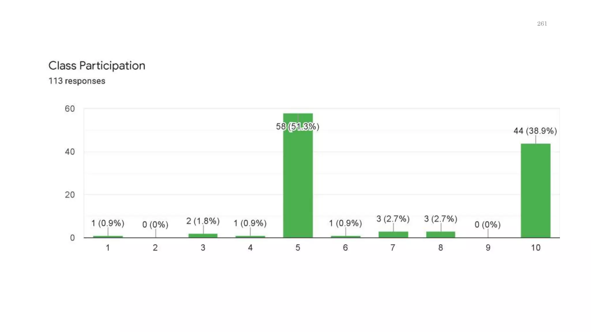
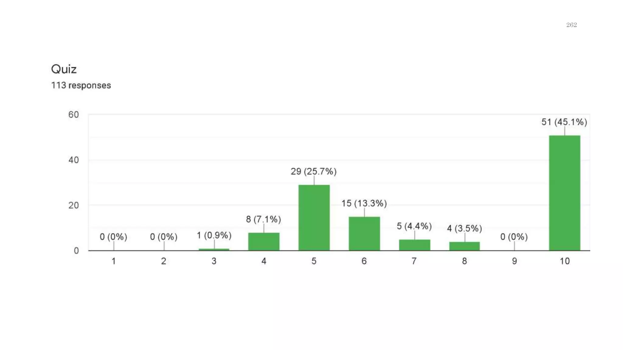
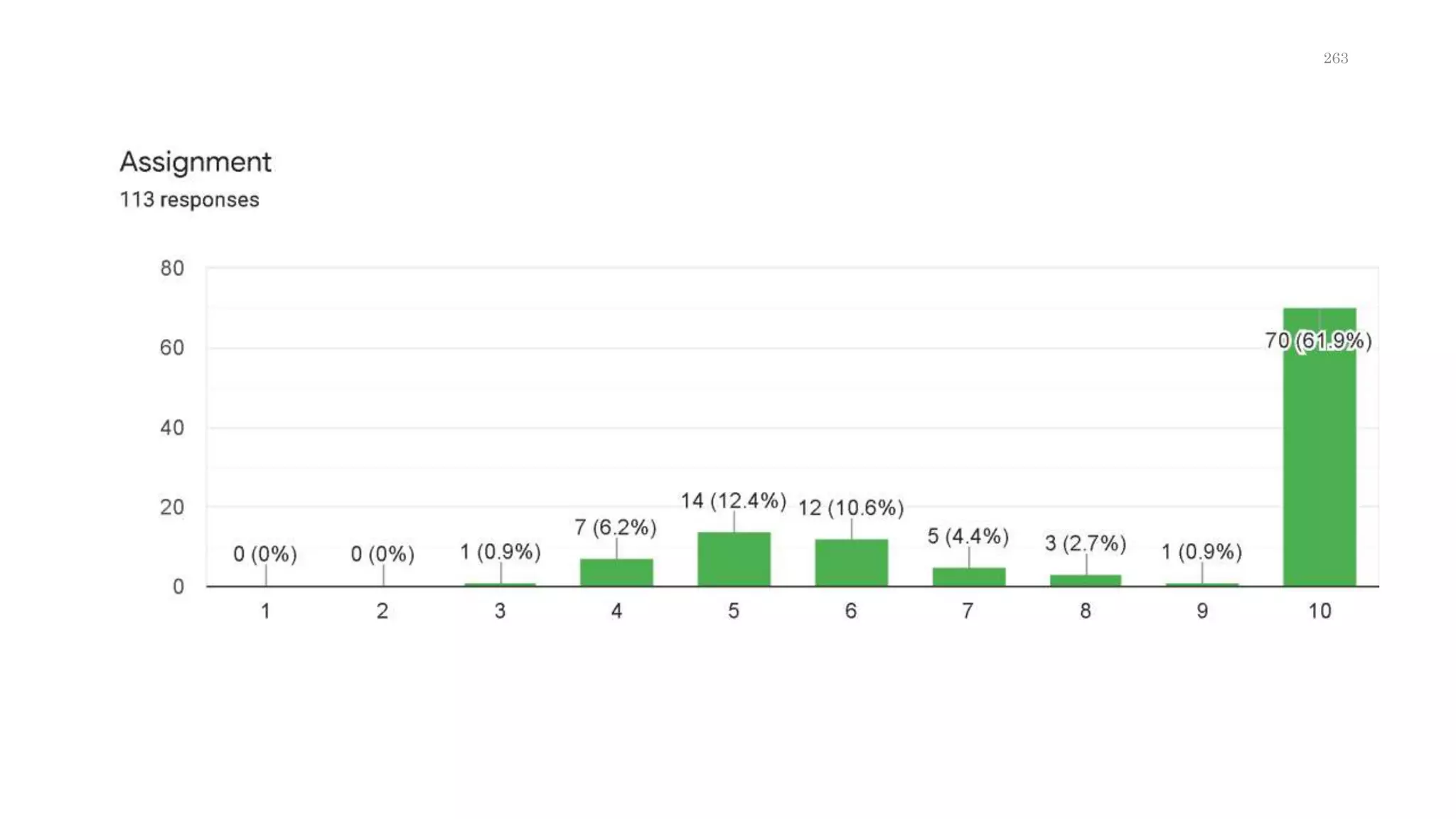
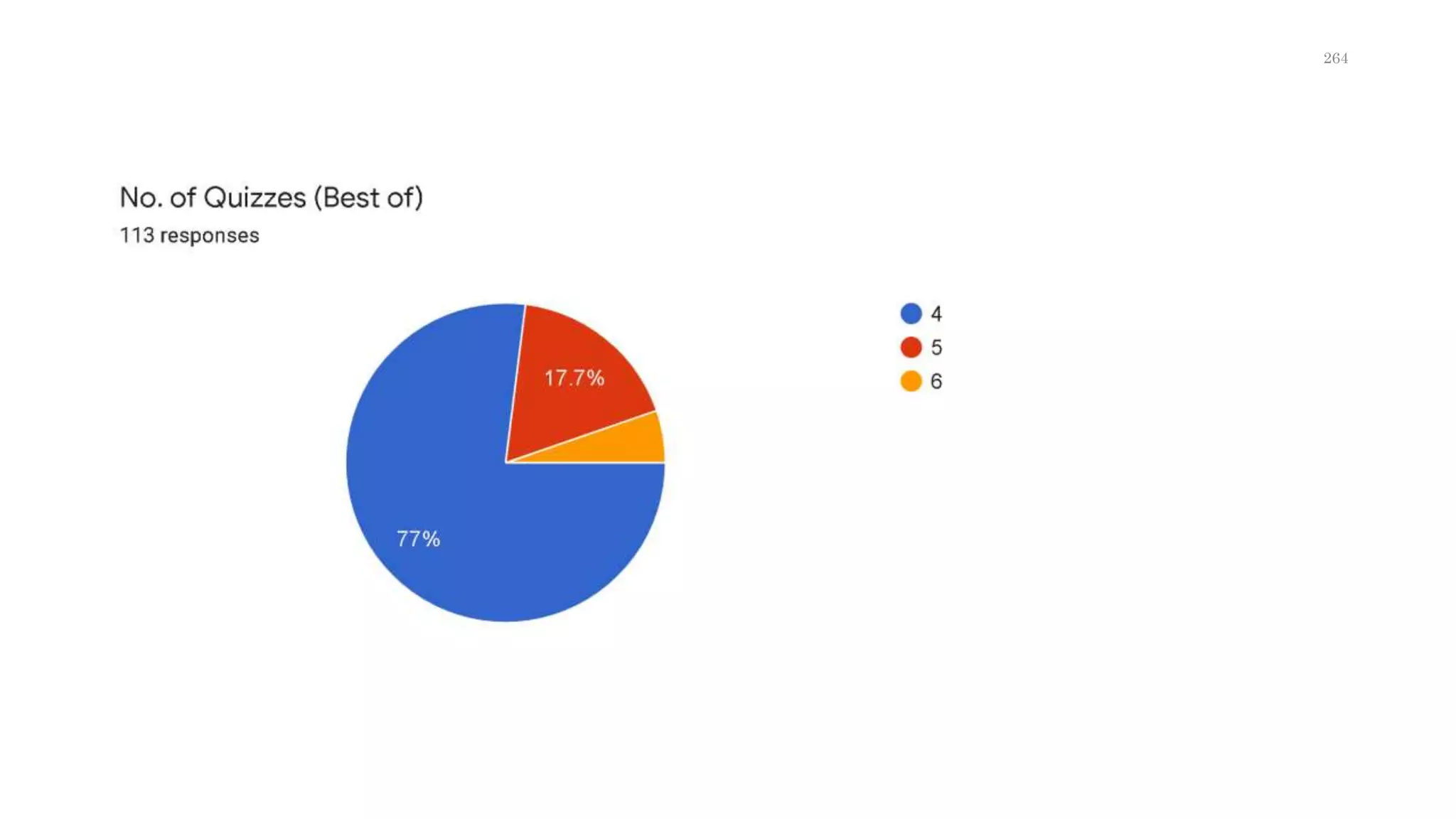
 Class Participation
 Student took part in Marks Distribution:113
260
261
262
263
264
265
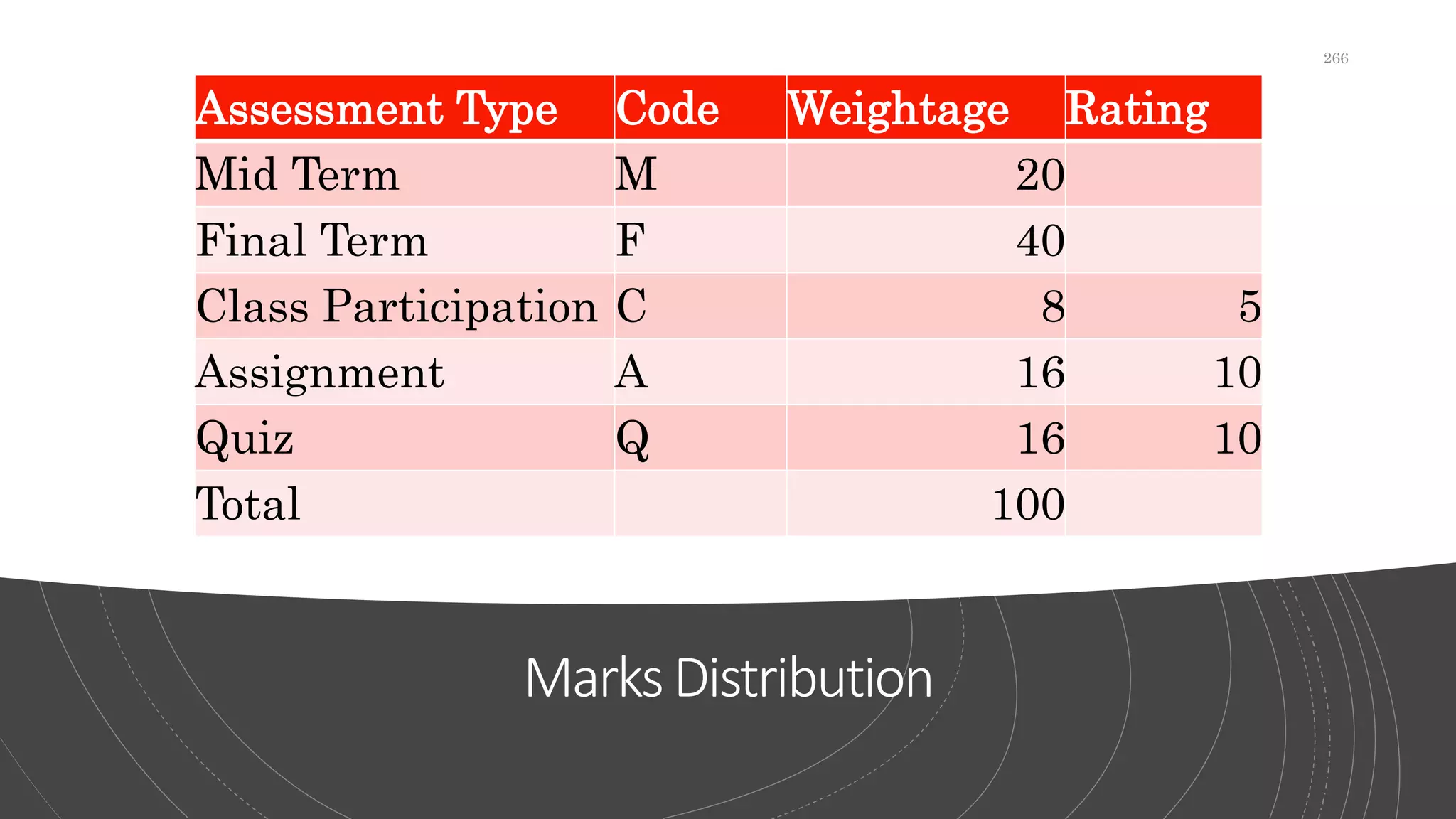
MarksDistribution
Assessment Type Code Weightage Rating
Mid Term M 20
Final Term F 40
Class Participation C 8 5
Assignment A 16 10
Quiz Q 16 10
Total 100
266
ClassParticipation
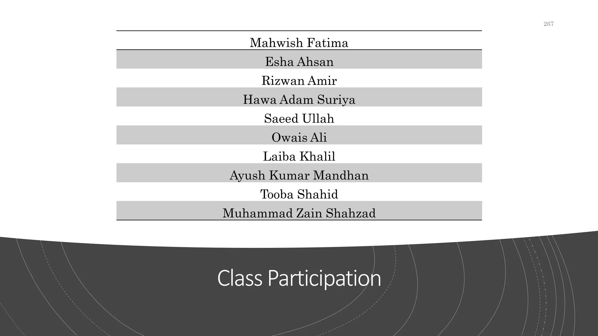
Mahwish Fatima
Esha Ahsan
Rizwan Amir
Hawa Adam Suriya
Saeed Ullah
Owais Ali
Laiba Khalil
Ayush Kumar Mandhan
Tooba Shahid
Muhammad Zain Shahzad
267
Quiz
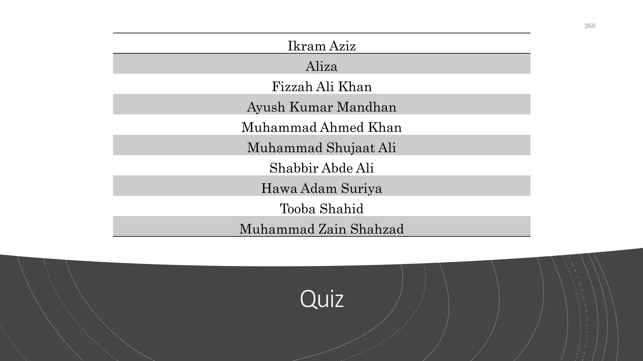
Ikram Aziz
Aliza
Fizzah Ali Khan
Ayush Kumar Mandhan
Muhammad Ahmed Khan
Muhammad Shujaat Ali
Shabbir Abde Ali
Hawa Adam Suriya
Tooba Shahid
Muhammad Zain Shahzad
268
Assignment
Salman Muhammad Syed
Abdul Moiz
Eman
Rizwan Amir
Ayush Kumar Mandhan
Muhammad Ahmed Khan
Muhammad Shujaat Ali
Hawa Adam Suriya
Tooba Shahid
Muhammad Zain Shahzad
269
MidTermPaper
270
Tooba Shahid
Ayush Kumar Mandhan
Muhammad Munim
Esha Ahsan
Umer Ghauri
Kashif Ahmed Khan
Malaika Asad
Eman
Abdul Moiz
Muhammad Ahmed Khan
FinalTerm
271
Top14Students
sp21bsse0001@maju.edu.pk
sp21bsse0057@maju.edu.pk
sp21bscs0052@maju.edu.pk
sp21bscs0043@maju.edu.pk
sp21bscs0031@maju.edu.pk
sp21bscs0039@maju.edu.pk
sp21bscs0056@maju.edu.pk
sp21bscs0032@maju.edu.pk
sp21bsse0026@maju.edu.pk
sp21bscs0076@maju.edu.pk
sp21bscs0074@maju.edu.pk
sp21bsse0005@maju.edu.pk
sp21bscs0087@maju.edu.pk
sp21bsse0034@maju.edu.pk
272

Data Structure and Algorithms.pptx

  • 1.
    “Any fool canwrite code that a computer can understand. Good programmers write code that humans can understand.” Martin Fowler 1
  • 2.
    Data Structure &Algorithms CS-2510 2
  • 3.
    Engr. Syed ZaidIrshad MS Software Engineering (2017) BSc Computer System Engineering (2014) 3
  • 4.
    Rules  No useof Cell Phone (Except Emergency)  Respect Boundaries  Stay Clam and Cool 4
  • 5.
    SubjectMarks Total Marks: 100 MidTerm: 30 Final Term: 40 Class Participation: Quizzes: Max 6, At least 4 Quizzes Assignments: Max 6, At least 4 Assignments 5
  • 6.
    Deadline  Quizzes  OnTime: Obtained Marks  After Due Time: Obtained Marks – 40%  Assignments  Till Due Date: Obtained Marks  After Due Date: Obtained Marks – 40%  Presentation/Quizzes/Assignments  Max Time: May 28, 2022 6
  • 7.
    Outline  Intro toData Structures and Algorithms  Types of data and its nature  DS operations  Time-space trade-off  How to write an algorithm  Introduction to Asymptotic Notation and its importance  Abstract data types arrays  ADT strings and their operations  Introduction to Java  Practical Implementation of Java  Linear Search and Binary Search  Polish notation 7
  • 8.
    Outline  Elementary Sortingtechniques: Bubble, Selection, Insertion  Advance Sorting Techniques: Merge and Quick Sort, Intro to Recursions  Implementing algorithms through recursions  Stacks, its operations, Polish notations  Queues, Types of queues and their representation  Link List (Single Linked List), Traversing, Insertion, Updating and Deletion cases  Doubly Linked List, Traversing, Insertion, updating and deletion cases. Circular Linked List  Sequential Search in Unordered Linked List 8
  • 9.
    Outline  Binary Searchalgorithm with Implementation & Intro to Trees  Binary Search Tree basic  BST implementation, Traversing (BFS, DFS), Insert, update and delete cases  AVL trees Traversing, Insert, update and delete cases  Graph Applications and algorithms, BFS, DFS, SPF graphs  Heap  Hashing Tables  Searching in Strings 9
  • 10.
    Google Classroom Code AM: 3woxzla BM:zwhxaf5 CM: se5a6lk DM: sigjjwh 10
  • 11.
    Your Turn Introduce yourself Name,Why picked this Subject, What you Expect from me (except good marks) 11
  • 12.
    Thinksyou shouldKnow  what isa programming language?  how the instructions can be coded?  how these instructions will be understood by the CPU of computer so that they can be executed?  Choose any language and try to get basics such as  Data types & how memory is allocated to them  Basic arithmetic like add, subtract etc.,  Basic flows such as if, switch , loops etc.  how control flows from one part of a program to another  how to compile & run a program  environments that support this programming language  Basic Discrete Math's: Logic, Probability, Combination, Algebra, Geometry, Topology 12
  • 13.
    Why Learn DSA? To get an output you need two main things:  Data  Procedure  To process the data using procedure you can do:  Smart way  Hard way  If the scope of the problem is big you must consider:  How much Space it need?  How much Time it will take? 13
  • 14.
    Books  Data Structuresand Algorithms in C++ 4th Edition- by Adam Drozdek  Data Structures and algorithms by Goodrich, 4th edition.  Algorithms by Robert and Wayne 4th edition. 14
  • 15.
    DataStructures  Data Structuresare a specialized means of organizing and storing data in computers in such a way that we can perform operations on the stored data more efficiently.  Data structures have a wide and diverse scope of usage across the fields of Computer Science and Software Engineering.  Types  Array  Link List  Stacks  Queues  Hash Tables  Trees  Heaps  Graphs 15
  • 16.
  • 17.
  • 18.
  • 19.
  • 20.
  • 21.
  • 22.
  • 23.
  • 24.
    Operations on Data Structure There are four common operations that can be performed:  Traverse  Search  Insert  Delete 24
  • 25.
    “Before software can bereusable it first has to be usable.” Ralph Johnson 25
  • 26.
    Algorithm  Algorithms area step-by-step equation which makes up a list of actions to perform a task in a program.  Searching: Algorithms are used to search for an item within the data.  Sorting: Algorithms are used to sort different items into a specific order.  Inserting: Algorithms are used to insert items into the data structure.  Updating: Algorithms are used to update items in the data structure.  Deleting: Finally, algorithms can be used to delete items from the data. 26
  • 27.
    Trade-Off  A tradeoffis a situation where one thing increases, and another thing decreases.  It is a way to solve a problem in:  Either in less time and by using more space, or  In very little space by spending a long amount of time, or  Making the right decision depending upon the situation  Types of Space-Time Trade-off  Compressed or Uncompressed data  Re Rendering or Stored images  Smaller code or loop unrolling  Lookup tables or Recalculation 27
  • 28.
    Algorithm Development Process  Step 1:Obtain a description of the problem.  Step 2: Analyze the problem.  Step 3: Develop a high-level algorithm.  Step 4: Refine the algorithm by adding more detail.  Step 5: Review the algorithm. 28
  • 29.
    Obtaina descriptionof theproblem  Defects thatcould be part of the description:  The description relies on unstated assumptions  The description is ambiguous  The description is incomplete  The description has internal contradictions 29
  • 30.
    Analyzethe problem  Starting point What data are available?  Where is that data?  What formulas pertain to the problem?  What rules exist for working with the data?  What relationships exist among the data values?  Ending point  What new facts will we have?  What items will have changed?  What changes will have been made to those items?  What things will no longer exist? 30
  • 31.
    Developahigh- levelalgorithm  Problem: Ineed a send a birthday card to my brother, Mark.  Analysis: I don't have a card. I prefer to buy a card rather than make one myself.  High-level algorithm:  Go to a store that sells greeting cards Select a card Purchase a card Mail the card  This algorithm is satisfactory for daily use, but it lacks details that would have to be added were a computer to carry out the solution. These details include answers to questions such as the following.  "Which store will I visit?"  "How will I get there: walk, drive, ride my bicycle, take the bus?"  "What kind of card does Mark like: humorous, sentimental, risqué?" 31
  • 32.
    Refinethe algorithmby addingmoredetail  A high-levelalgorithm shows the major steps that need to be followed to solve a problem.  Now we need to add details to these steps, but how much detail should we add? Unfortunately, the answer to this question depends on the situation.  We must consider who (or what) is going to implement the algorithm and how much that person (or thing) already knows how to do.  If someone is going to purchase Mark's birthday card on my behalf, my instructions must be adapted to whether that person is familiar with the stores in the community and how well the purchaser knows my brother's taste in greeting cards. 32
  • 33.
    Reviewthe algorithm  Does thisalgorithm solve a very specific problem, or does it solve a more general problem? If it solves a very specific problem, should it be generalized?  Can this algorithm be simplified?  Is this solution like the solution to another problem? How are they alike? How are they different? 33
  • 34.
    Example  A Jeroostarts at (0, 0) facing East with no flowers in its pouch. There is a flower at location (3, 0). Write a program that directs the Jeroo to pick the flower and plant it at a location (3, 2). After planting the flower, the Jeroo should hop one space East and stop. There are no other nets, flowers, or Jeroo's on the island. 34
  • 35.
  • 36.
    Step2  The floweris exactly three spaces ahead of the jeroo.  The flower is to be planted exactly two spaces South of its current location.  The Jeroo is to finish facing East one space East of the planted flower.  There are no nets to worry about. 36
  • 37.
    Step3  Let's namethe Jeroo Bobby. Bobby should do the following:  Get the flower Put the flower Hop East 37
  • 38.
    Step4  Let's namethe Jeroo Bobby. Bobby should do the following:  Get the flower  Hop 3 times Pick the flower  Put the flower  Turn right Hop 2 times Plant a flower  Hop East  Turn left Hop once 38
  • 39.
    Step5  The high-levelalgorithm partitioned the problem into three rather easy subproblems. This seems like a good technique.  This algorithm solves a very specific problem because the Jeroo and the flower are in very specific locations.  This algorithm is a solution to a slightly more general problem in which the Jeroo starts anywhere, and the flower is 3 spaces directly ahead of the Jeroo. 39
  • 40.
    Asymptotic Notations  Asymptotic Notationsare languages that allow us to analyze an algorithm’s running time by identifying its behavior as the input size for the algorithm increases.  These notations invented by Paul Bachmann, Edmund Landau, and others, collectively called Bachmann– Landau notation or asymptotic notation.  This is also known as an algorithm’s growth rate.  Does the algorithm suddenly become incredibly slow when the input size grows?  Does it mostly maintain its quick run time as the input size increases?  Asymptotic Notation gives us the ability to answer these questions. 40
  • 41.
    Functionsof GrowthRates  Constant  1 Logarithmic Function  log n  Linear Function  a*n + b  Quadratic Function  a*n^2 + bn + c  Polynomial Function  a*n^z + . . . + an^2 + a*n^1 + a*n^0  Exponential Function  a^n 41
  • 42.
    Types ofAsymptotic Notations  Big-O notation Omega notation  Theta notation 42
  • 43.
    Big-O  Big Onotation is a mathematical notation that describes the limiting behavior of a function when the argument tends towards a particular value or infinity.  Big-O notation represents the upper bound of the running time of an algorithm. Thus, it gives the worst- case complexity of an algorithm.  f(n) < c*g(n)  For any value of n, the running time of an algorithm does not cross the time provided by O(g(n)). 43
  • 44.
  • 45.
    Stepsto figuring outtheBigO  Step#1: Count the steps  Step #2: Different steps get added  Step#3: Drop constants and coefficients  Step#4: Drop non-dominant terms  Step #5: Different inputs get different variables 45
  • 46.
    Example  Letf(n)=3n4+2n2, find c*g(n) and write in O(g(n)) 46
  • 47.
    Omega notation  Omega notationrepresents the lower bound of the running time of an algorithm.  Thus, it provides the best-case complexity of an algorithm.  f(n)>c*g(n)  For any value of n, the minimum time required by the algorithm is given by Omega Ω(g(n)). 47
  • 48.
  • 49.
    Example  Letf(n)=3n+2, find c*g(n) and write in Ω(g(n)) 49
  • 50.
    Measuring programming progress bythe lines of code is like measuring aircraft building progress by weight. 50
  • 51.
    Theta notation  Thetanotation encloses the function from above and below.  c1*g(n)<f(n)<c2*g(n)  Since it represents the upper and the lower bound of the running time of an algorithm, it is used for analyzing the average-case complexity of an algorithm. 51
  • 52.
  • 53.
    Example Let f(n)=10n3+3n+2, find c1*g(n),c2*g(n) and write in Theta(g(n)) 53
  • 54.
    AbstractData Types  An ADTis a mathematical model of a data structure that specifies the type of data stored, the operations supported on them, and the types of parameters of the operations.  An ADT specifies what each operation does, but not how it does it.  An Abstract Data Type (ADT) is a data type that has values and operations that are not defined in the language itself  Typically, an ADT can be implemented using one of many different data structures.  In Java, an ADT is implemented using a class or an interface 54
  • 55.
    Abstract DataTypes  An AbstractData Type (ADT) consists of:  a set of values  a defined set of properties of these values  a set of operations for processing the values 55
  • 56.
    AbstractData Types  In general,the steps of building ADT to data structures are:  Understand and clarify the nature of the target information unit.  Identify and determine which data objects and operations to include in the models.  Express this property somewhat formally so that it can be understood and communicate well.  Translate this formal specification into proper language. In C++, this becomes a .h file. In Java, this is called "user interface".  Upon finalized specification, write necessary implementation. This includes storage scheme and operational detail. Operational detail is expressed as separate functions (methods). 56
  • 57.
    StringADT  Properties  Thecomponent characters are from the ASCII character set  They are comparable in lexicographic order  They have a length, from 0 to the specified length  Operations on the string ADT include:  Input  Output  Initialization and assignment  Comparison greater, equal, less  Determination of length  Concatenation  Accessing component characters and substrings 57
  • 58.
    Array  Properties:  LinearData Structure  Elements are stored in contiguous memory locations  Can access elements randomly using index  Stores homogeneous elements i.e., similar elements  Syntax:  Array declaration  datatype var_name []=new datatype[size];  datatype[] var_name=new datatype[size];  Can also do declaration and initialization at once  Datatype var_name [] = {ele1, ele2, ele3, ele4}; 58
  • 59.
    Array  Advantages  Randomaccess  Easy sorting and iteration  Replacement of multiple variables  Disadvantages  Size is fixed  Difficult to insert and delete  If capacity is more and occupancy less, most of the array gets wasted  Needs contiguous memory to get allocated  Applications  For storing information in a linear fashion  Suitable for applications that require frequent searching 59
  • 60.
  • 61.
    Demonstration ofArray package array; import java.util.*; publicclass Array { public static void main(String[] args) { int[] priceOfPen= new int[5]; Scanner in=new Scanner(System.in); for(int i=0;i<priceOfPen.length;i++) { System.out.print("Enter pen "+i+" price: "); priceOfPen[i]=in.nextInt(); } for(int i=0;i<priceOfPen.length;i++) System.out.print(priceOfPen[i]+" "); } } 61
  • 62.
    Stack  Properties:  LinearData Structures using Java  Follows LIFO: Last In First Out  Only the top elements are available to be accessed  Insertion and deletion takes place from the top  I.e., a stack of plates, chairs, etc.  Basic Operations of Stack  Push: Add an element to the top of a stack  Pop: Remove an element from the top of a stack  IsEmpty: Check if the stack is empty  IsFull: Check if the stack is full  Peek: Get the value of the top element without removing it 62
  • 63.
    Stack  Advantages  Maintainsdata in a LIFO manner  The last element is readily available for use  All operations are of O(1) complexity  Disadvantages  Manipulation is restricted to the top of the stack  Not much flexible  Applications  Recursion  Parsing  Browser  Editors 63
  • 64.
  • 65.
    Demonstration ofStack (Create) private final intarr[]; private int top; private final int capacity; // Creating a stack Stack(int size) { arr = new int[size]; capacity = size; top = -1; } 65
  • 66.
    Demonstration ofStack (State) // Check ifthe stack is empty public Boolean isEmpty() { return top == -1; } // Check if the stack is full public Boolean isFull() { return top == capacity - 1; } 66
  • 67.
    Demonstration ofStack (Push) // Add elementsinto stack public void push(int x) { if (isFull()) { System.out.println("OverFlownProgram Terminatedn"); System.exit(1); } System.out.println("Inserting " + x); arr[++top] = x; } 67
  • 68.
    Demonstration ofStack (Pop) // Remove elementfrom stack public int pop() { if (isEmpty()) { System.out.println("STACK EMPTY"); System.exit(1); } return arr[top--]; } 68
  • 69.
    Demonstration ofStack (Peek) // Display withoutremoving element from stack public int peek() { if (isEmpty()) { System.out.println("STACK EMPTY"); System.exit(1); } return arr[top]; } 69
  • 70.
    Demonstration ofStack (Print) public void printStack(){ for (int i = 0; i <= top; i++) { System.out.println(arr[i]); } } 70
  • 71.
    Demonstration ofStack (Main) public static voidmain(String[] args) { Stack stack = new Stack(5); stack.push(1); stack.push(2); stack.push(3); stack.push(4); stack.pop(); System.out.println("nAfter popping out"); stack.printStack(); stack.peek(); System.out.println("nAfter peeking"); stack.printStack(); } 71
  • 72.
    PolishNotation  Polish notationis a notation form for expressing arithmetic, logic and algebraic equations.  Its most basic distinguishing feature is that operators are placed on the left of their operands.  If the operator has a defined fixed number of operands, the syntax does not require brackets or parenthesis to lessen ambiguity.  Polish notation is also known as prefix notation, prefix Polish notation, normal Polish notation, Warsaw notation and Lukasiewicz notation. 72
  • 73.
    Types  Infix Notation We write expression in infix notation, e.g., a - b + c  Prefix Notation  In this notation, operator is prefixed to operands, i.e. operator is written ahead of operands. For example, +ab. This is equivalent to its infix notation a + b. Prefix notation is also known as Polish Notation.  Postfix Notation  This notation style is known as Reversed Polish Notation. In this notation style, the operator is postfixed to the operands i.e., the operator is written after the operands. For example, ab+. This is equivalent to its infix notation a + b. 73
  • 74.
    PostfixNotation  Step 1:Add '')" to the end of the infix expression  Step 2: Push ( onto the stack  Step 3: Repeat until each character in the infix notation is scanned  IF a ( is encountered, push it on the stack  IF an operand (whether a digit or a character) is encountered, add it postfix expression.  IF a ")" is encountered, then a. Repeatedly pop from stack and add it to the postfix expression until a "(" is encountered. b. Discard the "(".That is, remove the(from stack and do not add it to the postfix expression  IF an operator O is encountered, then a. Repeatedly pop from stack and add each operator ( popped from the stack) to the postfix expression which has the same precedence or a higher precedence than O b. Push the operator to the stack  [END OF IF]  Step 4: Repeatedly pop from the stack and add it to the postfix expression until the stack is empty  Step 5: EXIT 74
  • 75.
    Without requirements or design,programming is the art of adding bugs to an empty text file. 75
  • 76.
    PrefixNotation  Step 1:Reverse the infix string. Note that while reversing the string you must interchange left and right parentheses.  Step 2: Obtain the postfix expression of the infix expression Step 1.  Step 3: Reverse the postfix expression to get the prefix expression 76
  • 77.
    Examples S.No. Infix Notation Prefix Notation Postfix Notation 1a + b 2 (a + b) ∗ c 3 a ∗ (b + c) 4 a / b + c / d 5 (a + b) ∗ (c + d) 6 ((a + b) ∗ c) - d 77
  • 78.
    Examples S.No. Infix Notation Prefix Notation Postfix Notation 1a + b + a b a b + 2 (a + b) ∗ c ∗ + a b c a b + c ∗ 3 a ∗ (b + c) ∗ a + b c a b c + ∗ 4 a / b + c / d + / a b / c d a b / c d / + 5 (a + b) ∗ (c + d) ∗ + a b + c d a b + c d + ∗ 6 ((a + b) ∗ c) - d - ∗ + a b c d a b + c ∗ d - 78
  • 79.
    Example 5 *( ( ( 9 + 8 ) + ( 4 * 6 ) ) - 7 ) 79
  • 80.
    Step by Step Conversion 5* ( ( ( 9 + 8 ) + ( 4 * 6 ) ) - 7 ) Expression Stack Postfix 5 5 * * 5 9 *((( 59 + *(((+ 59 8 *(((+ 598 ) *(( 598+ + *((+ 598+ 4 *((+( 598+4 * *((+(* 598+4 6 *((+(* 598+46 ) *((+ 598+46* 80
  • 81.
    Step by Step Conversion 5* ( ( ( 9 + 8 ) + ( 4 * 6 ) ) - 7 ) Expression Stack Postfix ) *( 598+46*+ - *(- 598+46*+ 7 *(- 598+46*+7 ) * 598+46*+7- 598+46*+7-* 81
  • 82.
    Post/Pre-fix Postfix :598+46*+7-* | Prefix : *5-++98*467 82
  • 83.
    Example  Postfix form: 5 9 8 + 4 6 * + 7 - *  Push( 5 ) Push( 9 ) Push( 8 )  Push( Pop() + Pop() )  Push( 4 ) Push( 6 )  Push( Pop() * Pop() )  Push( Pop() + Pop() )  Push( 7 )  Push( Pop() - Pop() )  Push( Pop() * Pop() )  Answer: 170 83
  • 84.
    Queue  Properties  LinearData Structure  Follows FIFO: First In First Out  Insertion can take place from the rear end.  Deletion can take place from the front end.  E.g.: queue at ticket counters, bus station  5 major operations:  Enqueue: Add an element to the end of the queue  Dequeue: Remove an element from the front of the queue  IsEmpty: Check if the queue is empty  IsFull: Check if the queue is full  Peek: Get the value of the front of the queue without removing it 84
  • 85.
    Queue  Advantages  Maintainsdata in FIFO manner  Insertion from beginning and deletion from end takes O(1) time  Applications  Scheduling  Maintaining playlist  Interrupt handling 85
  • 86.
  • 87.
    Demonstration ofQueue (Create) int SIZE =5; int items[] = new int[SIZE]; int front, rear; Queue() { front = -1; rear = -1; } 87
  • 88.
    Demonstration ofQueue (State) boolean isFull() { if(front == 0 && rear == SIZE - 1) { return true; } return false; } boolean isEmpty() { if (front == -1) return true; else return false; } 88
  • 89.
    Demonstration ofQueue (Enqueue) void enQueue(int element){ if (isFull()) { System.out.println("Queue is full"); } else { if (front == -1) front = 0; rear++; items[rear] = element; System.out.println("Inserted " + element); } } 89
  • 90.
    Demonstration ofQueue (Dequeue) if (isEmpty()) { System.out.println("Queueis empty"); return (-1); } else { element = items[front]; if (front >= rear) { front = -1; rear = -1; } else { front++; } System.out.println("Deleted -> " + element); return (element); 90
  • 91.
  • 92.
    Typesof Queue  Thereare four different types of queues:  Simple Queue  Circular Queue  Priority Queue  Double Ended Queue 92
  • 93.
  • 94.
  • 95.
  • 96.
  • 97.
  • 98.
  • 99.
    Demonstration ofQueue (State) if (front ==0 && rear == SIZE - 1) { return true; } if (front == rear + 1) { return true; } return false; } // Check if the queue is empty boolean isEmpty() { if (front == -1) return true; else return false; 99
  • 100.
    "Programming isn't about whatyou know; it's about what you can figure out.” Chris Pine 100
  • 101.
    Demonstration ofQueue (Enqueue) void enQueue(int element){ if (isFull()) { System.out.println("Queue is full"); } else { if (front == -1) front = 0; rear = (rear + 1) % SIZE; items[rear] = element; System.out.println("Inserted " + element); } } 101
  • 102.
    Demonstration ofQueue (Dequeue) int element; if (isEmpty()){ System.out.println("Queue is empty"); return (-1); } else { element = items[front]; if (front == rear) { front = -1; rear = -1; } else { front = (front + 1) % SIZE; } return (element); } 102
  • 103.
    PriorityQueue  Types ofPriority Queue:  Min Priority Queue: In min priority Queue minimum number of value gets the highest priority and lowest number of element gets the highest priority.  Max Priority Queue: Max priority Queue is where maximum number value gets the highest priority and minimum number of value gets the minimum priority. 103
  • 104.
    Demonstration ofPQueue (Dequeue) int deQueue() { …..... inti, max = 0; // find the maximum priority for (i = 1; i < n; i++) { if (items[max] < items[i]) { max = i; } } element = items[max]; …..... queue[max] = queue[rear - 1]; rear = rear - 1; 104
  • 105.
    Deque  Types ofDeque  Input Restricted Deque: In this deque, input is restricted at a single end but allows deletion at both the ends.  Output Restricted Deque: In this deque, output is restricted at a single end but allows insertion at both the ends. 105
  • 106.
    Demonstration ofDeque (State)  boolean isFull(){  return ((front == 0 && rear == size - 1) || front == rear + 1);  }   boolean isEmpty() {  return (front == -1);  } 106
  • 107.
    Demonstration ofDeque (EnqueueFront) void insertfront(int key){ if (isFull()) { System.out.println("Overflow"); return; } if (front == -1) { front = 0; rear = 0; } else if (front == 0) front = size - 1; else front = front - 1; arr[front] = key; } 107
  • 108.
    Demonstration ofDeque (EnqueueRear) void insertrear(int key){ if (isFull()) { System.out.println(" Overflow "); return; } if (front == -1) { front = 0; rear = 0; } else if (rear == size - 1) rear = 0; else rear = rear + 1; arr[rear] = key; } 108
  • 109.
    Demonstration ofDeque (DequeueFront) if (isEmpty()) { System.out.println("Queue Underflown"); return; } //Deque has only one element if (front == rear) { front = -1; rear = -1; } else if (front == size - 1) front = 0; else front = front + 1; 109
  • 110.
    Demonstration ofDeque (DequeueRear) void deleterear() { if(isEmpty()) { System.out.println(" Underflow"); return; } if (front == rear) { front = -1; rear = -1; } else if (rear == 0) rear = size - 1; else rear = rear - 1; } 110
  • 111.
    Linkedlist  Properties  LinearData Structure  Elements can be stored as per memory availability  Can access elements on linear fashion only  Stores homogeneous elements i.e., similar elements  Dynamic in size  Easy insertion and deletion  Starting element or Node is the key which is generally termed as head.  There are three common types of Linked List.  Singly Linked List  Doubly Linked List  Circular Linked List 111
  • 112.
    LinkedList  Advantages  Dynamicin size  No wastage as capacity and size is always equal  Easy insertion and deletion as 1 link manipulation is required  Efficient memory allocation  Disadvantages  If head Node is lost, the linked list is lost  No random access possible  Applications  Suitable where memory is limited  Suitable for applications that require frequent insertion and deletion 112
  • 113.
    Demonstration ofLinked List(Create) class LinkedList { //Creating a node Node head; static class Node { int value; Node next; Node(int d) { value = d; next = null; } } 113
  • 114.
    Demonstrationof LinkedList(Main) // Assign valuevalues linkedList.head = new Node(1); Node second = new Node(2); Node third = new Node(3); // Connect nodess linkedList.head.next = second; second.next = third; // printing node-value while (linkedList.head != null) { System.out.print(linkedList.head.value + " "); linkedList.head = linkedList.head.next; 114
  • 115.
    Demonstrationof LinkedList (InsertBeginning) // Insert atthe beginning public void insertAtBeginning(int new_data) { // insert the data Node new_node = new Node(new_data); new_node.next = head; head = new_node; } 115
  • 116.
    Demonstration ofLinkedList (InsertEnd) Node new_node =new Node(new_data); if (head == null) { head = new Node(new_data); return; } new_node.next = null; Node last = head; while (last.next != null) last = last.next; last.next = new_node; 116
  • 117.
    Demonstrationof LinkedList (InsertAnypoint) // Insert aftera node public void insertAfter(Node prev_node, int new_data) { if (prev_node == null) { System.out.println("The given previous node cannot be null"); return; } Node new_node = new Node(new_data); new_node.next = prev_node.next; prev_node.next = new_node; } 117
  • 118.
    Demonstration ofLinkedList (Delete) return; Node temp =head; if (position == 0) { head = temp.next; return; } // Find the key to be deleted for (int i = 0; temp != null && i < position - 1; i++) temp = temp.next; // If the key is not present if (temp == null || temp.next == null) return; // Remove the node Node next = temp.next.next; 118
  • 119.
    Demonstration ofLinkedList (Display) // Print thelinked list public void printList() { Node tnode = head; while (tnode != null) { System.out.print(tnode.data + " "); tnode = tnode.next; } } 119
  • 120.
    Demonstration ofDoublyLinked List(Create) public class DoublyLinkedList{ // node creation Node head; class Node { int data; Node prev; Node next; Node(int d) { data = d; } } 120
  • 121.
    Demonstrationof DoublyLinkedList (Main) DoublyLinkedList doubly_ll =new DoublyLinkedList(); doubly_ll.insertEnd(5); doubly_ll.insertFront(1); doubly_ll.insertFront(6); doubly_ll.insertEnd(9); // insert 11 after head doubly_ll.insertAfter(doubly_ll.head, 11); // insert 15 after the seond node doubly_ll.insertAfter(doubly_ll.head.next, 11); doubly_ll.printlist(doubly_ll.head); // delete the last node doubly_ll.deleteNode(doubly_ll.head.next.next.next.next.next); doubly_ll.printlist(doubly_ll.head); 121
  • 122.
    Demonstrationof DoubleLinkedList (InsertBeginning) public void insertFront(intdata) { // allocate memory for newNode and assign data to newNode Node newNode = new Node(data); // make newNode as a head newNode.next = head; // assign null to prev of newNode newNode.prev = null; // previous of head (now head is the second node) is newNode if (head != null) head.prev = newNode; // head points to newNode head = newNode; } 122
  • 123.
    Demonstrationof DoublyLinkedList (InsertEnd) // insert anewNode at the end of the list void insertEnd(int data) { // allocate memory for newNode and assign data to newNode Node new_node = new Node(data); // store the head node temporarily (for later use) Node temp = head; // assign null to next of newNode new_node.next = null; // if the linked list is empty, make the newNode as head node if (head == null) { new_node.prev = null; head = new_node; return; } 123
  • 124.
    Demonstrationof DoubleLinked List (AnyPoint) // insert anode after a specific node public void insertAfter(Node prev_node, int data) { // check if previous node is null if (prev_node == null) { System.out.println("previous node cannot be null"); return; } // allocate memory for newNode and assign data to newNode Node new_node = new Node(data); // set next of newNode to next of prev node new_node.next = prev_node.next; // set next of prev node to newNode prev_node.next = new_node; // set prev of newNode to the previous node new_node.prev = prev_node; // set prev of newNode's next to newNode if (new_node.next != null) new_node.next.prev = new_node; } 124
  • 125.
    "The only wayto learn a new programming language is by writing programs in it." Dennis Ritchie 125
  • 126.
    CircularLinkList  Connect Lastto Head by storing value of Head in Last's node next 126
  • 127.
    Sortingand Searching  Storing andretrieving information is one of the most common application of computers now-a-days.  According to time the amount of data and information stored and accessed via computer has turned to huge databases.  So many techniques and algorithms have been developed to efficiently maintain and process information in databases.  The processes of looking up a particular data record in the database is called searching.  The process of ordering the records in a database is called Sorting.  Sorting and searching together constitute a major area of study in computational methods. 127
  • 128.
    Search  Searching isthe process of finding a particular item in a collection of items.  A search typically answers whether the item is present in the collection or not.  When the key field of a target item is found, a pointer to the target item is returned.  The pointer may be an address, an index into a vector or array, or some other indication of where to find the target.  If a matching key field isn’t found, the user is informed. 128
  • 129.
  • 130.
    LinearSearch Step 1: Seti to 1 Step 2: if i > n then go to step 7 Step 3: if A[i] = x then go to step 6 Step 4: Set i to i + 1 Step 5: Go to Step 2 Step 6: Print Element x Found at index i and go to step 8 Step 7: Print element not found 130
  • 131.
    JavaCode class LinearSearch { publicstatic int linearSearch(int array[], int x) { int n = array.length; // Going through array sequencially for (int i = 0; i < n; i++) { if (array[i] == x) return i; } return -1; } public static void main(String args[]) { int array[] = { 2, 4, 0, 1, 9 }; int x = 1; int result = linearSearch(array, x); if (result == -1) System.out.print("Element not found"); else System.out.print("Element found at index: " + result); } } 131
  • 132.
    BinarySearch Step 1: Datalist must be ordered list in ascending order. Step 2: Probe middle of list Step 3: If target equals list[mid], FOUND. Step 4: If target < list[mid], discard 1/2 of list between list[mid] and list[last]. Step 5: If target > list[mid], discard 1/2 of list between list[first] and list[mid]. Step 6: Continue searching the shortened list until either the target is found, or there are no elements to probe. 132
  • 133.
    JavaCode while (low <=high) { int mid = low + (high - low) / 2; if (array[mid] == x) return mid; if (array[mid] < x) low = mid + 1; else high = mid - 1; } return -1; } public static void main(String args[]) { BinarySearch ob = new BinarySearch(); int array[] = { 3, 4, 5, 6, 7, 8, 9 }; int n = array.length; int x = 4; int result = ob.binarySearch(array, x, 0, n - 1); if (result == -1) System.out.println("Not found"); else 133
  • 134.
    Analysis Linear Binary Big-O O(n)O(log n) Omega O(1) O(1) 134
  • 135.
    Sort  Sorting isthe process of placing elements from a collection in order.  For example, a list of words could be sorted alphabetically or by length.  Efficient sorting is important to optimize the use of other algorithms that require sorted lists to work correctly.  There are two main types of Sort:  Internal (Sort happens in primary memory)  External (Sort happens in primary + secondary memory) 135
  • 136.
    CommonSortingAlgorithms •Bubble Sort •Insertion Sort •SelectionSort •Quick Sort Internal Sort •Merge Sort External Sort 136
  • 137.
    Bubble set swap flagto false for j=1 to i { if list[j-1] > list[j] swap list[j-1] and list[j] set swap flag to true } if swap flag is false, break. The list is sorted. 137
  • 138.
    Java Code { int i,j, temp; for(i = 0; i < n; i++) { for(j = 0; j < n-i-1; j++) { if( arr[j] > arr[j+1]) { // swap the elements temp = arr[j]; arr[j] = arr[j+1]; arr[j+1] = temp; } } 138
  • 139.
    Insertion Step 1: Ifit is the first element, it is already sorted. return 1; Step 2: Pick next element Step 3: Compare with all elements in the sorted sub-list Step 4: Shift all the elements in the sorted sub- list that is greater than the value to be sorted Step 5: Insert the value Step 6: Repeat until list is sorted 139
  • 140.
    Java Code { int i,j, key; for (i = 1; i < length; i++) { j = i; while (j > 0 && arr[j - 1] > arr[j]) { key = arr[j]; arr[j] = arr[j - 1]; arr[j - 1] = key; j--; } } 140
  • 141.
    Selection Step 1: SetMIN to location 0 Step 2: Search the minimum element in the list Step 3: Swap with value at location MIN Step 4: Increment MIN to point to next element Step 5: Repeat until list is sorted 141
  • 142.
    Java Code int n){ intminValue = arr[startIndex]; int minIndex = startIndex; for(int i = minIndex + 1; i < n; i++) { if(arr[i] < minValue) { minIndex = i; minValue = arr[i]; } } return minIndex; } void selectionSort(int arr[], int n){ for(int i = 0; i < n; i++) { int index = indexOfMinimum(arr, i, n); 142
  • 143.
    Quick Step 1: Choosethe highest index value has pivot Step 2: Take two variables to point left and right of the list excluding pivot Step 3: left points to the low index Step 4: right points to the high Step 5: while value at left is less than pivot move right Step 6: while value at right is greater than pivot move left Step 7: if both step 5 and step 6 does not match swap left and right Step 8: if left ≥ right, the point where they met is new pivot 143
  • 144.
    Java Code static voidquickSort(int array[], int low, int high) { if (low < high) { // find pivot element such that // elements smaller than pivot are on the left // elements greater than pivot are on the right int pi = partition(array, low, high); // recursive call on the left of pivot quickSort(array, low, pi - 1); // recursive call on the right of pivot quickSort(array, pi + 1, high); } } 144
  • 145.
    Merge Step 1: ifit is only one element in the list it is already sorted, return. Step 2: divide the list recursively into two halves until it can no more be divided. Step 3: merge the smaller lists into new list in sorted order. 145
  • 146.
    Java Code void mergeSort(intarr[], int l, int r) { if (l < r) { // m is the point where the array is divided into two subarrays int m = (l + r) / 2; mergeSort(arr, l, m); mergeSort(arr, m + 1, r); // Merge the sorted subarrays merge(arr, l, m, r); } } 146
  • 147.
    Analysis Bubble Insertion SelectionQuick Merge Big-O O(n) O(n) O(n2) O(n*log n) O(n*log n) Omega O(n2) O(n2) O(n2) O(n2) O(n*log n) Theta O(n2) O(n2) O(n2) O(n*log n) O(n*log n) Space O(1) O(1) O(1) O(log n) O(n) Stable Yes Yes No No Yes 147
  • 148.
    Recursion  A functionthat calls itself directly (or indirectly) to solve a smaller version of its task until a final call which does not require a self-call is a recursive function.  Types  Tail Recursion (Also act as loop)  Head Recursion  Parts  Base Case (When to Stop)  Work toward Base Case  Recursive Call 148
  • 149.
  • 150.
    "In some ways,programming is like painting. You start with a blank canvas and certain basic raw materials. You use a combination of science, art, and craft to determine what to do with them." 150
  • 151.
    LinearSearchin LinkedList (Iterative) public boolean search(Nodehead, int x) { Node current = head; //Initialize current while (current != null) { if (current.data == x) return true; //data found current = current.next; } return false; //data not found } 151
  • 152.
    LinearSearchin LinkedList (Recursion) public boolean search(Nodetemp, int x) { // Base case if (temp == null) return false; // If key is present in current node, // return true if (temp.data == x) return true; // Recur for remaining list return search(temp.next, x); } 152
  • 153.
    Tree  The conceptof linked data structure to a structure that may have multiple relations among its nodes.  Such a structure is called a tree.  A tree is a collection of nodes connected by directed (or undirected) edges.  A tree is a nonlinear data structure, compared to arrays, linked lists, stacks and queues which are linear data structures.  A tree can be empty with no nodes, or a tree is a structure consisting of one node called the root and zero or one or more subtrees. 153
  • 154.
    Terminologies  Node  Parent Child  Root  Leaf  Sibling  Edge  Height  Node  Tree  Depth of Node  Degree of Node  Subtree  Forest 154
  • 155.
    Types  Binary Tree Full Binary Tree  Perfect Binary Tree  Balanced Binary Tree  Binary Search Tree  AVL Tree  General Tree 155
  • 156.
    Operations  Insertion  Deletion Search  Traversal  Breadth First  Depth First 156
  • 157.
    Depth First Traversal  In-Order Step 1- Recursively traverse the left subtree  Step 2- Visit root node  Step 3- Recursively traverse right subtree  Pre-order  Step 1- Visit root node  Step 2- Recursively traverse the left subtree  Step 3- Recursively traverse right subtree  Post-order  Step 1- Recursively traverse the left subtree  Step 2- Recursively traverse right subtree  Step 3- Visit root node 157
  • 158.
  • 159.
    In-Order void printInorder(Node node) { if(node == null) return; /* first recur on left child */ printInorder(node.left); /* then print the data of node */ System.out.print(node.key + " "); /* now recur on right child */ printInorder(node.right); } 159
  • 160.
    Pre-Order void printPreorder(Node node) { if(node == null) return; /* first print data of node */ System.out.print(node.key + " "); /* then recur on left subtree */ printPreorder(node.left); /* now recur on right subtree */ printPreorder(node.right); } 160
  • 161.
    Post-Order void printPostorder(Node node) { if(node == null) return; // first recur on left subtree printPostorder(node.left); // then recur on right subtree printPostorder(node.right); // now deal with the node System.out.print(node.key + " "); } 161
  • 162.
    FullBinaryTree 162  A fullBinary tree is a special type of binary tree in which every parent node/internal node has either two or no children.
  • 163.
    Theorem  i =the number of internal nodes  n = be the total number of nodes  l = number of leaves  λ = number of levels  The number of leaves is i + 1.  The total number of nodes is 2i + 1.  The number of internal nodes is (n – 1) / 2.  The number of leaves is (n + 1) / 2.  The total number of nodes is 2l – 1.  The number of internal nodes is l – 1.  The number of leaves is at most 2λ - 1. 163
  • 164.
    Code boolean isFullBinaryTree(Node node){ // Checking tree emptiness if (node == null) return true; // Checking the children if (node.leftChild == null && node.rightChild == null) return true; if ((node.leftChild != null) && (node.rightChild != null)) return (isFullBinaryTree(node.leftChild) && isFullBinaryTree(node.rightChild)); return false; } 164
  • 165.
    PerfectBinaryTree 165  A perfectbinary tree is a type of binary tree in which every internal node has exactly two child nodes and all the leaf nodes are at the same level.
  • 166.
    Theorem  A perfectbinary tree of height h has 2h + 1 – 1 node.  A perfect binary tree with n nodes has height log(n + 1) – 1 = Θ(ln(n)).  A perfect binary tree of height h has 2h leaf nodes.  The average depth of a node in a perfect binary tree is Θ(ln(n)). 166
  • 167.
    Code while (node !=null) { d++; node = node.left; } return d; } // Check if the tree is perfect binary tree static boolean is_perfect(Node root, int d, int level) { // Check if the tree is empty if (root == null) return true; // If for children if (root.left == null && root.right == null) return (d == level + 1); if (root.left == null || root.right == null) return false; return is_perfect(root.left, d, level + 1) && is_perfect(root.right, d, level + 1); } // Wrapper function 167
  • 168.
    CompleteBinaryTree 168  All theleaf elements must lean towards the left.  The last leaf element might not have a right sibling i.e., a complete binary tree doesn't have to be a full binary tree.
  • 169.
    Properties  A completebinary tree has an interesting property that we can use to find the children and parents of any node.  If the index of any element in the array is i,  the element in the index 2i+1 will become the left child and element in 2i+2 index will become the right child.  Also, the parent of any element at index i is given by the lower bound of (i-1)/2. 169
  • 170.
    Code int countNumNodes(Node root){ if (root == null) return (0); return (1 + countNumNodes(root.left) + countNumNodes(root.right)); } // Check for complete binary tree boolean checkComplete(Node root, int index, int numberNodes) { // Check if the tree is empty if (root == null) return true; if (index >= numberNodes) return false; return (checkComplete(root.left, 2 * index + 1, numberNodes) && checkComplete(root.right, 2 * index + 2, numberNodes)); } 170
  • 171.
    BalancedBinaryTree 171  A balancedbinary tree, also referred to as a height-balanced binary tree, is defined as a binary tree in which the height of the left and right subtree of any node differ by not more than 1.
  • 172.
    Code boolean checkHeightBalance(Node root,Height height) { // Check for emptiness if (root == null) { height.height = 0; return true; } Height leftHeighteight = new Height(), rightHeighteight = new Height(); boolean l = checkHeightBalance(root.left, leftHeighteight); boolean r = checkHeightBalance(root.right, rightHeighteight); int leftHeight = leftHeighteight.height, rightHeight = rightHeighteight.height; height.height = (leftHeight > rightHeight ? leftHeight : rightHeight) + 1; if ((leftHeight - rightHeight >= 2) || (rightHeight - leftHeight >= 2)) return false; else return l && r; } 172
  • 173.
    BinarySearchTree 173  All theleaf elements must lean towards the left.  The last leaf element might not have a right sibling i.e., a complete binary tree doesn't have to be a full binary tree.
  • 174.
    Properties  All nodesof left subtree are less than the root node  All nodes of right subtree are more than the root node  Both subtrees of each node are also BSTs i.e. they have the above two properties 174
  • 175.
    Code Node insertKey(Node root,int key) { // Return a new node if the tree is empty if (root == null) { root = new Node(key); return root; } // Traverse to the right place and insert the node if (key < root.key) root.left = insertKey(root.left, key); else if (key > root.key) root.right = insertKey(root.right, key); return root; } 175
  • 176.
    Adelson-Velsky and LandisTree 176  AVLtree is a self-balancing binary search tree in which each node maintains extra information called a balance factor whose value is either -1, 0 or +1.
  • 177.
    Rotation Operation  Left Rotate Right Rotate  Left-Right Rotate  Right-Left Rotate 177
  • 178.
  • 179.
  • 180.
  • 181.
  • 182.
    WhentoRotate 182 // Left LeftCase if (balance > 1 && key < node.left.key) return rightRotate(node); // Right Right Case if (balance < -1 && key > node.right.key) return leftRotate(node); // Left Right Case if (balance > 1 && key > node.left.key) { node.left = leftRotate(node.left); return rightRotate(node); } // Right Left Case if (balance < -1 && key < node.right.key) { node.right = rightRotate(node.right); return leftRotate(node); }
  • 183.
    RightRotate 183 Node rightRotate(Node y){ Node x = y.left; Node T2 = x.right; // Perform rotation x.right = y; y.left = T2; // Update heights y.height = max(height(y.left), height(y.right)) + 1; x.height = max(height(x.left), height(x.right)) + 1; // Return new root return x; }
  • 184.
    LeftRotate 184 Node leftRotate(Node x){ Node y = x.right; Node T2 = y.left; // Perform rotation y.left = x; x.right = T2; // Update heights x.height = max(height(x.left), height(x.right)) + 1; y.height = max(height(y.left), height(y.right)) + 1; // Return new root return y; }
  • 185.
    Example  10,20, 30, 40, 50, 25 185
  • 186.
    Graph 186  A collectionof vertices V  A collection of edges E, represented as ordered pairs of vertices (u,v)
  • 187.
    Terminology  Adjacency: Avertex is said to be adjacent to another vertex if there is an edge connecting them. Vertices 2 and 3 are not adjacent because there is no edge between them.  Path: A sequence of edges that allows you to go from vertex A to vertex B is called a path. 0-1, 1-2 and 0-2 are paths from vertex 0 to vertex 2.  Directed Graph: A graph in which an edge (u,v) doesn't necessarily mean that there is an edge (v, u) as well. The edges in such a graph are represented by arrows to show the direction of the edge. 187
  • 188.
    Representation  Adjacency Matrix:An adjacency matrix is a 2D array of V x V vertices. Each row and column represent a vertex.  Adjacency List: An adjacency list represents a graph as an array of linked lists. 188
  • 189.
  • 190.
  • 191.
    SpanningTree  A spanningtree is a sub-graph of an undirected connected graph, which includes all the vertices of the graph with a minimum possible number of edges. If a vertex is missed, then it is not a spanning tree.  The edges may or may not have weights assigned to them.  The total number of spanning trees with n vertices that can be created from a complete graph is equal to n(n-2). 191
  • 192.
  • 193.
    Minimum SpanningTree  A minimumspanning tree is a spanning tree in which the sum of the weight of the edges is as minimum as possible.  The minimum spanning tree from a graph is found using the following algorithms:  Prim's Algorithm  Kruskal's Algorithm 193
  • 194.
    Prim’s Algorithm  Prim's algorithmis a minimum spanning tree algorithm that takes a graph as input and finds the subset of the edges of that graph which  form a tree that includes every vertex  has the minimum sum of weights among all the trees that can be formed from the graph  The steps for implementing Prim's algorithm are as follows:  Initialize the minimum spanning tree with a vertex chosen at random.  Find all the edges that connect the tree to new vertices, find the minimum and add it to the tree  Keep repeating step 2 until we get a minimum spanning tree 194
  • 200.
    "Testing leads tofailure, and failure leads to understanding." Burt Rutan 200
  • 204.
    Kruskal's Algorithm  Kruskal's algorithmis a minimum spanning tree algorithm that takes a graph as input and finds the subset of the edges of that graph which  form a tree that includes every vertex  has the minimum sum of weights among all the trees that can be formed from the graph  The steps for implementing Kruskal's algorithm are as follows:  Sort all the edges from low weight to high  Take the edge with the lowest weight and add it to the spanning tree. If adding the edge created a cycle, then reject this edge.  Keep adding edges until we reach all vertices. 204
  • 214.
    Strongly Connected Components  A stronglyconnected component is the portion of a directed graph in which there is a path from each vertex to another vertex. It is applicable only on a directed graph.  Kosaraju's Algorithm is based on the depth-first search algorithm implemented twice.  Three steps are involved.  Perform a depth first search on the whole graph  Reverse the original graph  Perform depth-first search on the reversed graph 214
  • 215.
  • 216.
  • 217.
  • 218.
  • 219.
  • 220.
  • 221.
  • 222.
    DepthFirst Search  Depth firstSearch or Depth first traversal is a recursive algorithm for searching all the vertices of a graph or tree data structure. Traversal means visiting all the nodes of a graph.  The DFS algorithm works as follows:  Start by putting any one of the graph's vertices on top of a stack.  Take the top item of the stack and add it to the visited list.  Create a list of that vertex's adjacent nodes. Add the ones which aren't in the visited list to the top of the stack.  Keep repeating steps 2 and 3 until the stack is empty. 222
  • 223.
    Breadthfirst search  Traversal meansvisiting all the nodes of a graph. Breadth First Traversal or Breadth First Search is a recursive algorithm for searching all the vertices of a graph or tree data structure.  The algorithm works as follows:  Start by putting any one of the graph's vertices at the back of a queue.  Take the front item of the queue and add it to the visited list.  Create a list of that vertex's adjacent nodes. Add the ones which aren't in the visited list to the back of the queue.  Keep repeating steps 2 and 3 until the queue is empty.  The graph might have two different disconnected parts so to make sure that we cover every vertex, we can also run the BFS algorithm on every node 223
  • 224.
    Dijkstra’s Algorithm  d[s] 0  for each v  V – {s}  do d[v]    S    Q  V ⊳ Q is a priority queue maintaining V – S  while Q    do u  EXTRACT-MIN(Q)  S  S  {u}  for each v  Adj[u]  do if d[v] > d[u] + w(u, v)  then d[v]  d[u] + w(u, v) p[v]  u
  • 237.
    BellmanFord's Algorithm  It issimilar to Dijkstra's algorithm, but it can work with graphs in which edges can have negative weights.  Negative weight edges might seem useless at first, but they can explain a lot of phenomena like cashflow, the heat released/absorbed in a chemical reaction, etc.  For instance, if there are different ways to reach from one chemical A to another chemical B, each method will have sub-reactions involving both heat dissipation and absorption.  If we want to find the set of reactions where minimum energy is required, then we will need to be able to factor in the heat absorption as negative weights and heat dissipation as positive weights. 237
  • 238.
    FloydWarshall Algorithm  Floyd WarshallAlgorithm is a famous algorithm.  It is used to solve All Pairs Shortest Path Problem.  It computes the shortest path between every pair of vertices of the given graph.  Floyd Warshall Algorithm is an example of dynamic programming approach.  Floyd Warshall Algorithm has the following main advantages  It is extremely simple.  It is easy to implement.
  • 239.
    FloydWarshall Algorithm  Create a|V| x |V| matrix // It represents the distance between every pair of vertices as given  For each cell (i,j) in M do-  if i = = j  M[ i ][ j ] = 0 // For all diagonal elements, value = 0  if (i , j) is an edge in E  M[ i ][ j ] = weight(i,j) // If there exists a direct edge between the vertices, value = weight  else  M[ i ][ j ] = infinity // If there is no direct edge between the vertices, value = ∞  for k from 1 to |V|  for i from 1 to |V|  for j from 1 to |V|  if M[ i ][ j ] > M[ i ][ k ] + M[ k ][ j ]  M[ i ][ j ] = M[ i ][ k ] + M[ k ][ j ]
  • 240.
    Time Complexity  Floyd WarshallAlgorithm consists of three loops over all the nodes.  The inner most loop consists of only constant complexity operations.  Hence, the asymptotic complexity of Floyd Warshall algorithm is O(n^3).  Here, n is the number of nodes in the given graph.  When Floyd Warshall Algorithm Is Used?  Floyd Warshall Algorithm is best suited for dense graphs.  This is because its complexity depends only on the number of vertices in the given graph.  For sparse graphs, Johnson’s Algorithm is more suitable.
  • 242.
    Stepof Floyd Warshall Algorithm  Step-01: Remove all the self loops and parallel edges (keeping the lowest weight edge) from the graph.  In the given graph, there are neither self edges nor parallel edges.  Step-02:  Write the initial distance matrix.  It represents the distance between every pair of vertices in the form of given weights.  For diagonal elements (representing self-loops), distance value = 0.  For vertices having a direct edge between them, distance value = weight of that edge.  For vertices having no direct edge between them, distance value = ∞.  Step-03:  Using Floyd Warshall Algorithm, write the matrices
  • 244.
     From D0put 1 row and column in D1,  Place infinity rows and column in D1 from D0 respectively
  • 245.
     Now forremaining places add respective row and column value
  • 248.
     Now herewe don't have infinity so we add corresponding rows and column value  If it is smaller than the previous value we replace it otherwise the old value will be place here
  • 250.
    "The best errormessage is the one that never shows up." Thomas Fuchs 250
  • 251.
    Heap  Heap datastructure is a complete binary tree that satisfies the heap property, where any given node is  always greater than its child node/s and the key to the root node is the largest among all other nodes. This property is also called max heap property.  always smaller than the child node/s and the key to the root node is the smallest among all other nodes. This property is also called min heap property. 251
  • 252.
    Operations  Heapify  Heapifyis the process of creating a heap data structure from a binary tree. It is used to create a Min-Heap or a Max-Heap.  Insert  Delete  Extract Min/Max 252
  • 253.
  • 254.
  • 255.
  • 256.
  • 257.
    HeapSort  Heap Sortis a popular and efficient sorting algorithm in computer programming. Learning how to write the heap sort algorithm requires knowledge of two types of data structures - arrays and trees.  The initial set of numbers that we want to sort is stored in an array e.g. [10, 3, 76, 34, 23, 32] and after sorting, we get a sorted array [3,10,23,32,34,76].  Heap sort works by visualizing the elements of the array as a special kind of complete binary tree called a heap. 257
  • 258.
    Working  Since thetree satisfies Max-Heap property, then the largest item is stored at the root node.  Swap: Remove the root element and put at the end of the array (nth position) Put the last item of the tree (heap) at the vacant place.  Remove: Reduce the size of the heap by 1.  Heapify: Heapify the root element again so that we have the highest element at root.  The process is repeated until all the items of the list are sorted. 258
  • 259.
    “The most damaging phrasein the language is.. it's always been done this way” Grace Hopper 259
  • 260.
    ClassStats 14to 20Feb  TotalRegistered Student: 166  Total Students on portal: 101  Students at Google Classroom:130  Class Participation  Student took part in Marks Distribution:113 260
  • 261.
  • 262.
  • 263.
  • 264.
  • 265.
  • 266.
    MarksDistribution Assessment Type CodeWeightage Rating Mid Term M 20 Final Term F 40 Class Participation C 8 5 Assignment A 16 10 Quiz Q 16 10 Total 100 266
  • 267.
    ClassParticipation Mahwish Fatima Esha Ahsan RizwanAmir Hawa Adam Suriya Saeed Ullah Owais Ali Laiba Khalil Ayush Kumar Mandhan Tooba Shahid Muhammad Zain Shahzad 267
  • 268.
    Quiz Ikram Aziz Aliza Fizzah AliKhan Ayush Kumar Mandhan Muhammad Ahmed Khan Muhammad Shujaat Ali Shabbir Abde Ali Hawa Adam Suriya Tooba Shahid Muhammad Zain Shahzad 268
  • 269.
    Assignment Salman Muhammad Syed AbdulMoiz Eman Rizwan Amir Ayush Kumar Mandhan Muhammad Ahmed Khan Muhammad Shujaat Ali Hawa Adam Suriya Tooba Shahid Muhammad Zain Shahzad 269
  • 270.
    MidTermPaper 270 Tooba Shahid Ayush KumarMandhan Muhammad Munim Esha Ahsan Umer Ghauri Kashif Ahmed Khan Malaika Asad Eman Abdul Moiz Muhammad Ahmed Khan
  • 271.
  • 272.