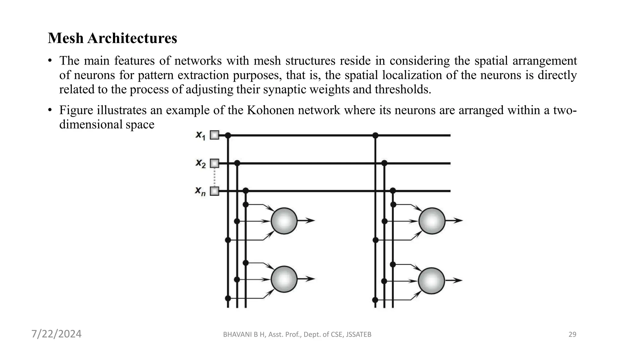
The document provides an overview of Artificial Neural Networks (ANNs), detailing their structure, functioning, and applications. It covers fundamental concepts such as perceptrons, multilayer networks, backpropagation algorithms, and the appropriate problems for ANN learning. Additionally, it explores various ANN architectures, including single-layer and multi-layer feedforward networks, as well as recurrent and mesh networks.
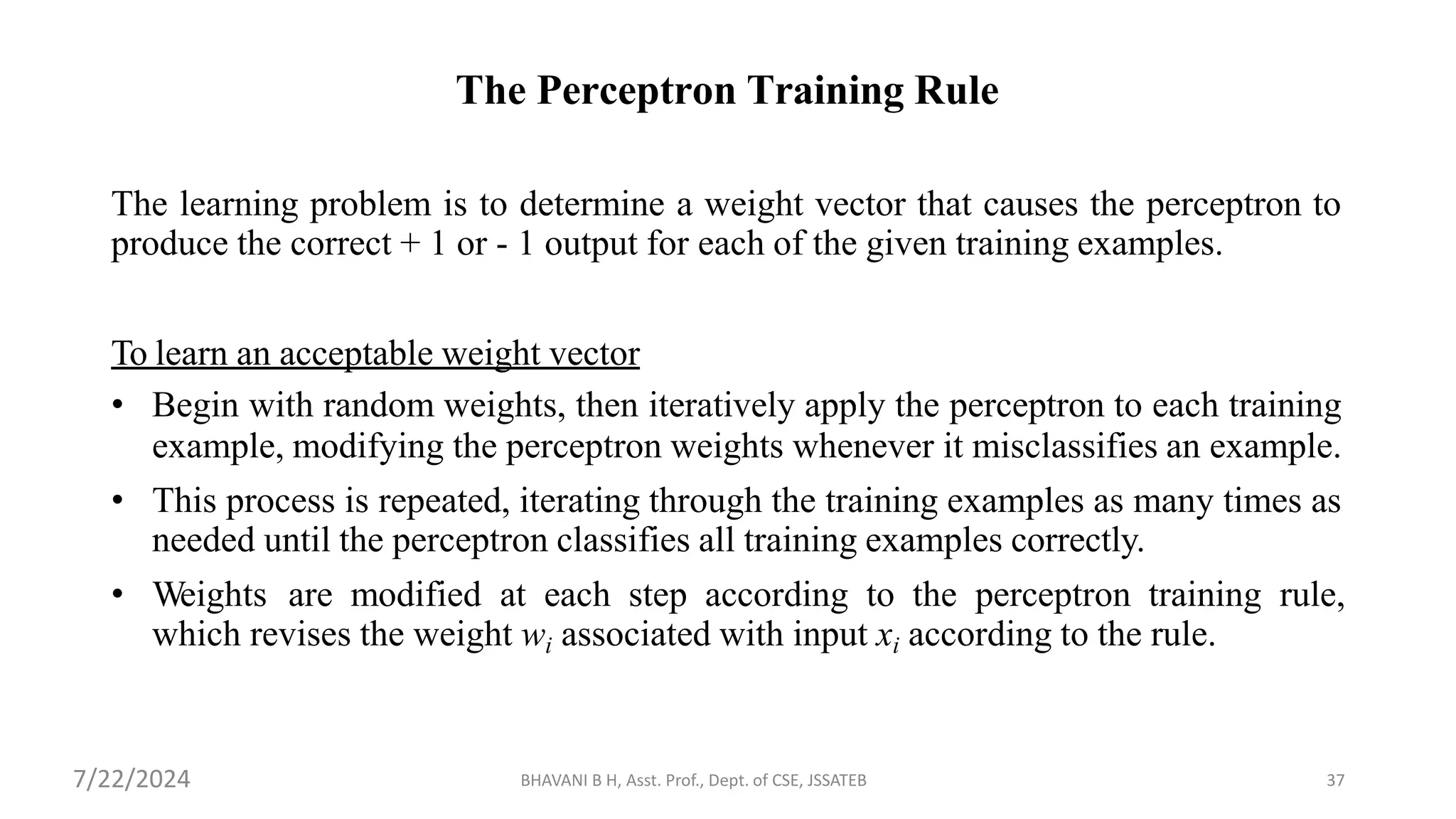
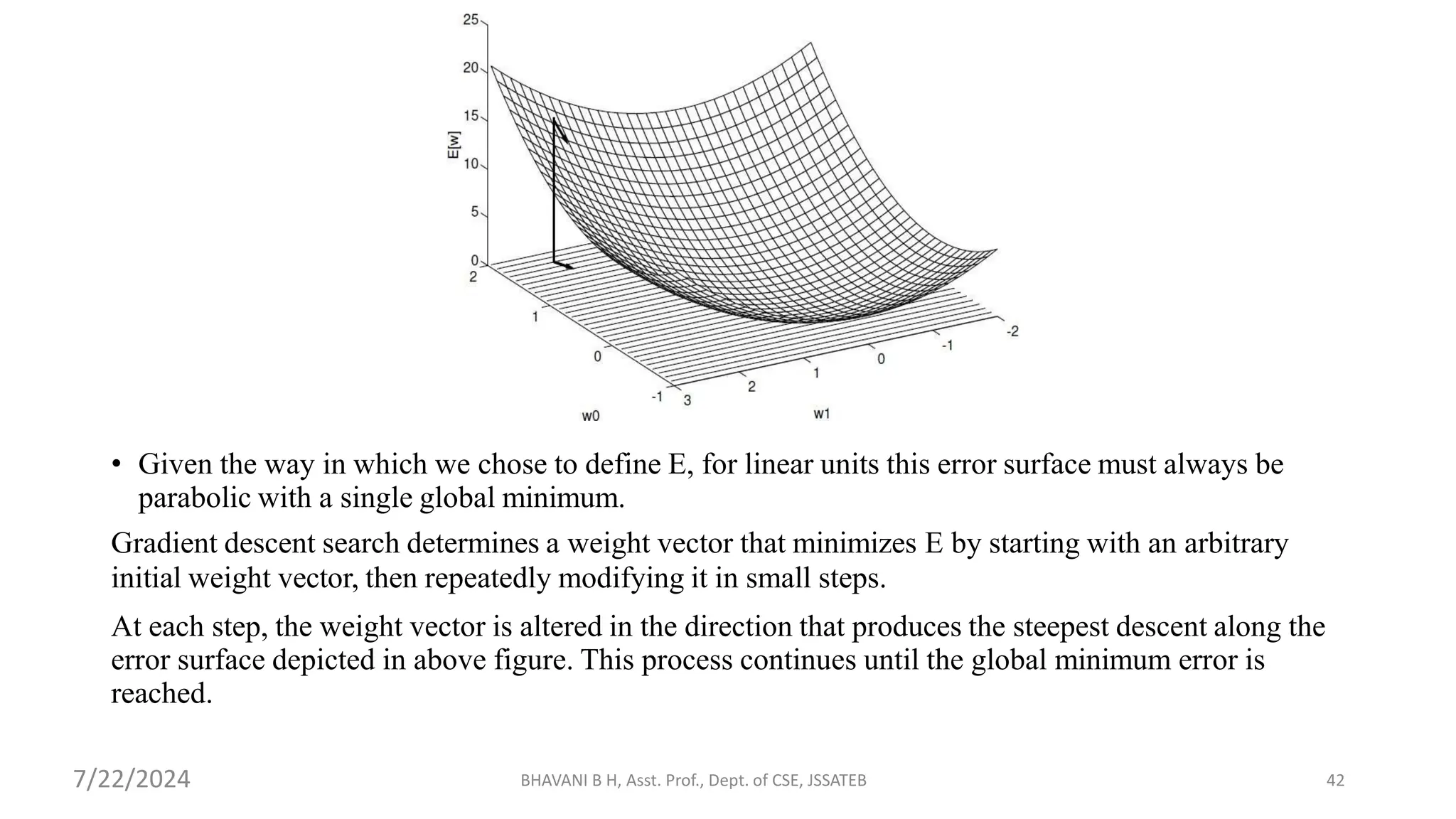
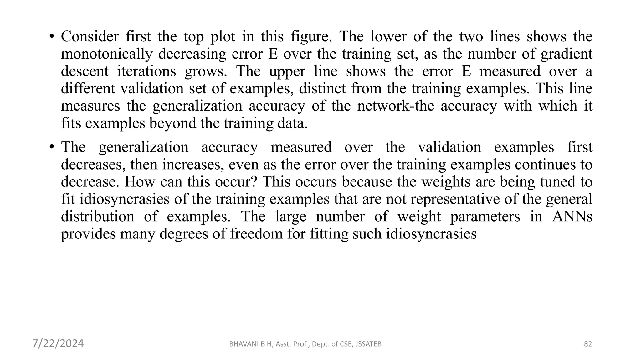
![To derive a weight learning rule for linear units, specify a measure for the training
error of a hypothesis (weight vector), relative to the training examples.
Where,
• D is the set of training examples,
• td is the target output for training example d,
• od is the output of the linear unit for training example d
• E [ w ] is simply half the squared difference between the target output td and the linear unit output
od, summed over all training examples.
BHAVANI B H, Asst. Prof., Dept. of CSE, JSSATEB 40
7/22/2024](https://image.slidesharecdn.com/artificialneuralnetworkmodule3ppt-240722160012-5eb00d91/75/Artificial-Neural-Network_module_3_ppt-pptx-40-2048.jpg)


![[DSC Europe 25] Andjelka Kovacevic - AI for the Deep Universe.pptx](https://cdn.slidesharecdn.com/ss_thumbnails/xdw54gniqhaq5svygbww-1-andjelka-kovacevic-ai-for-deep-universe-251203092157-8a1082b1-thumbnail.jpg?width=640&height=640&fit=bounds)


![[DSC Europe 25] Dragan Vucic - Building the Learning Organization - How AI Tr...](https://cdn.slidesharecdn.com/ss_thumbnails/8brigo2sbu6qur6gxrra-7-251205085715-6ae07d24-thumbnail.jpg?width=640&height=640&fit=bounds)
![[DSC Europe 25] Andy Cotgreave - Nothing is new in analytics.pptx](https://cdn.slidesharecdn.com/ss_thumbnails/mba4vzcurvoh5lfrd5zw-6-251205194645-341bbbbe-thumbnail.jpg?width=640&height=640&fit=bounds)
![[DSC Europe 25] Boris Perkovic - Lost in performance.pptx](https://cdn.slidesharecdn.com/ss_thumbnails/uq5hrp7vsuahqkxzifux-1-251204082258-fd2ee09d-thumbnail.jpg?width=640&height=640&fit=bounds)


![[DSC Europe 25] Marija Vlajkovic & Andrea Radonjanin - Integration of AI tool...](https://cdn.slidesharecdn.com/ss_thumbnails/qf1jrglttoc3bm8s3aop-final-integration-of-ai-tools-251208151905-394f3a6a-thumbnail.jpg?width=640&height=640&fit=bounds)


![[DSC Europe 25] Bogdan Daniel Maruneac - AI - It starts with you.pptx](https://cdn.slidesharecdn.com/ss_thumbnails/odov3snhrcqs9hx5ny2n-4-251205085715-f1daacfe-thumbnail.jpg?width=640&height=640&fit=bounds)