Announcements
§ Homework 8due today (Nov 7) at 11:59pm PT
§ Project 4 extended! Now due this Friday (Nov 10) at 11:59pm PT
§ HW 4 part 2 and HW 5 part 2 regrades at due this Friday (Nov 10)
at 11:59pm PT
2.
CS 188: ArtificialIntelligence
Perceptrons, Logistic Regression and Optimization
[These slides were created by Dan Klein, Pieter Abbeel, Anca Dragan, Sergey Levine. All CS188 materials are at http://ai.berkeley.edu.]
3.
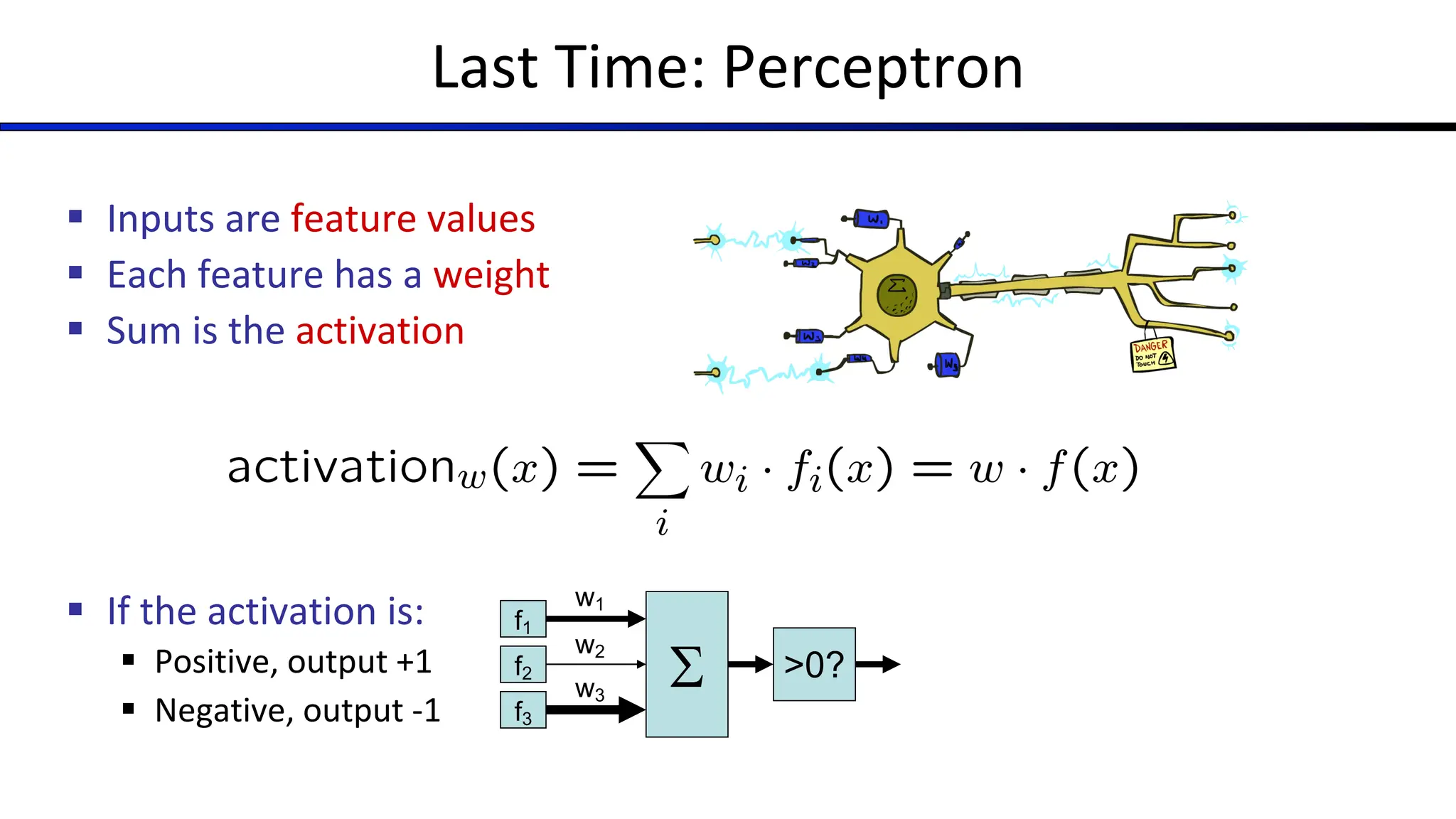
Last Time: Perceptron
§Inputs are feature values
§ Each feature has a weight
§ Sum is the activation
§ If the activation is:
§ Positive, output +1
§ Negative, output -1
S
f1
f2
f3
w1
w2
w3
>0?
4.
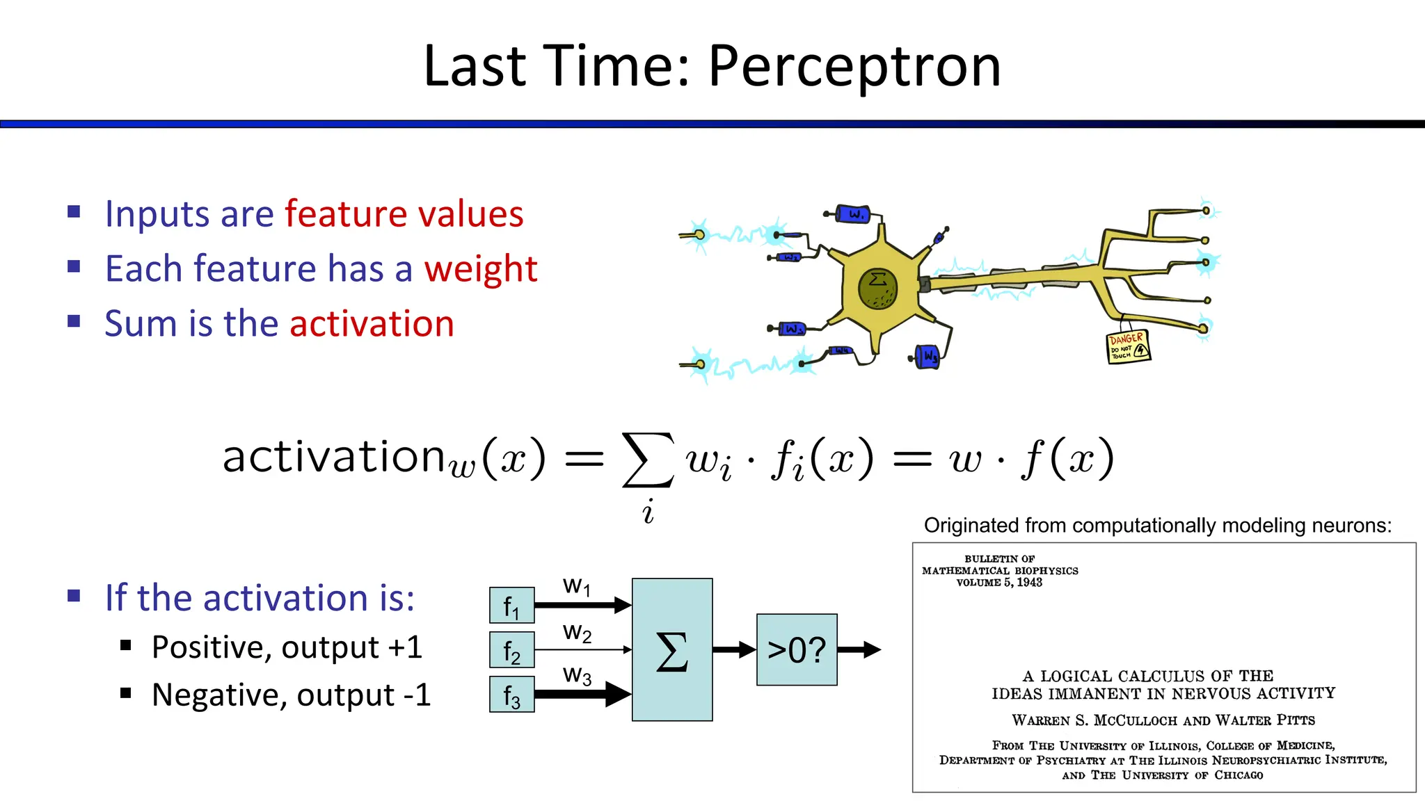
Last Time: Perceptron
§Inputs are feature values
§ Each feature has a weight
§ Sum is the activation
§ If the activation is:
§ Positive, output +1
§ Negative, output -1
S
f1
f2
f3
w1
w2
w3
>0?
Originated from computationally modeling neurons:
5.
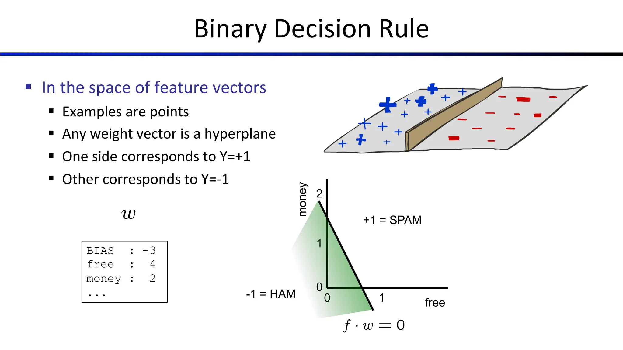
Binary Decision Rule
§In the space of feature vectors
§ Examples are points
§ Any weight vector is a hyperplane
§ One side corresponds to Y=+1
§ Other corresponds to Y=-1
BIAS : -3
free : 4
money : 2
...
0 1
0
1
2
free
money
+1 = SPAM
-1 = HAM
6.
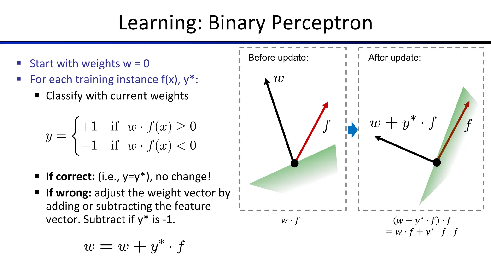
Learning: Binary Perceptron
§Start with weights w = 0
§ For each training instance f(x), y*:
§ Classify with current weights
§ If correct: (i.e., y=y*), no change!
§ If wrong: adjust the weight vector by
adding or subtracting the feature
vector. Subtract if y* is -1.
Before update: After update:
𝑤 ⋅ 𝑓 𝑤 + 𝑦∗
⋅ 𝑓 ⋅ 𝑓
= 𝑤 ⋅ 𝑓 + 𝑦∗ ⋅ 𝑓 ⋅ 𝑓
7.
???
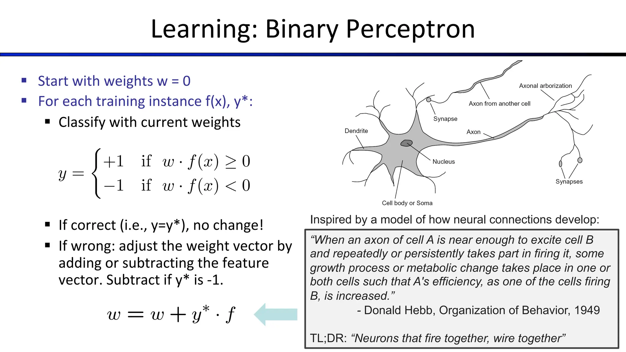
Learning: Binary Perceptron
§Start with weights w = 0
§ For each training instance f(x), y*:
§ Classify with current weights
§ If correct (i.e., y=y*), no change!
§ If wrong: adjust the weight vector by
adding or subtracting the feature
vector. Subtract if y* is -1.
“When an axon of cell A is near enough to excite cell B
and repeatedly or persistently takes part in firing it, some
growth process or metabolic change takes place in one or
both cells such that A's efficiency, as one of the cells firing
B, is increased.”
- Donald Hebb, Organization of Behavior, 1949
TL;DR: “Neurons that fire together, wire together”
Inspired by a model of how neural connections develop:
8.
Learning: Binary Perceptron
§Start with weights w = 0
§ For each training instance f(x), y*:
§ Classify with current weights
§ If correct (i.e., y=y*), no change!
§ If wrong: adjust the weight vector by
adding or subtracting the feature
vector. Subtract if y* is -1.
Hardware implementation built by Rosenblatt in 1957:
[Wikipedia]
9.
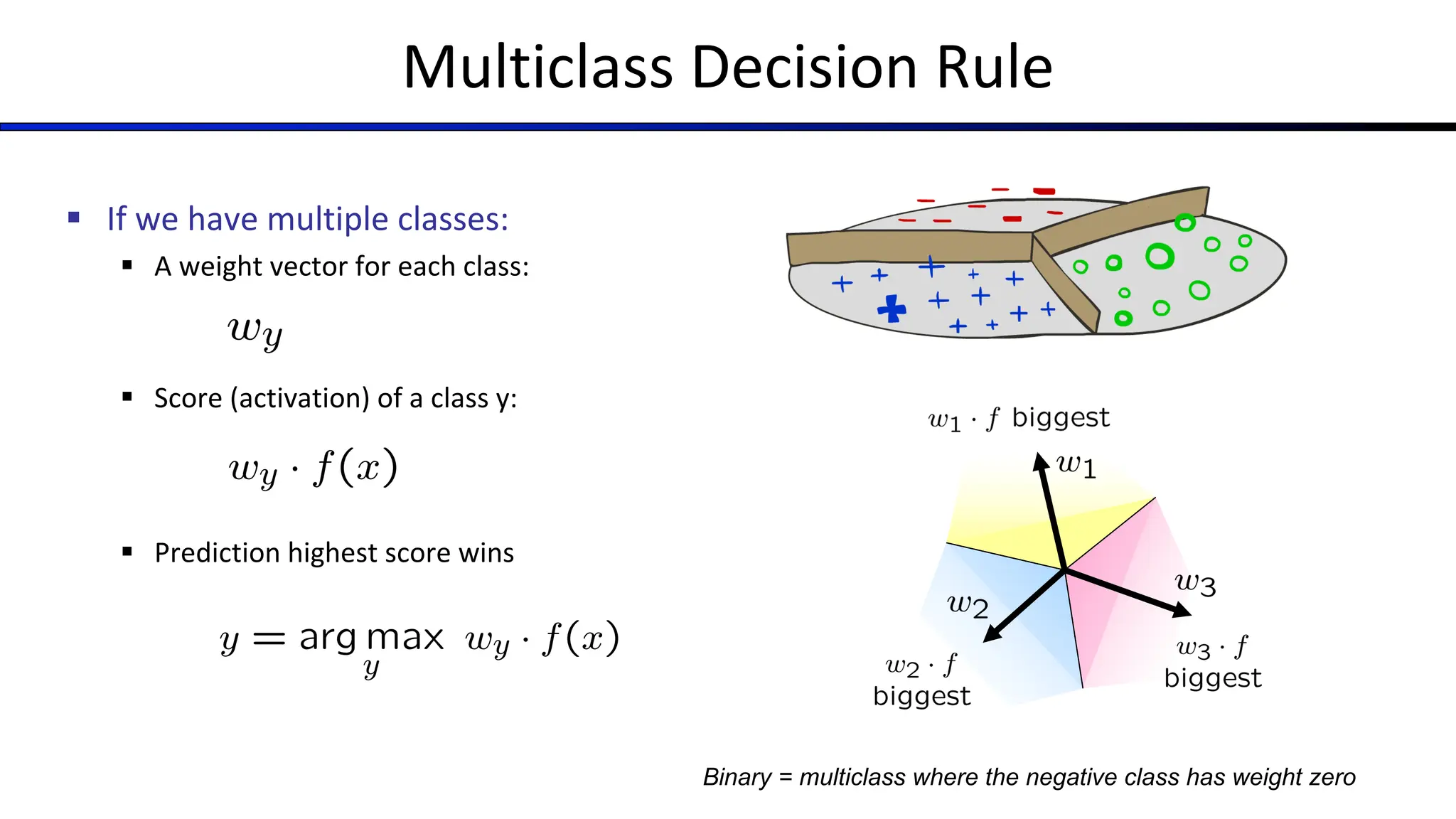
Multiclass Decision Rule
§If we have multiple classes:
§ A weight vector for each class:
§ Score (activation) of a class y:
§ Prediction highest score wins
Binary = multiclass where the negative class has weight zero
10.
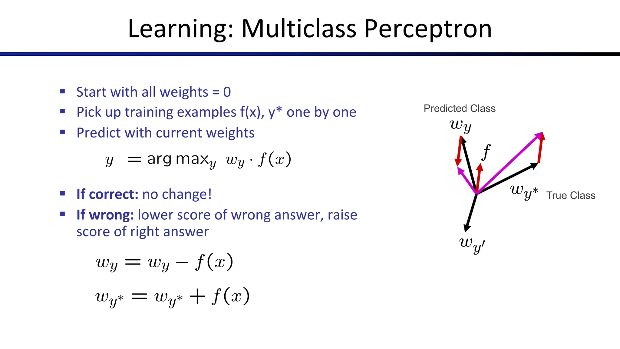
Learning: Multiclass Perceptron
§Start with all weights = 0
§ Pick up training examples f(x), y* one by one
§ Predict with current weights
§ If correct: no change!
§ If wrong: lower score of wrong answer, raise
score of right answer
Predicted Class
True Class
11.
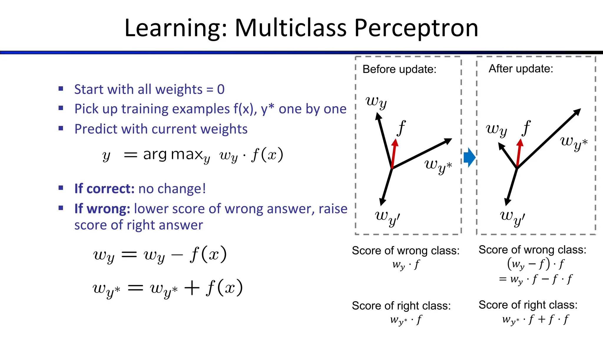
Learning: Multiclass Perceptron
§Start with all weights = 0
§ Pick up training examples f(x), y* one by one
§ Predict with current weights
§ If correct: no change!
§ If wrong: lower score of wrong answer, raise
score of right answer
Before update: After update:
Score of wrong class:
𝑤" ⋅ 𝑓
Score of right class:
𝑤"∗ ⋅ 𝑓
Score of wrong class:
𝑤" − 𝑓 ⋅ 𝑓
= 𝑤" ⋅ 𝑓 − 𝑓 ⋅ 𝑓
Score of right class:
𝑤"∗ ⋅ 𝑓 + 𝑓 ⋅ 𝑓
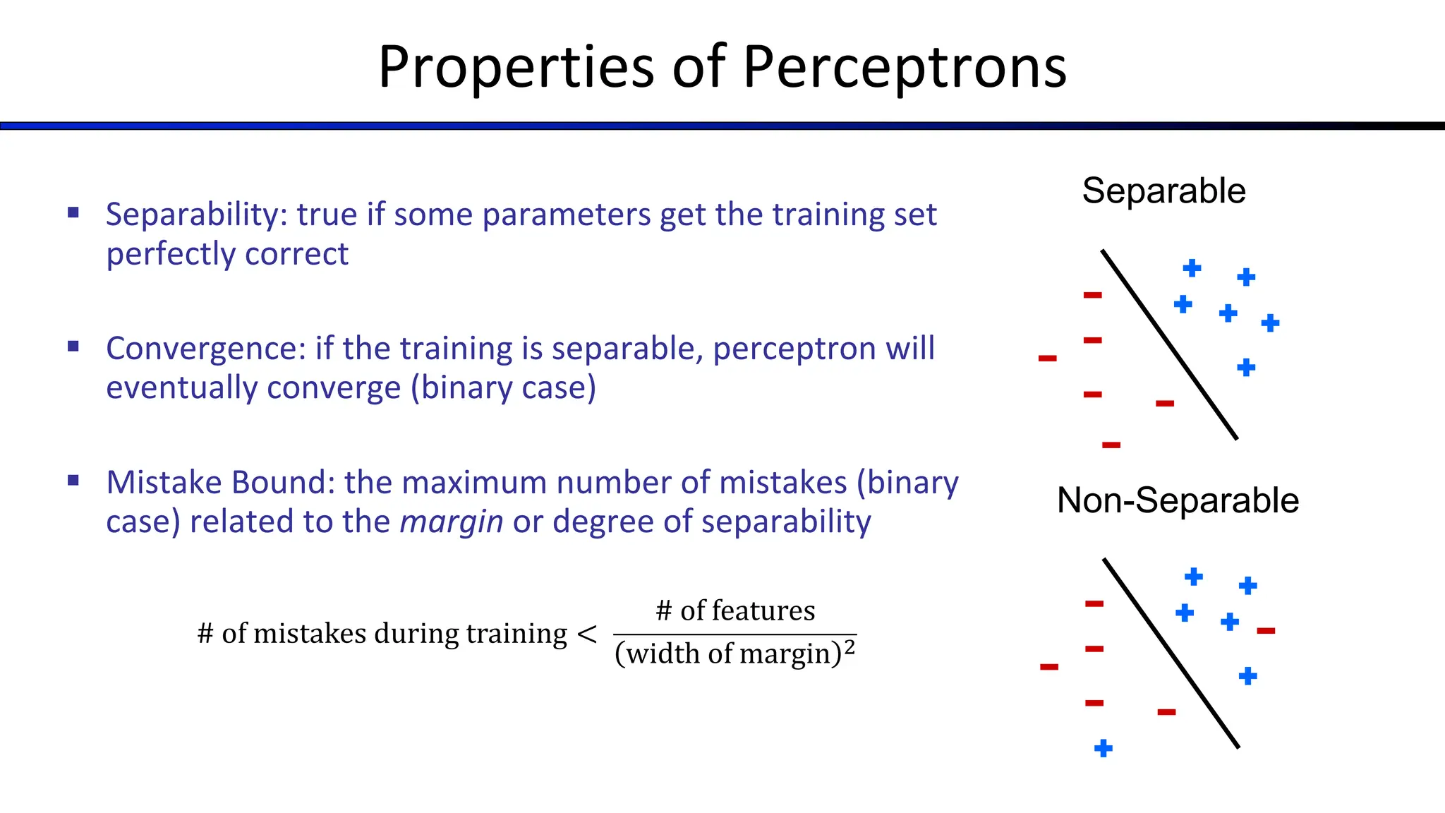
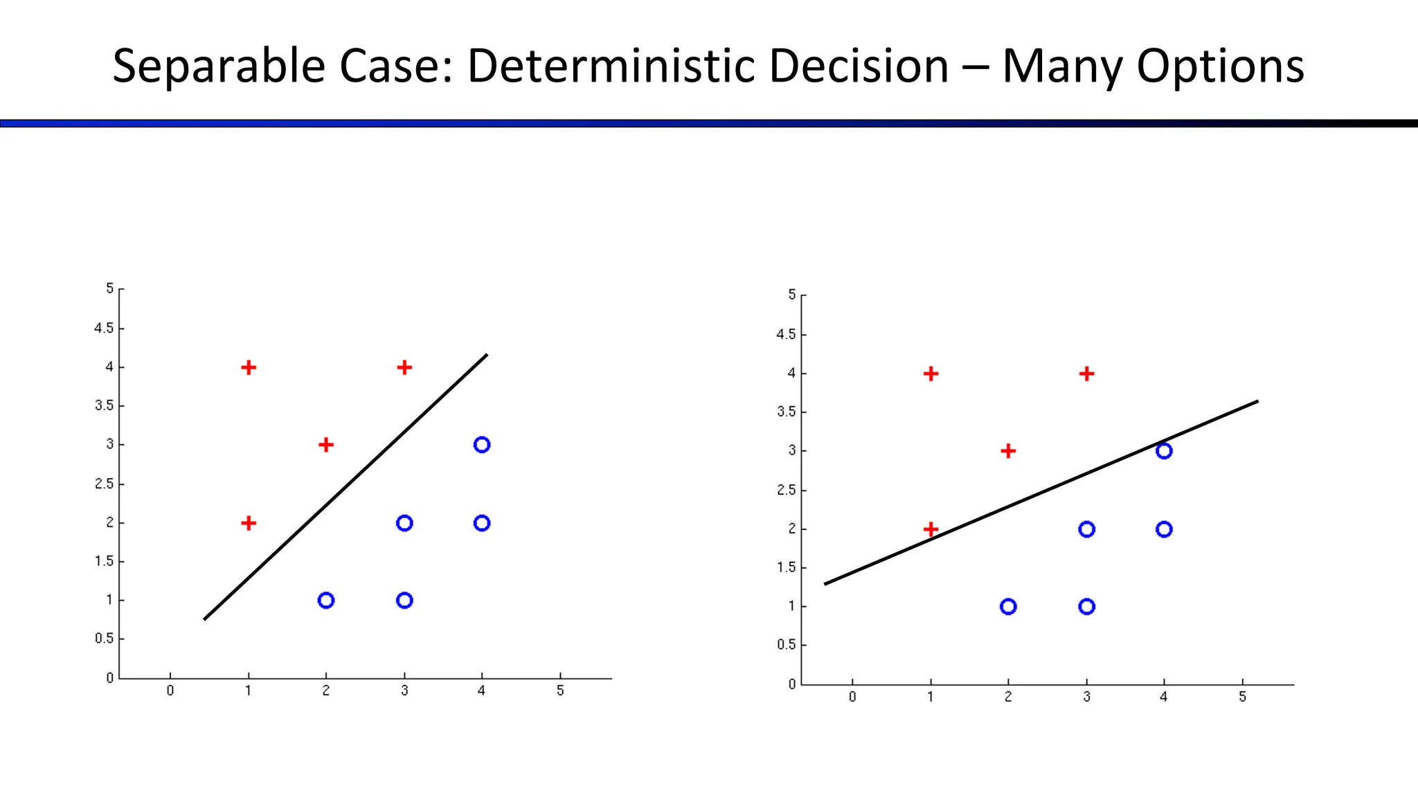
Properties of Perceptrons
§Separability: true if some parameters get the training set
perfectly correct
§ Convergence: if the training is separable, perceptron will
eventually converge (binary case)
§ Mistake Bound: the maximum number of mistakes (binary
case) related to the margin or degree of separability
Separable
Non-Separable
# of mistakes during training <
# of features
width of margin !
14.
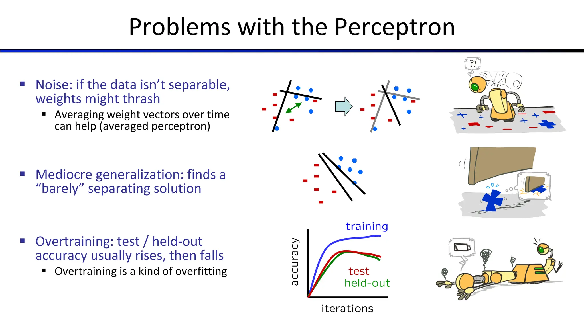
Problems with thePerceptron
§ Noise: if the data isn’t separable,
weights might thrash
§ Averaging weight vectors over time
can help (averaged perceptron)
§ Mediocre generalization: finds a
“barely” separating solution
§ Overtraining: test / held-out
accuracy usually rises, then falls
§ Overtraining is a kind of overfitting
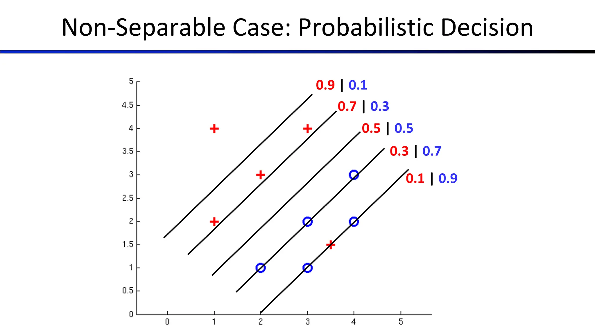
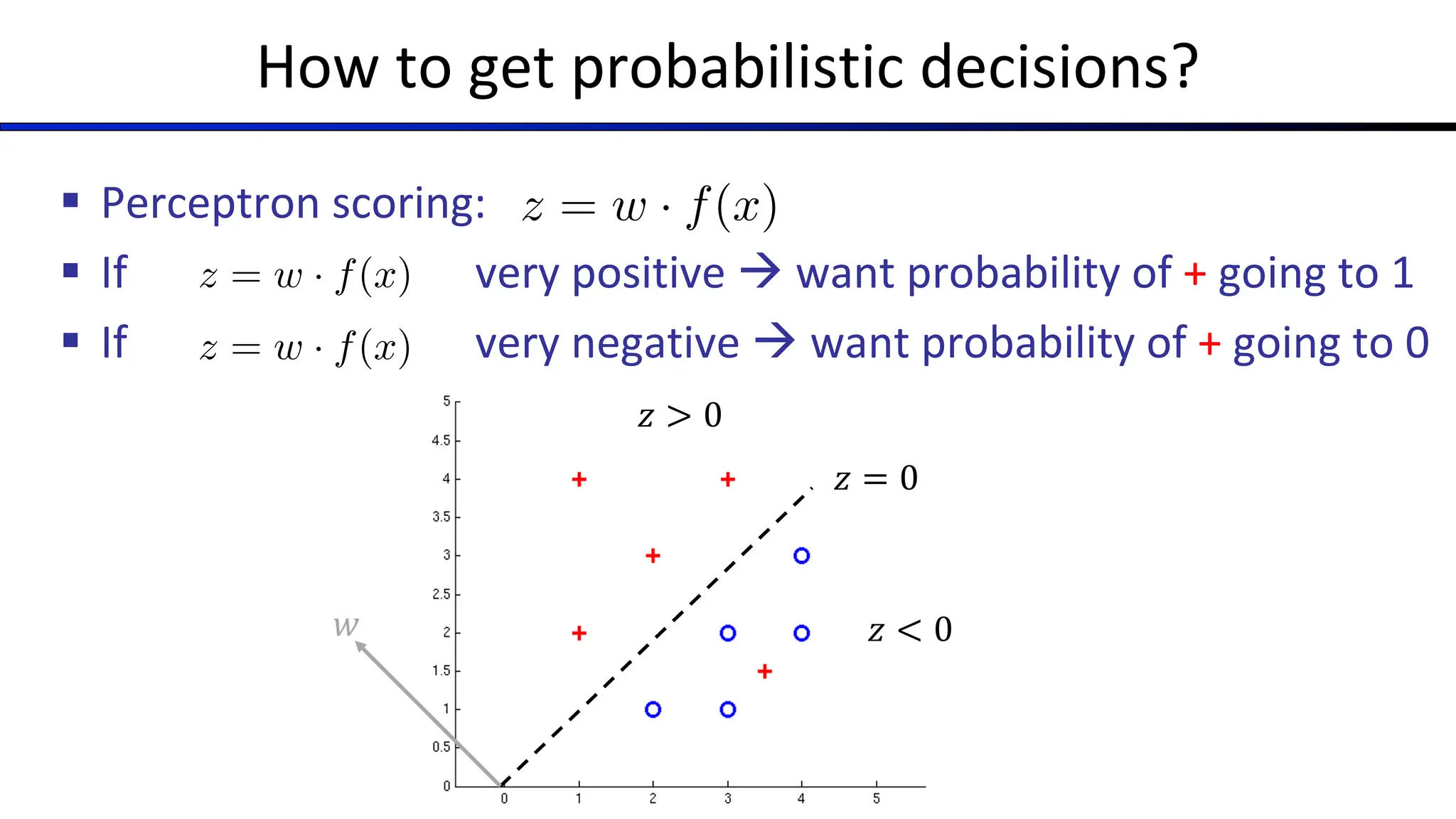
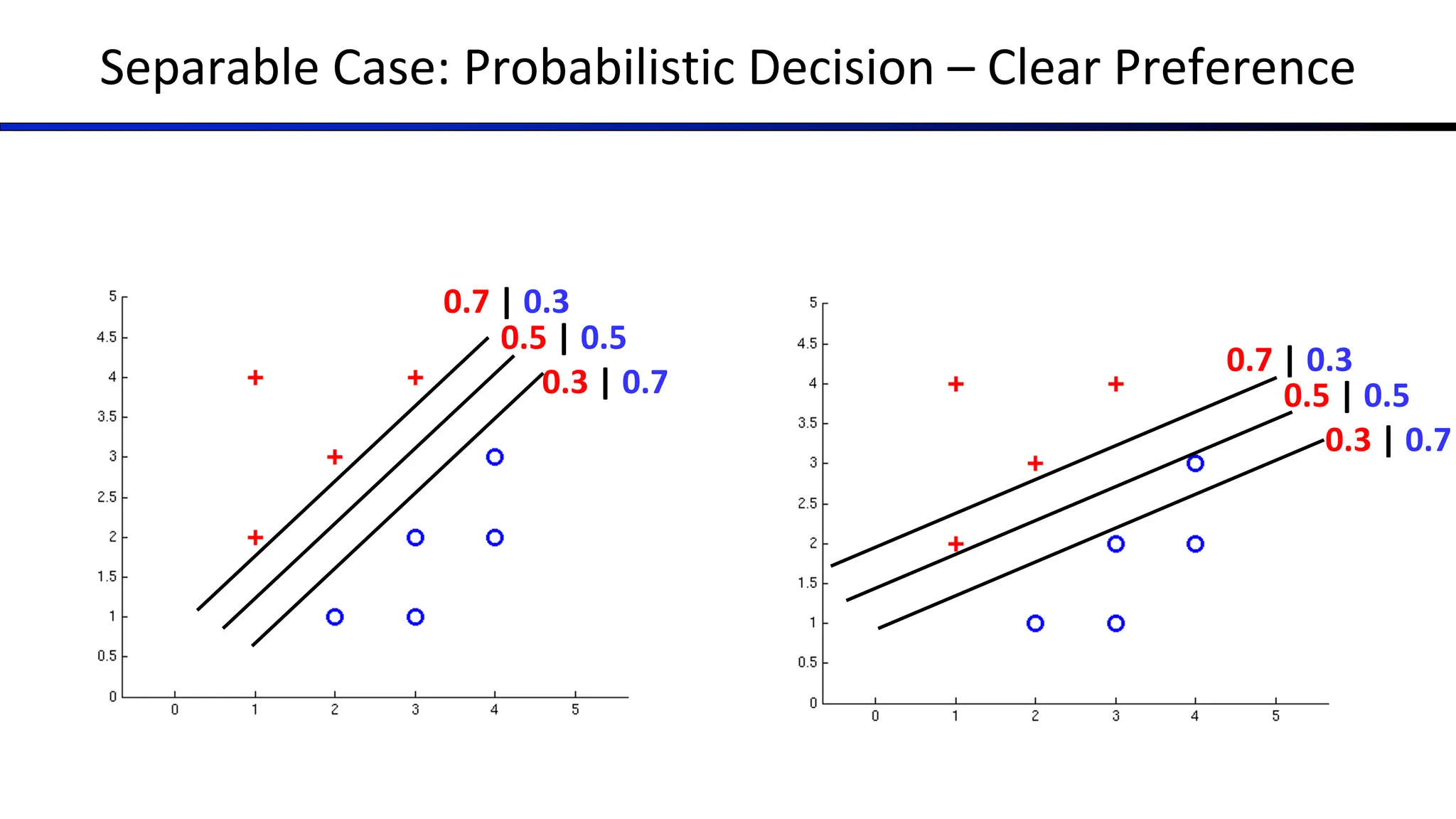
How to getprobabilistic decisions?
§ Perceptron scoring:
§ If very positive à want probability of + going to 1
§ If very negative à want probability of + going to 0
z = w · f(x)
z = w · f(x)
z = w · f(x)
𝑧 = 0
𝑤
𝑧 > 0
𝑧 < 0
19.
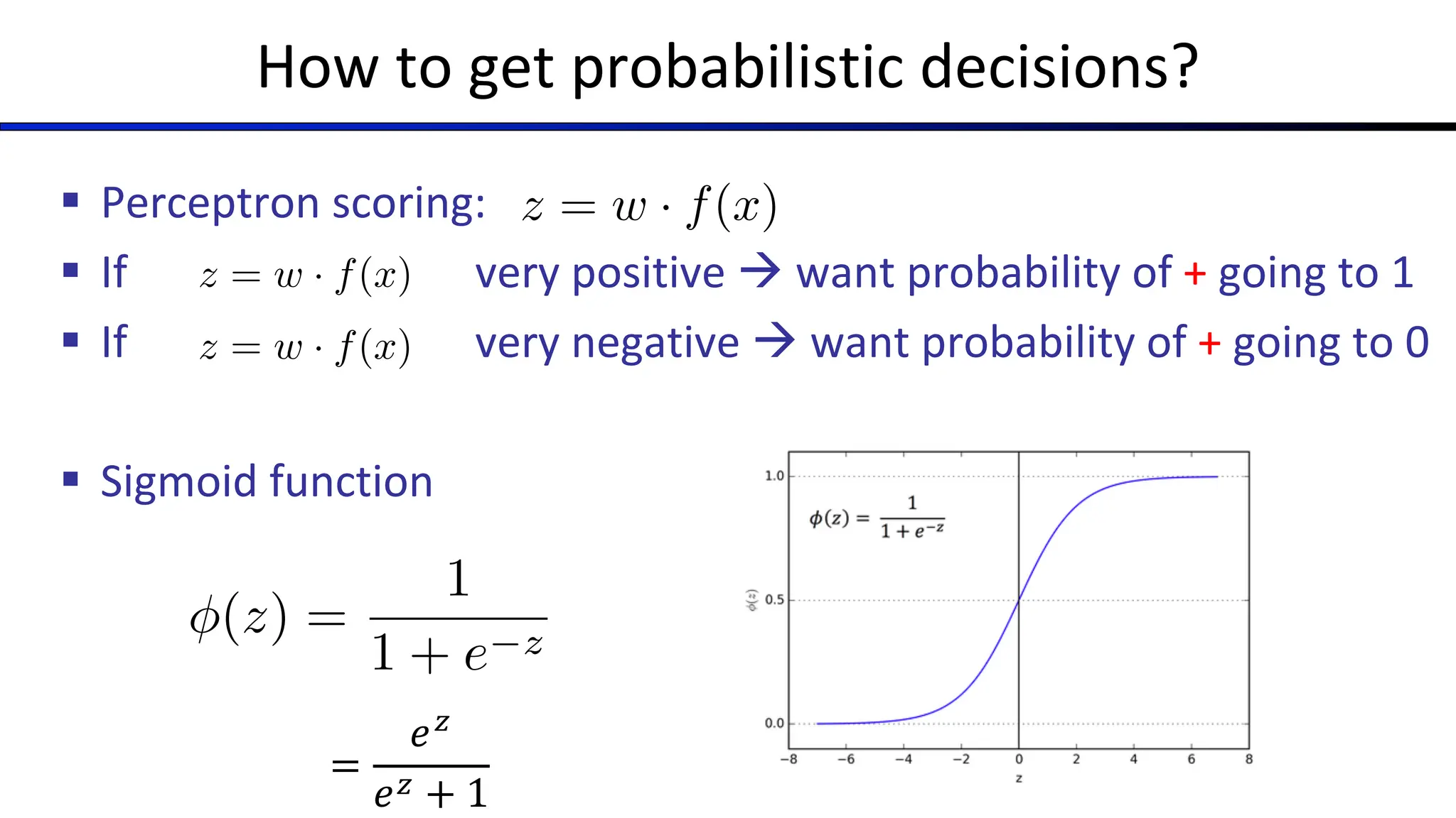
How to getprobabilistic decisions?
§ Perceptron scoring:
§ If very positive à want probability of + going to 1
§ If very negative à want probability of + going to 0
§ Sigmoid function
z = w · f(x)
z = w · f(x)
z = w · f(x)
(z) =
1
1 + e z
=
𝑒4
𝑒4 + 1
20.
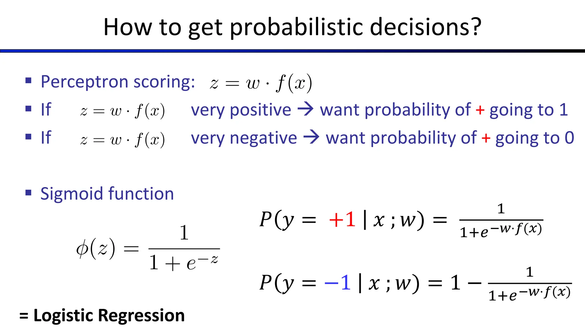
How to getprobabilistic decisions?
§ Perceptron scoring:
§ If very positive à want probability of + going to 1
§ If very negative à want probability of + going to 0
§ Sigmoid function
z = w · f(x)
z = w · f(x)
z = w · f(x)
(z) =
1
1 + e z
= Logistic Regression
𝑃 𝑦 = +1 𝑥 ; 𝑤) =
!
!"#!"⋅$(&)
𝑃 𝑦 = −1 𝑥 ; 𝑤) = 1 −
!
!"#!"⋅$(&)
21.
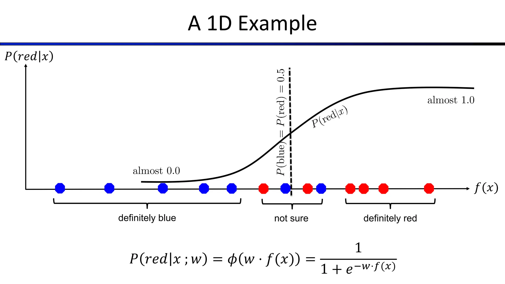
A 1D Example
definitelyblue definitely red
not sure
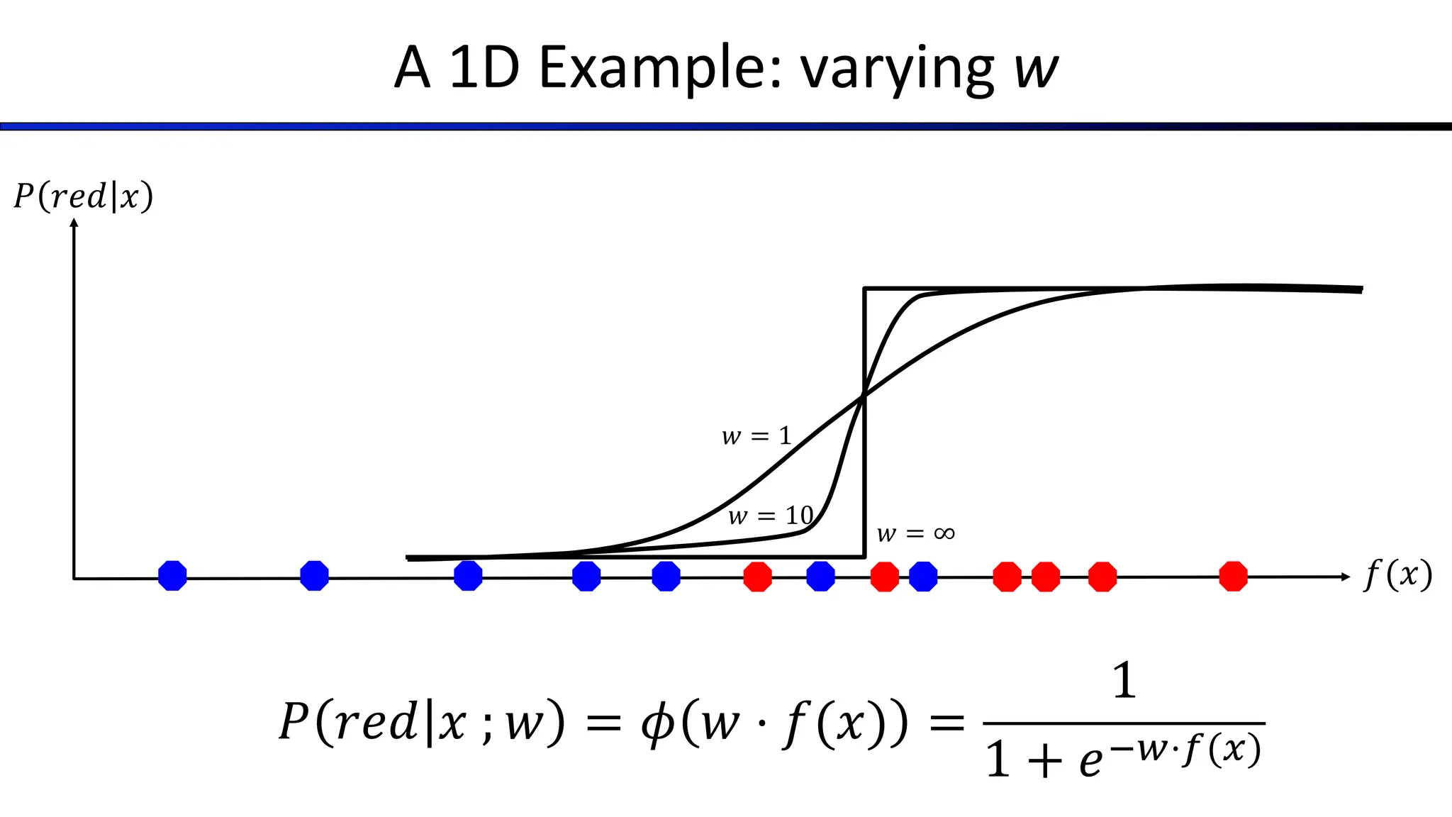
𝑃 𝑟𝑒𝑑 𝑥 ; 𝑤 = 𝜙 𝑤 ⋅ 𝑓(𝑥) =
1
1 + 𝑒56⋅8(:)
𝑃 𝑟𝑒𝑑 𝑥
𝑓(𝑥)
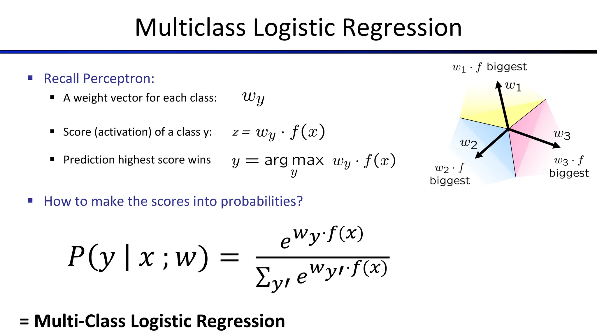
Multiclass Logistic Regression
§Recall Perceptron:
§ A weight vector for each class:
§ Score (activation) of a class y: z =
§ Prediction highest score wins
§ How to make the scores into probabilities?
§ In general: softmax 𝑧,, . . . , 𝑧- = [
.!"
∑ 0!#
, … ,
.!$
∑ 0!#
]
z1, z2, z3 !
ez1
ez1 + ez2 + ez3
,
ez2
ez1 + ez2 + ez3
,
ez3
ez1 + ez2 + ez3
original activations softmax activations
29.
Multiclass Logistic Regression
§Recall Perceptron:
§ A weight vector for each class:
§ Score (activation) of a class y: z =
§ Prediction highest score wins
§ How to make the scores into probabilities?
= Multi-Class Logistic Regression
𝑃 𝑦 𝑥 ; 𝑤) =
!!"⋅$(&)
∑"( !!"(⋅$(&)
30.
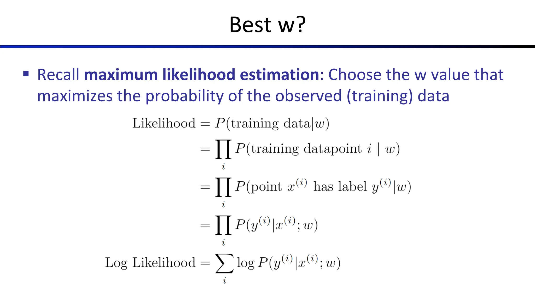
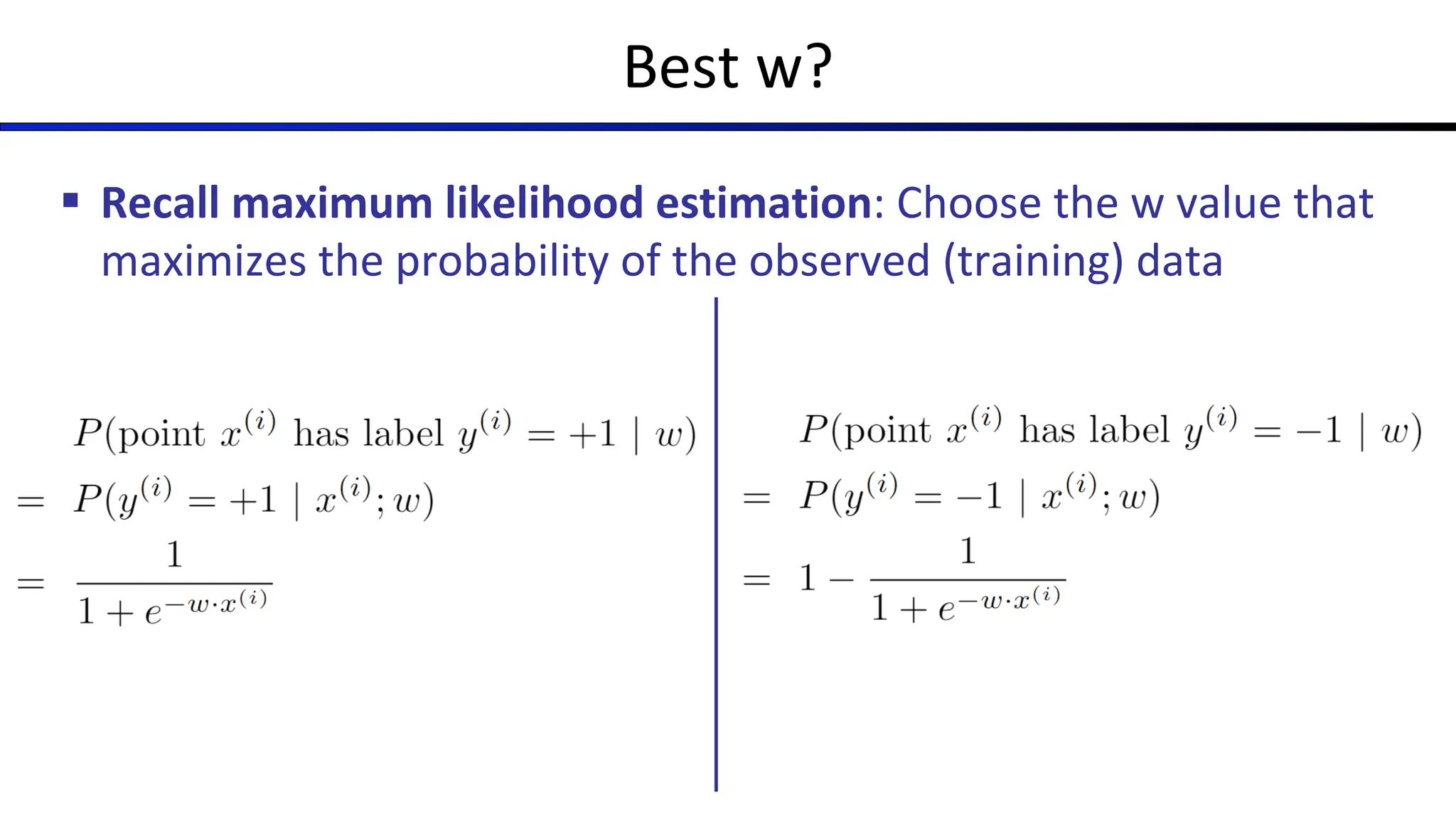
Best w?
§ Recallmaximum likelihood estimation: Choose the w value that
maximizes the probability of the observed (training) data
31.
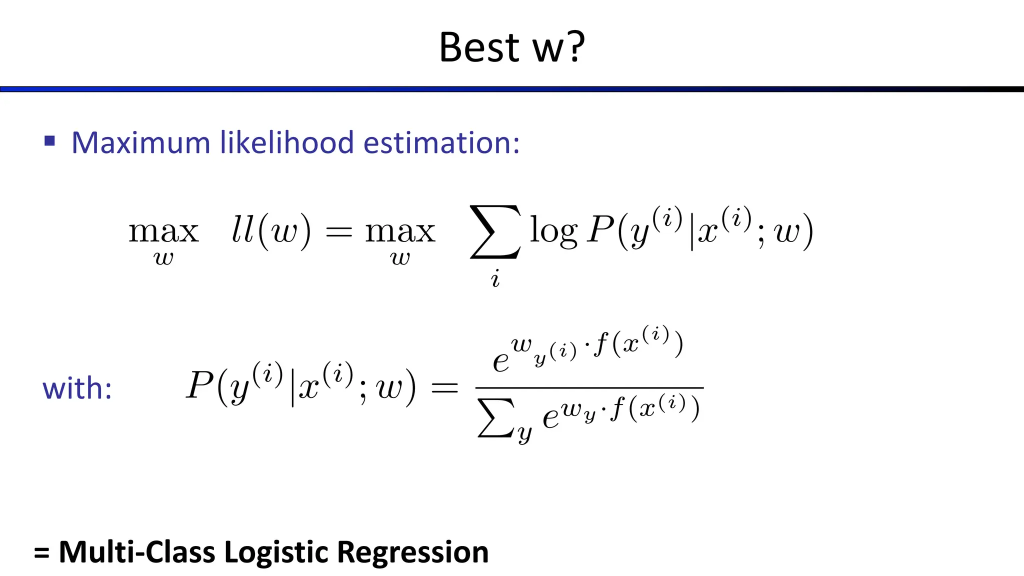
Best w?
§ Maximumlikelihood estimation:
with:
max
w
ll(w) = max
w
X
i
log P(y(i)
|x(i)
; w)
P(y(i)
|x(i)
; w) =
e
wy(i) ·f(x(i)
)
P
y ewy·f(x(i))
= Multi-Class Logistic Regression
32.
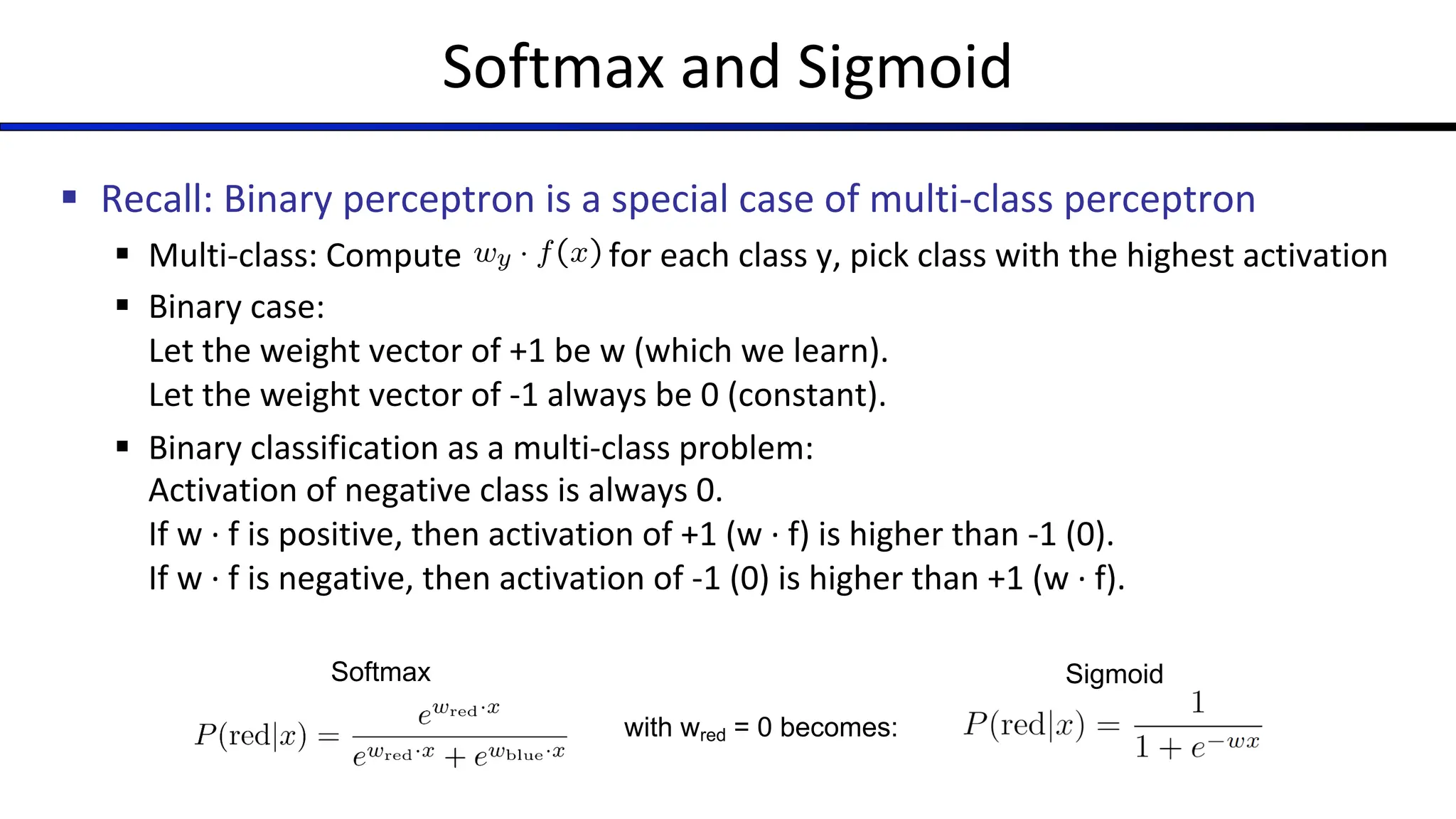
Softmax and Sigmoid
§Recall: Binary perceptron is a special case of multi-class perceptron
§ Multi-class: Compute for each class y, pick class with the highest activation
§ Binary case:
Let the weight vector of +1 be w (which we learn).
Let the weight vector of -1 always be 0 (constant).
§ Binary classification as a multi-class problem:
Activation of negative class is always 0.
If w · f is positive, then activation of +1 (w · f) is higher than -1 (0).
If w · f is negative, then activation of -1 (0) is higher than +1 (w · f).
Softmax
with wred = 0 becomes:
Sigmoid
33.
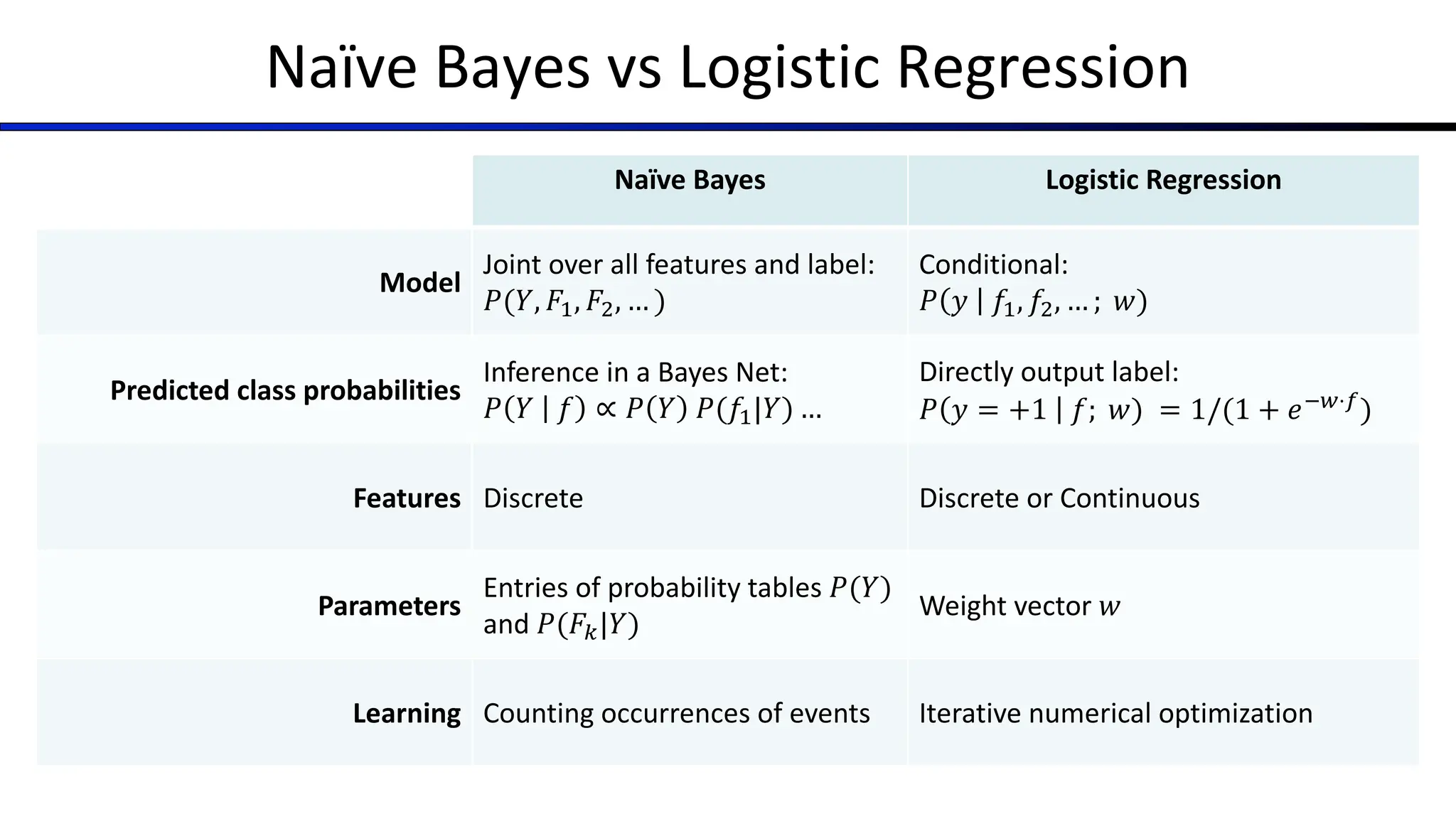
Naïve Bayes vsLogistic Regression
Naïve Bayes Logistic Regression
Model
Joint over all features and label:
𝑃(𝑌, 𝐹", 𝐹!, … )
Conditional:
𝑃 𝑦 𝑓", 𝑓!, … ; 𝑤)
Predicted class probabilities
Inference in a Bayes Net:
𝑃 𝑌 𝑓 ∝ 𝑃 𝑌 𝑃(𝑓"|𝑌) …
Directly output label:
𝑃 𝑦 = +1 𝑓; 𝑤) = 1/(1 + 𝑒#$⋅&)
Features Discrete Discrete or Continuous
Parameters
Entries of probability tables 𝑃(𝑌)
and 𝑃(𝐹'|𝑌)
Weight vector 𝑤
Learning Counting occurrences of events Iterative numerical optimization
34.
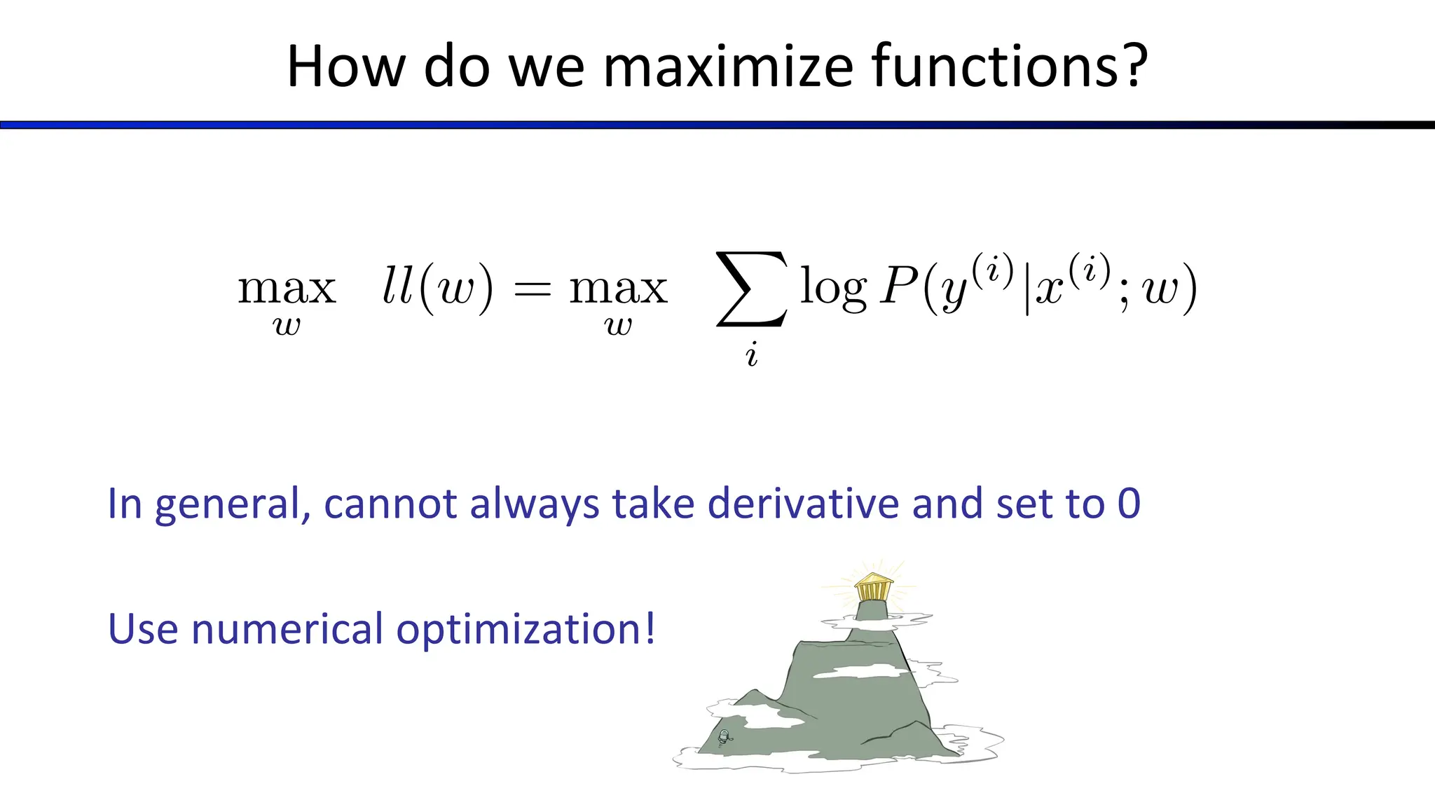
How do wemaximize functions?
In general, cannot always take derivative and set to 0
Use numerical optimization!
max
w
ll(w) = max
w
X
i
log P(y(i)
|x(i)
; w)
35.
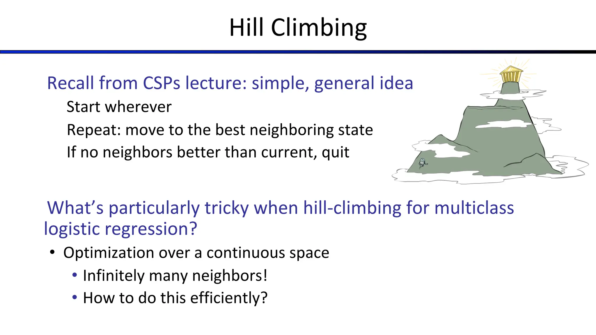
Hill Climbing
Recall fromCSPs lecture: simple, general idea
Start wherever
Repeat: move to the best neighboring state
If no neighbors better than current, quit
What’s particularly tricky when hill-climbing for multiclass
logistic regression?
• Optimization over a continuous space
• Infinitely many neighbors!
• How to do this efficiently?

![CS 188: Artificial Intelligence
Perceptrons, Logistic Regression and Optimization
[These slides were created by Dan Klein, Pieter Abbeel, Anca Dragan, Sergey Levine. All CS188 materials are at http://ai.berkeley.edu.]](https://image.slidesharecdn.com/cs188-fa23-lec221-250917101120-f6329e0a/75/Ai-notes-useful-for-btech-part-2-ai-notes-pdf-2-2048.jpg)
![Learning: Binary Perceptron
§ Start with weights w = 0
§ For each training instance f(x), y*:
§ Classify with current weights
§ If correct (i.e., y=y*), no change!
§ If wrong: adjust the weight vector by
adding or subtracting the feature
vector. Subtract if y* is -1.
Hardware implementation built by Rosenblatt in 1957:
[Wikipedia]](https://image.slidesharecdn.com/cs188-fa23-lec221-250917101120-f6329e0a/75/Ai-notes-useful-for-btech-part-2-ai-notes-pdf-8-2048.jpg)
![Example: Multiclass Perceptron
Iteration 0: x: “win the vote” f(x): [1 1 0 1 1] y*: politics
Iteration 1: x: “win the election” f(x): [1 1 0 0 1] y*: politics
Iteration 2: x: “win the game” f(x): [1 1 1 0 1] y*: sports
BIAS
win
game
vote
the
1
0
0
0
0
1
𝑤 ⋅ 𝑓 𝑥 :
0
-1
0
-1
-1
-2
0
-1
0
-1
-1
-2
1
0
1
-1
0
BIAS
win
game
vote
the
0
0
0
0
0
0
𝑤 ⋅ 𝑓 𝑥 :
1
1
0
1
1
3
1
1
0
1
1
3
0
0
-1
1
0
BIAS
win
game
vote
the
0
0
0
0
0
0
𝑤 ⋅ 𝑓 𝑥 :
0
0
0
0
0
0
0
0
0
0
0
0
0
0
0
0
0](https://image.slidesharecdn.com/cs188-fa23-lec221-250917101120-f6329e0a/75/Ai-notes-useful-for-btech-part-2-ai-notes-pdf-12-2048.jpg)

![Multiclass Logistic Regression
§ Recall Perceptron:
§ A weight vector for each class:
§ Score (activation) of a class y: z =
§ Prediction highest score wins
§ How to make the scores into probabilities?
§ In general: softmax 𝑧,, . . . , 𝑧- = [
.!"
∑ 0!#
, … ,
.!$
∑ 0!#
]
z1, z2, z3 !
ez1
ez1 + ez2 + ez3
,
ez2
ez1 + ez2 + ez3
,
ez3
ez1 + ez2 + ez3
original activations softmax activations](https://image.slidesharecdn.com/cs188-fa23-lec221-250917101120-f6329e0a/75/Ai-notes-useful-for-btech-part-2-ai-notes-pdf-28-2048.jpg)