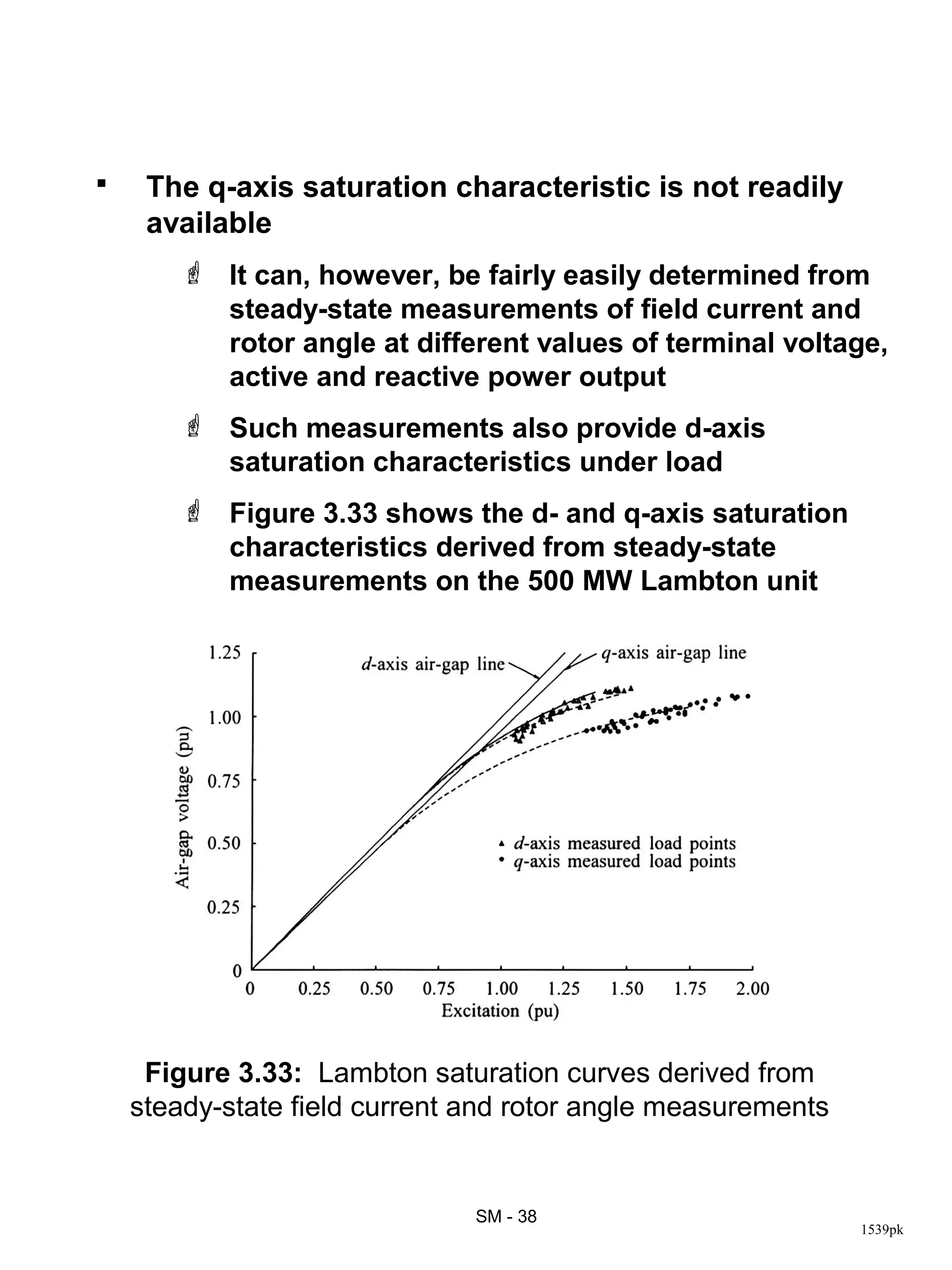
The document provides an overview of synchronous machines, including:
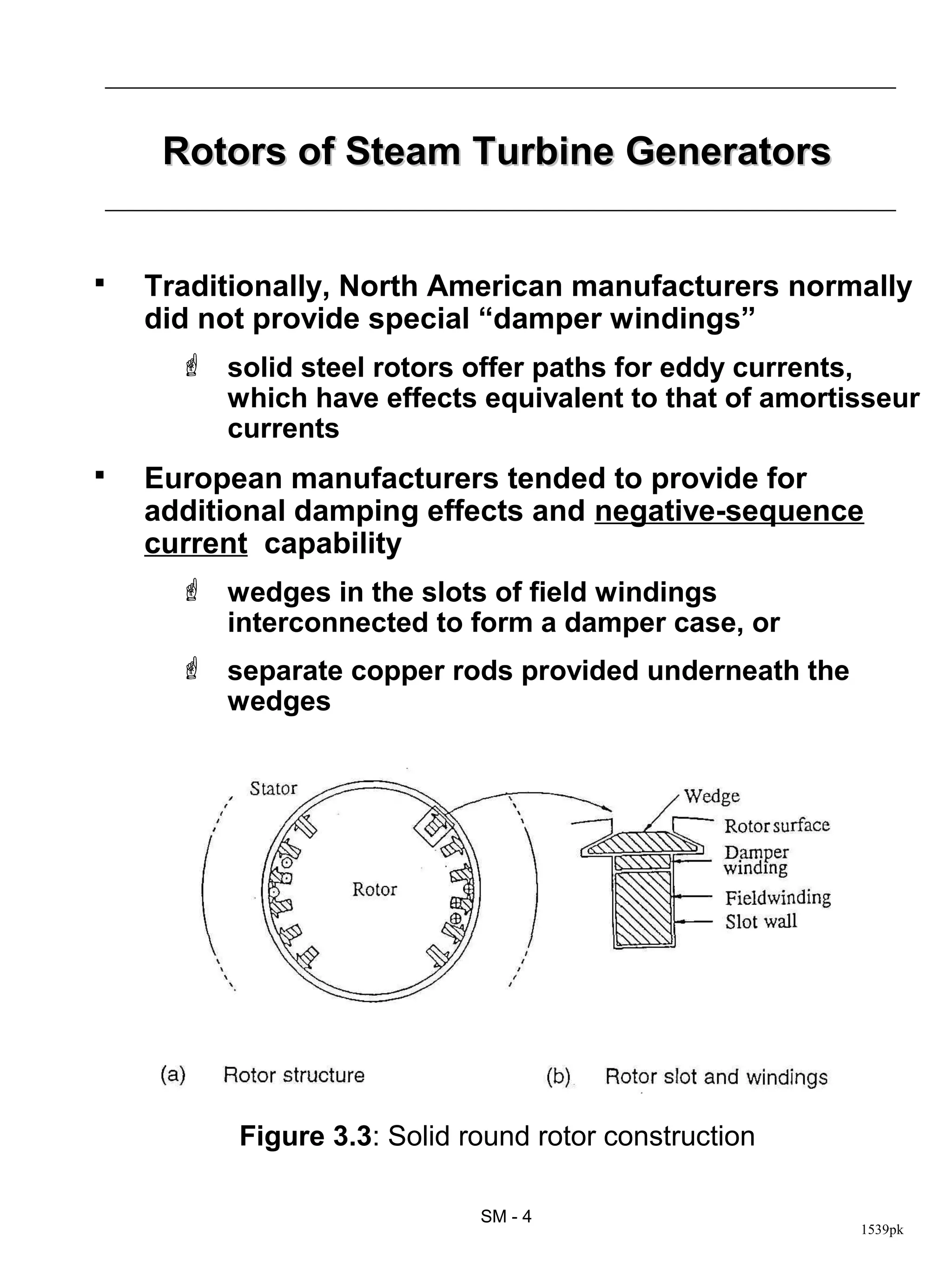
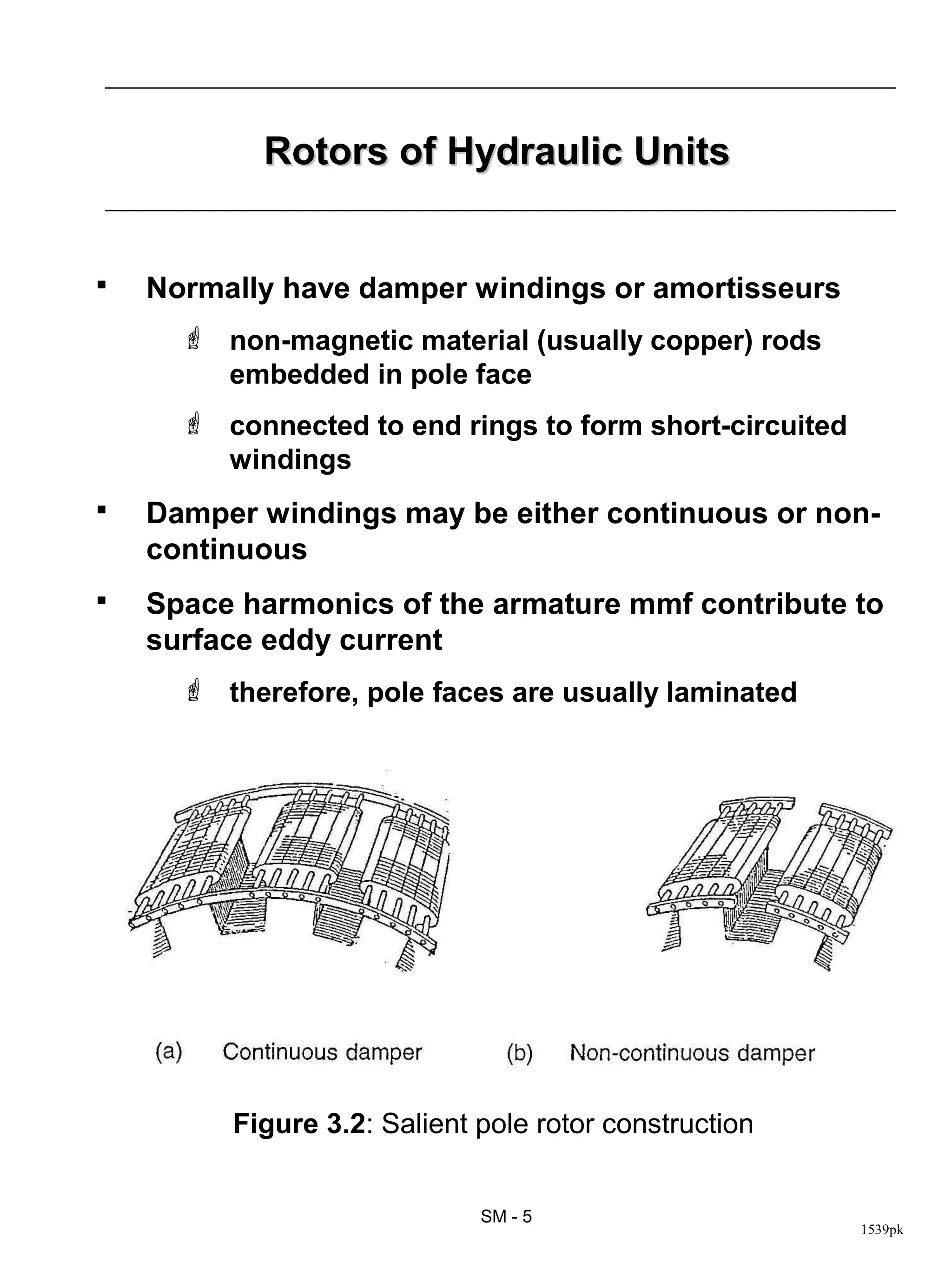
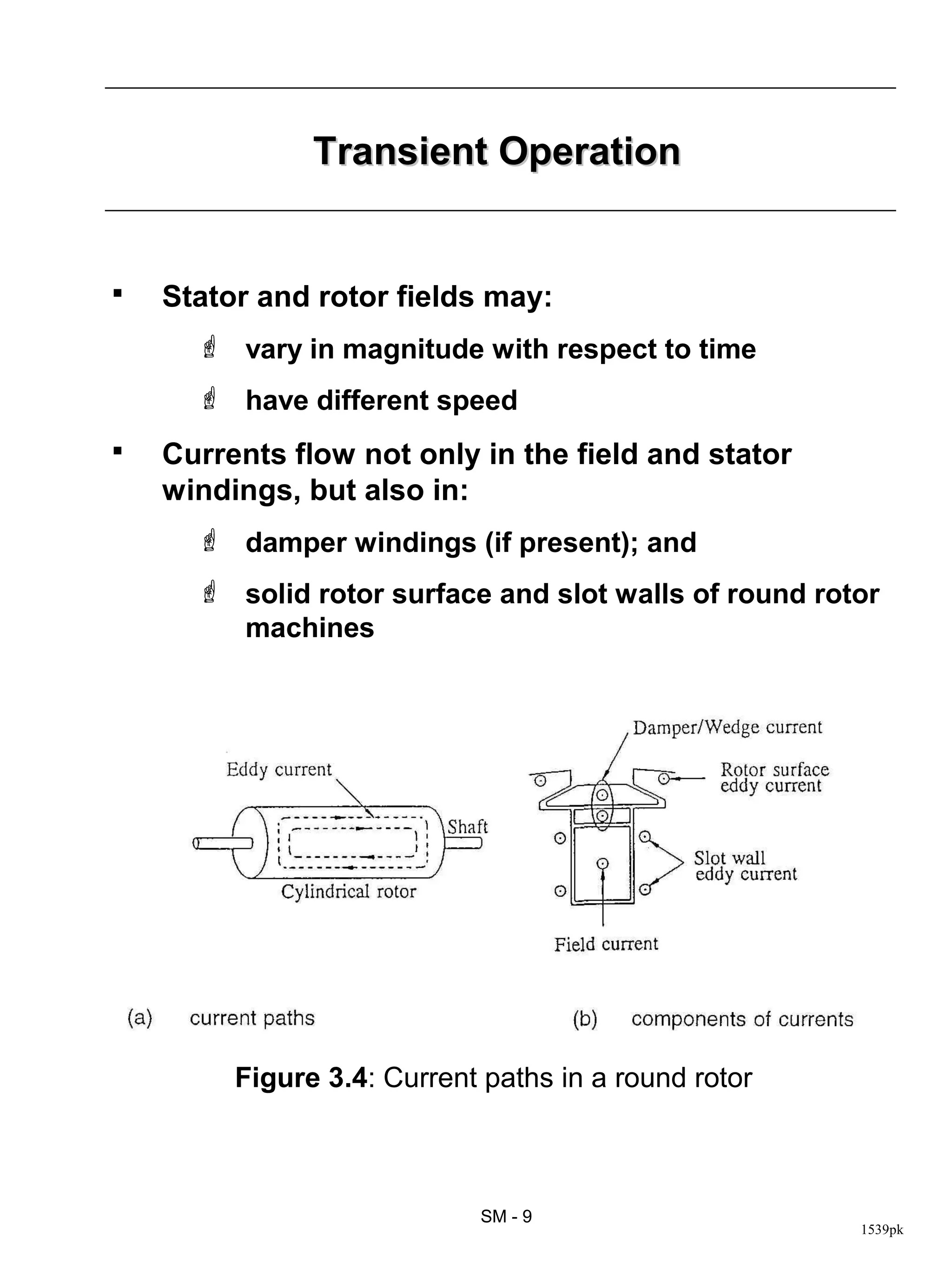
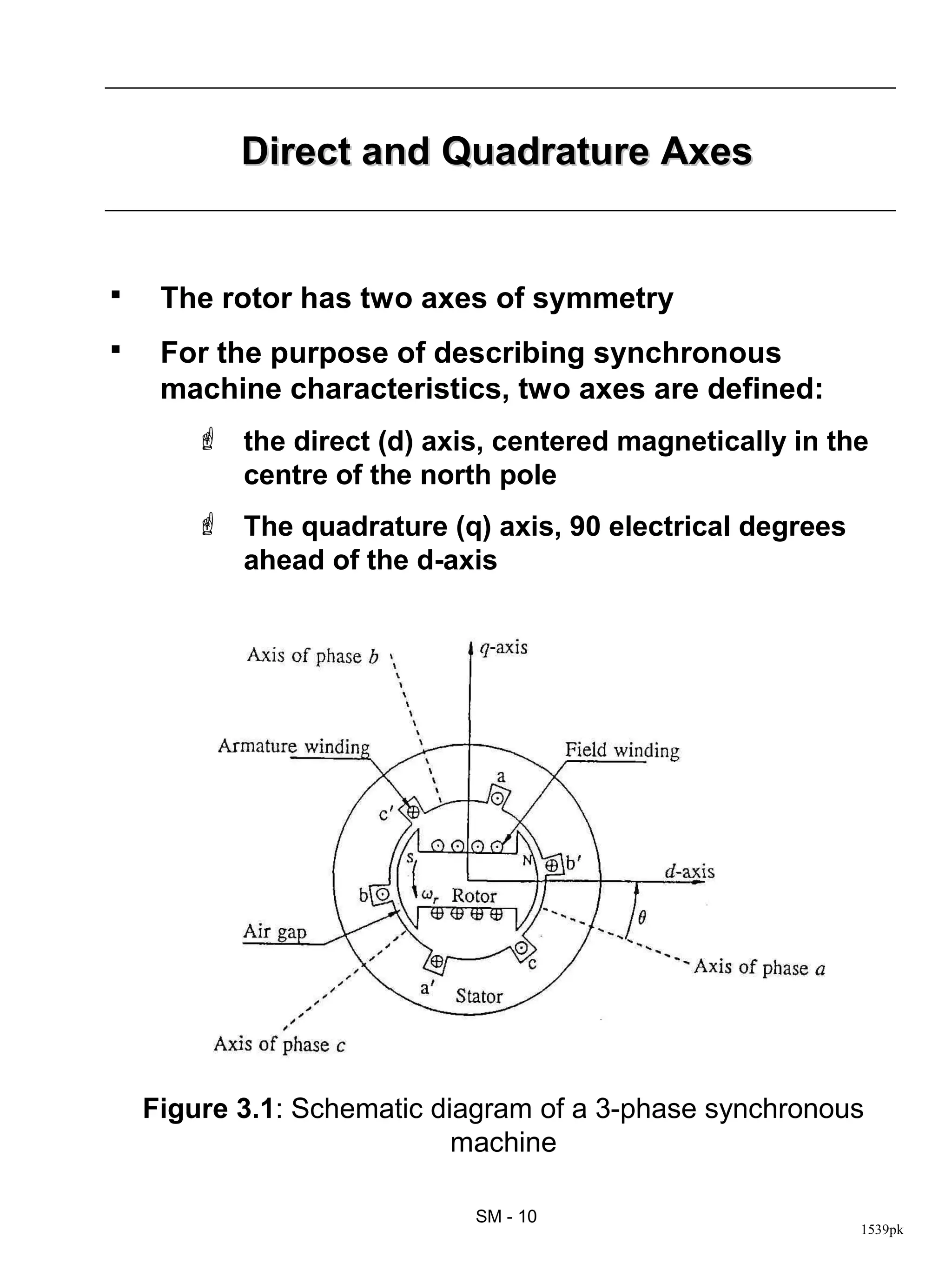
1. Their physical description with salient pole and round rotor structures.
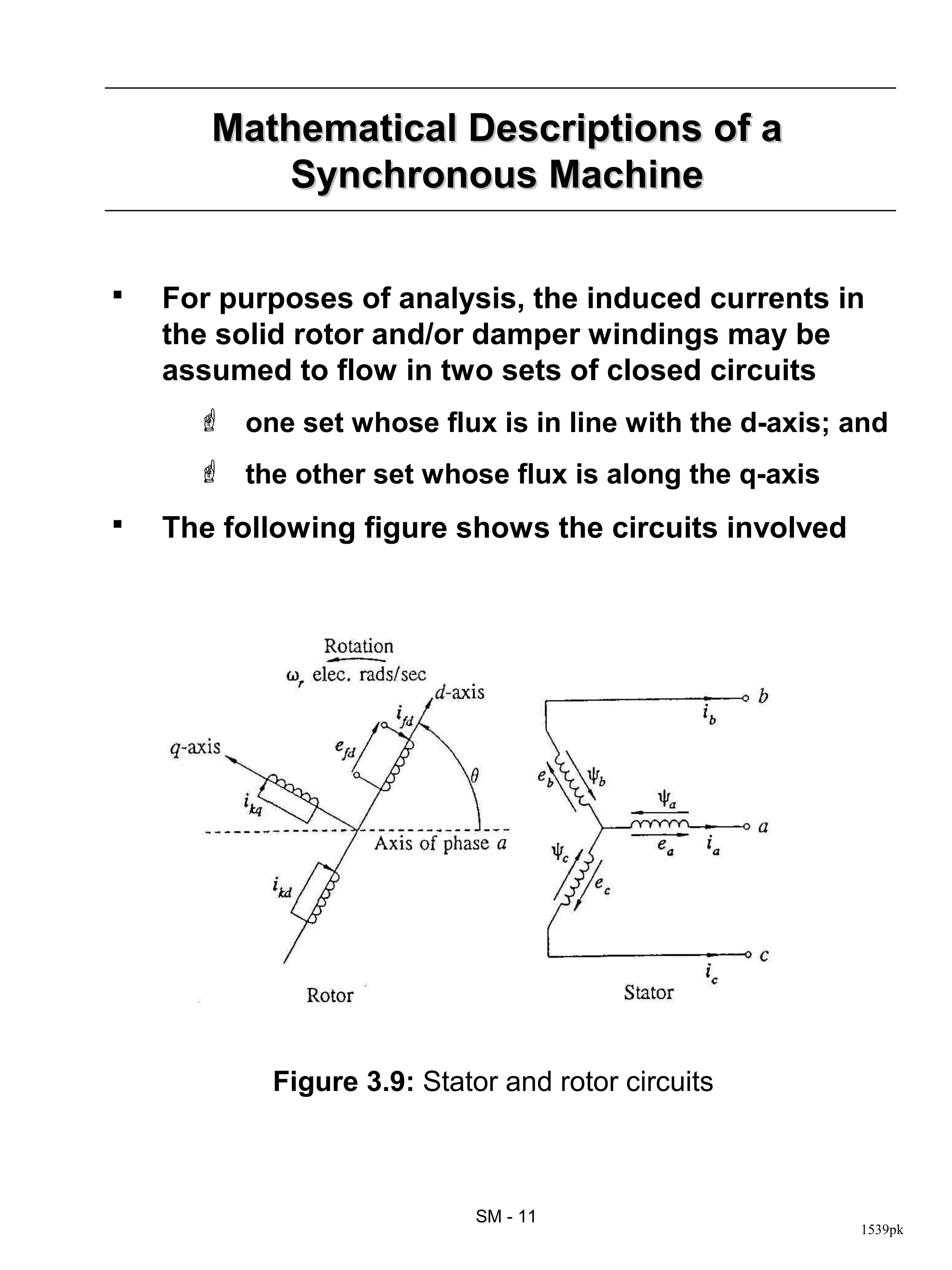
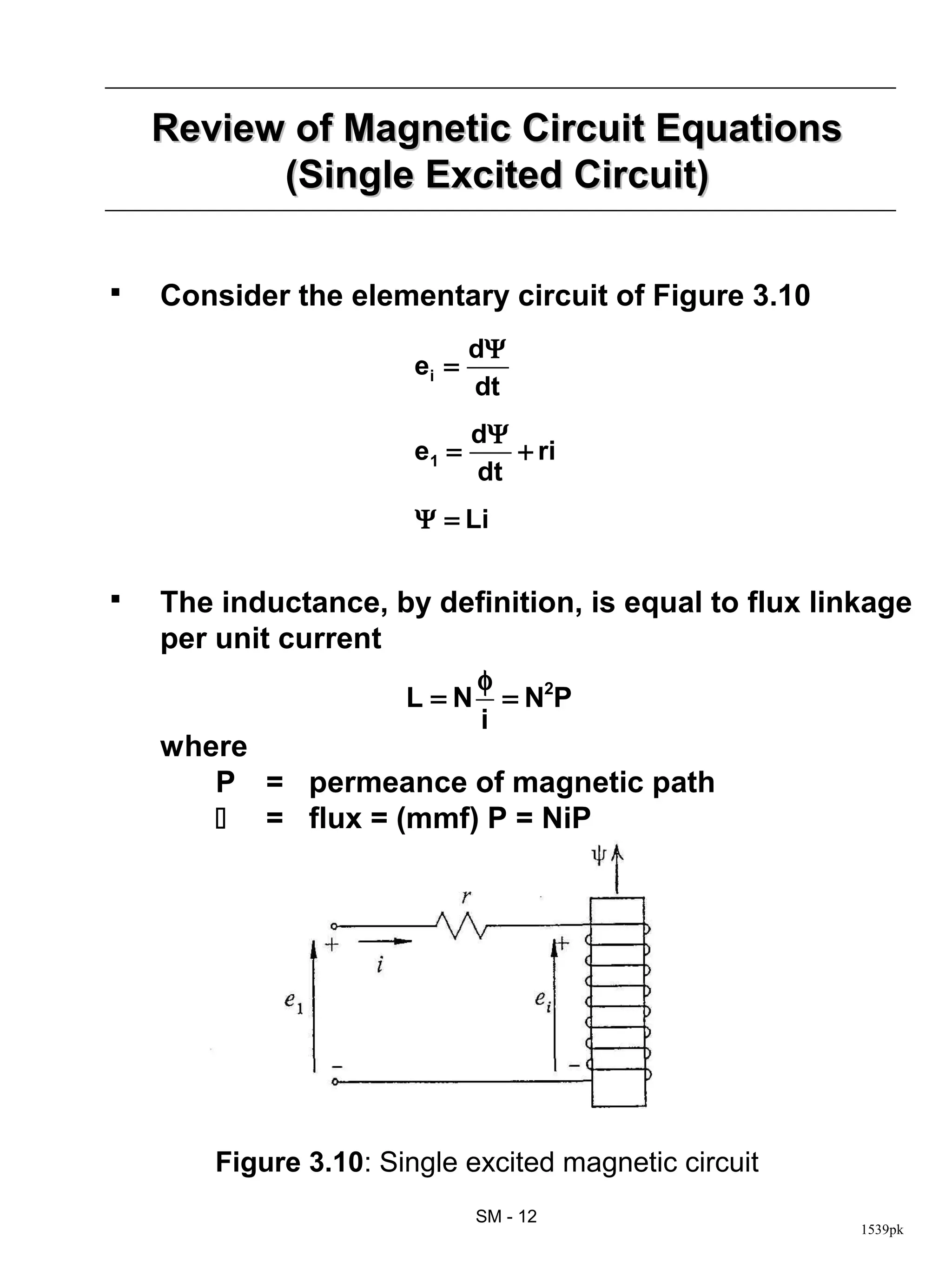
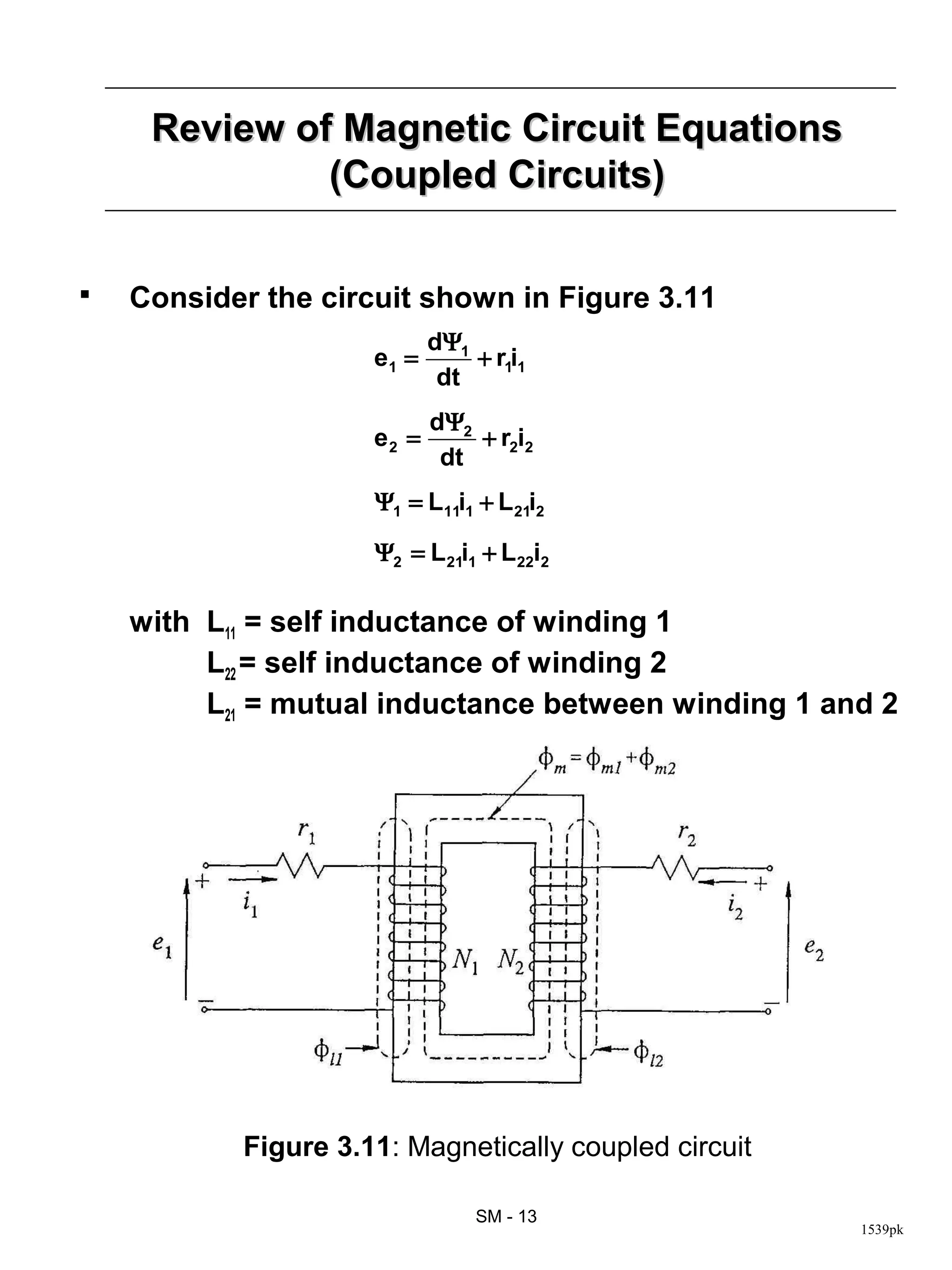
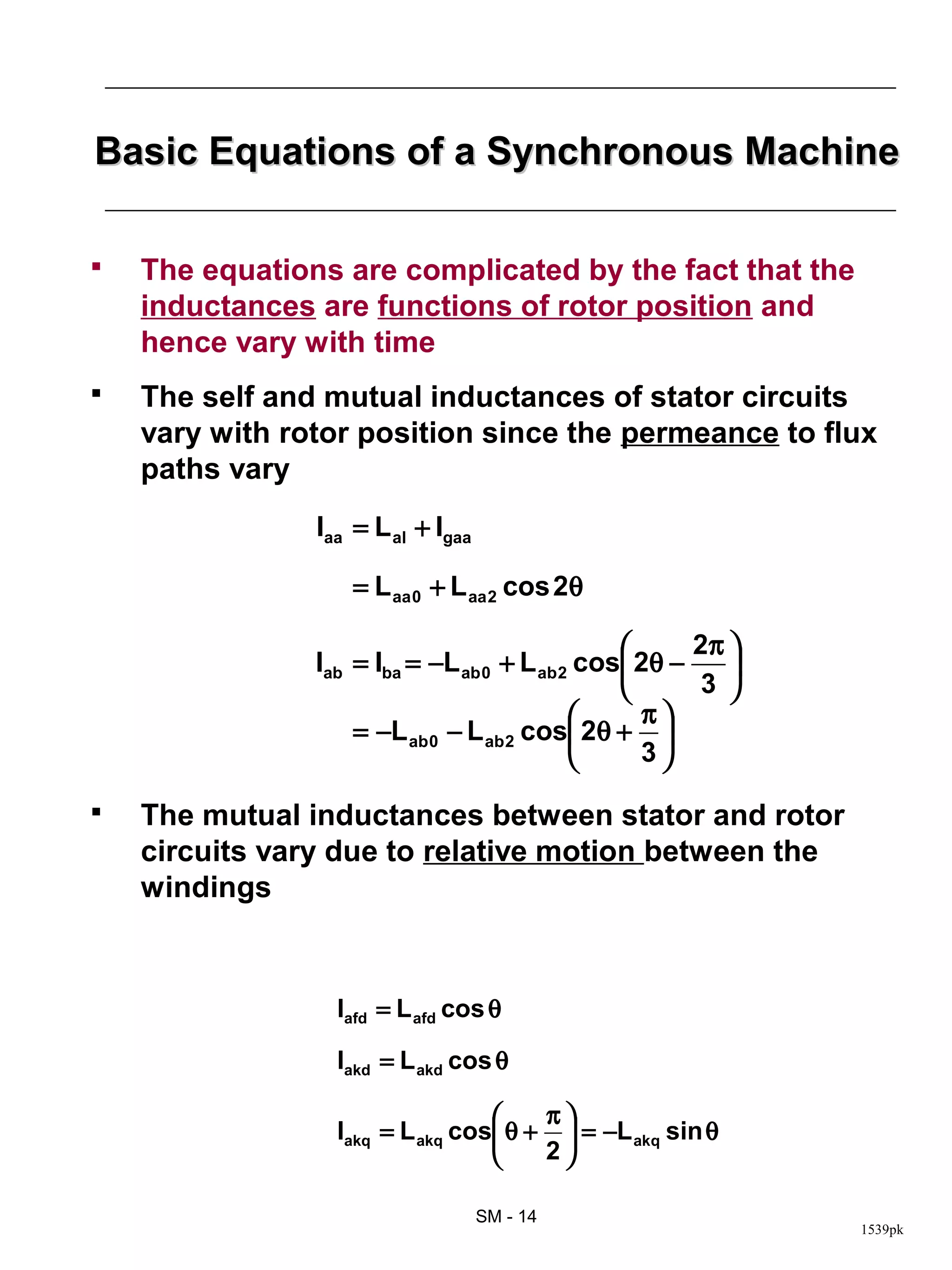
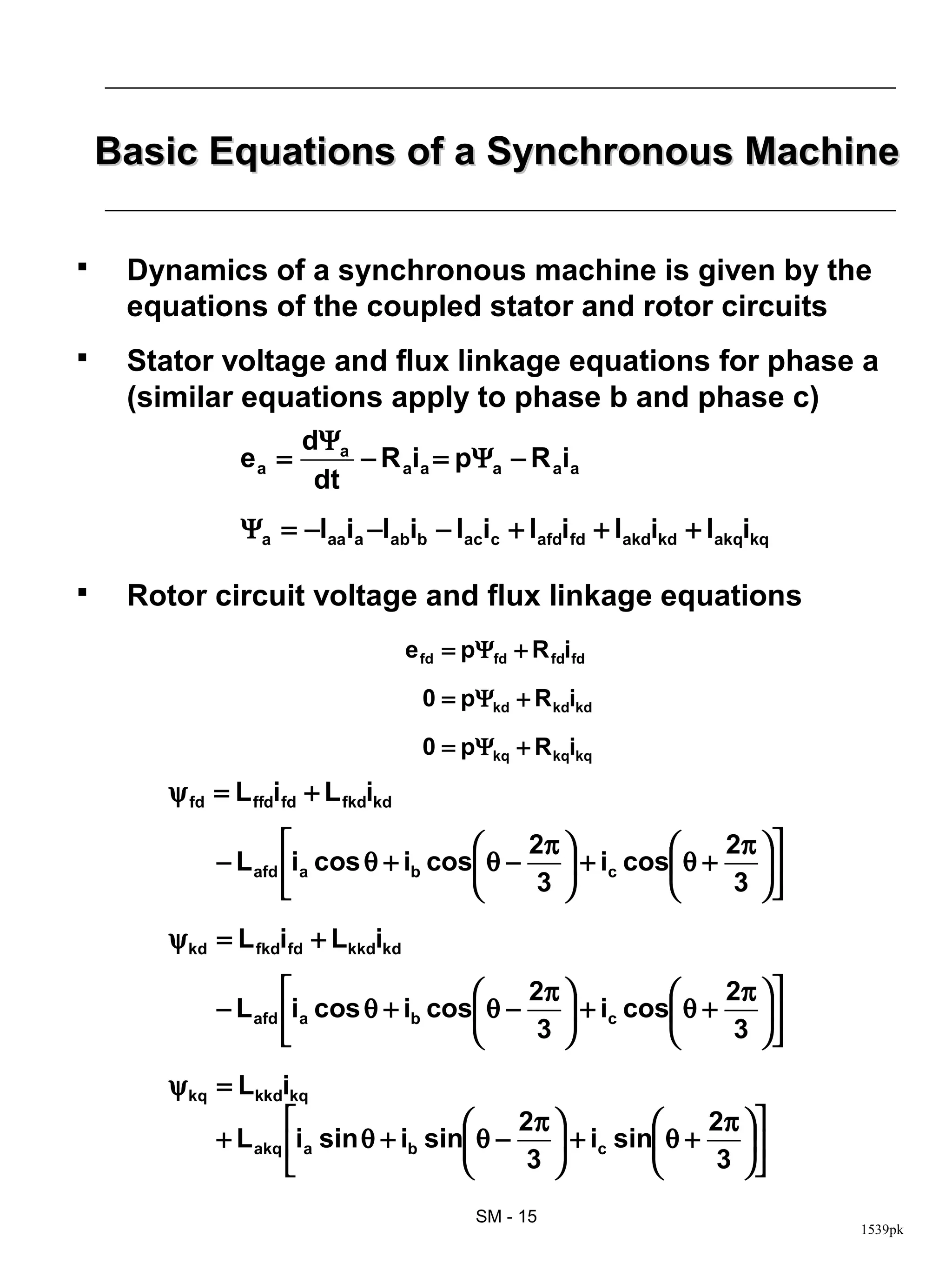
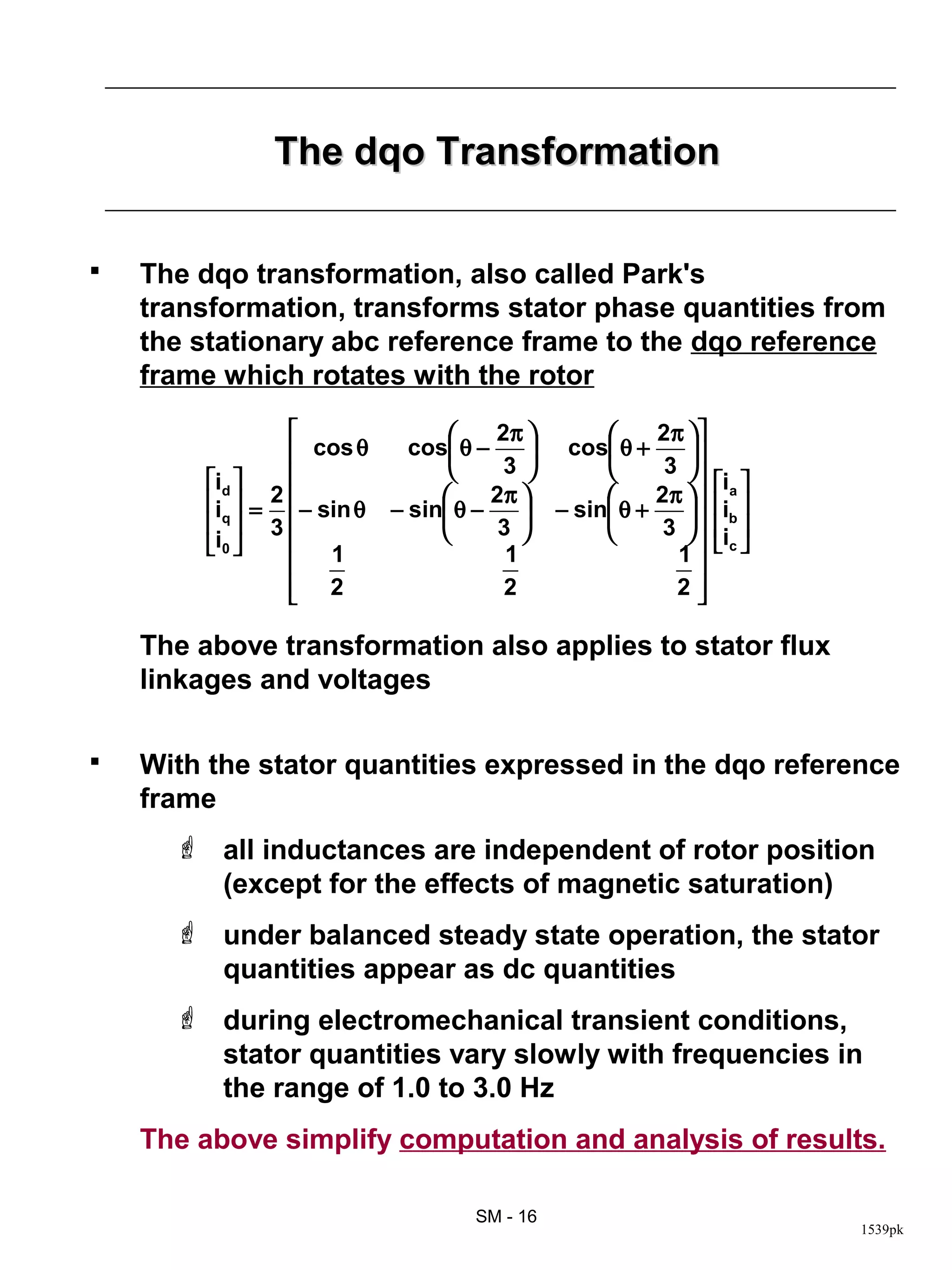
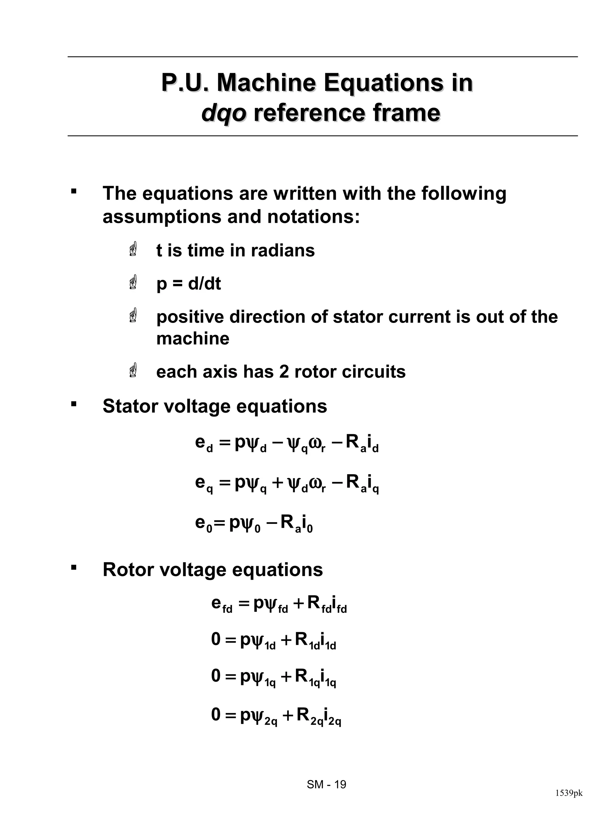
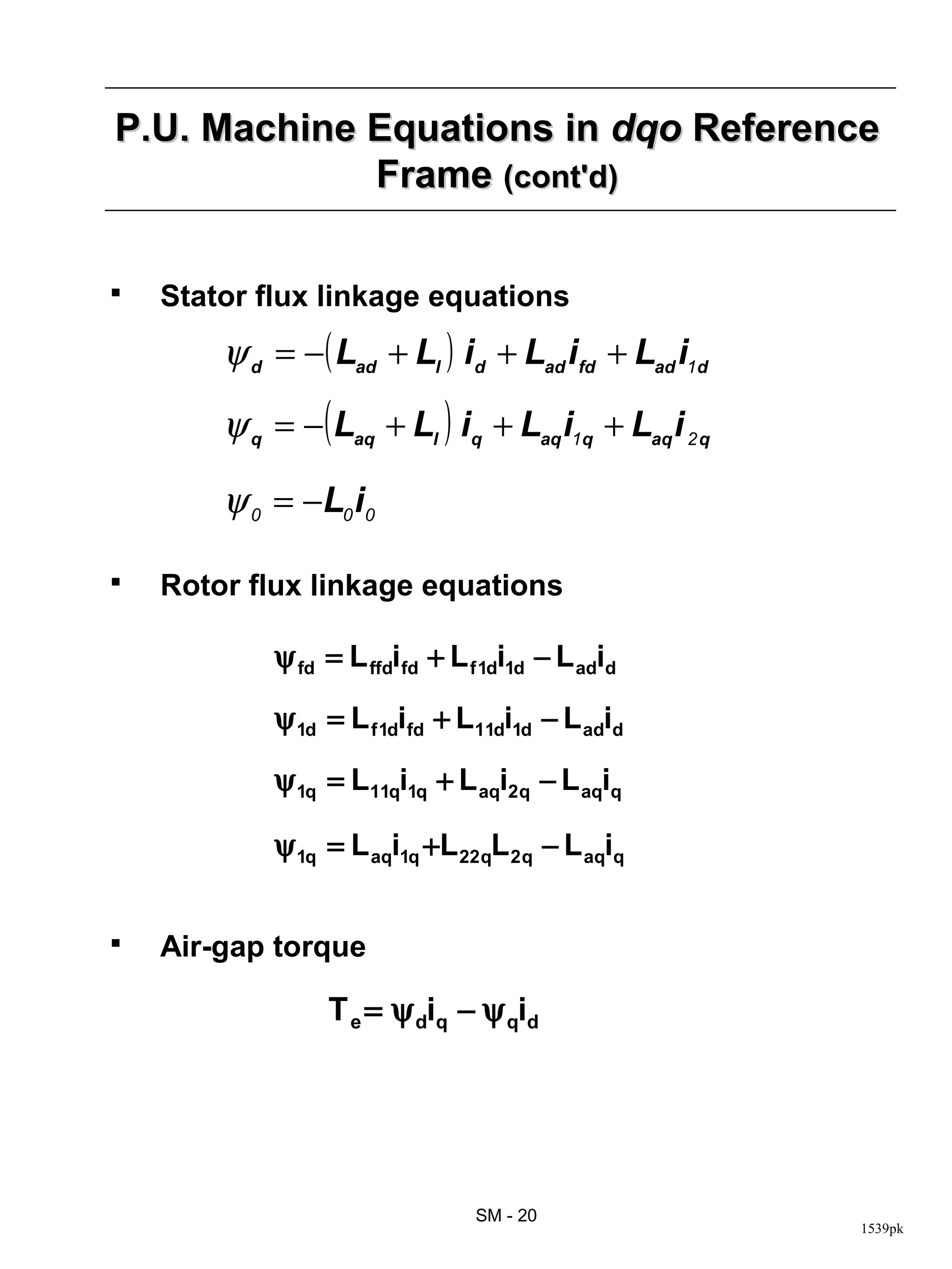
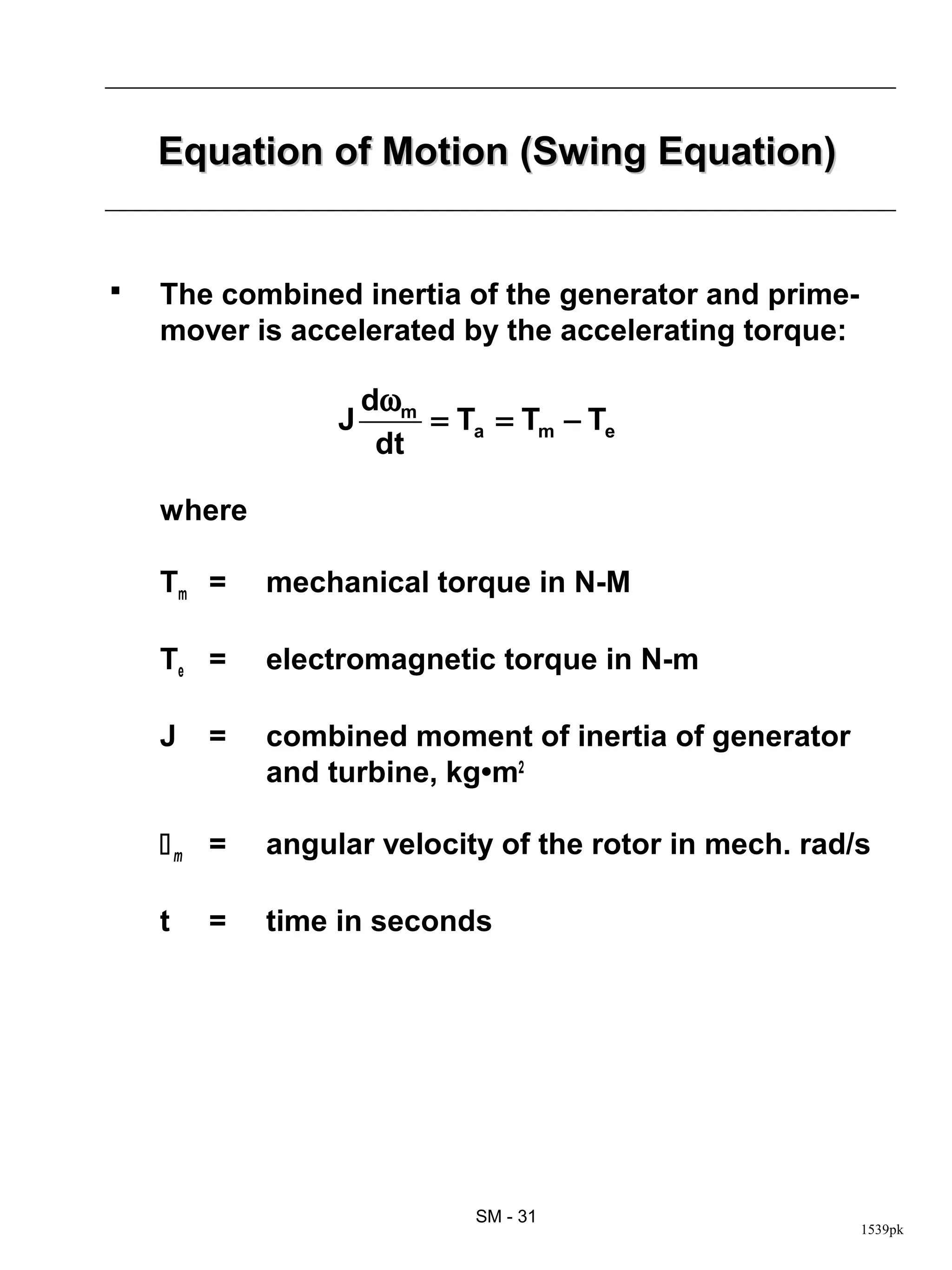
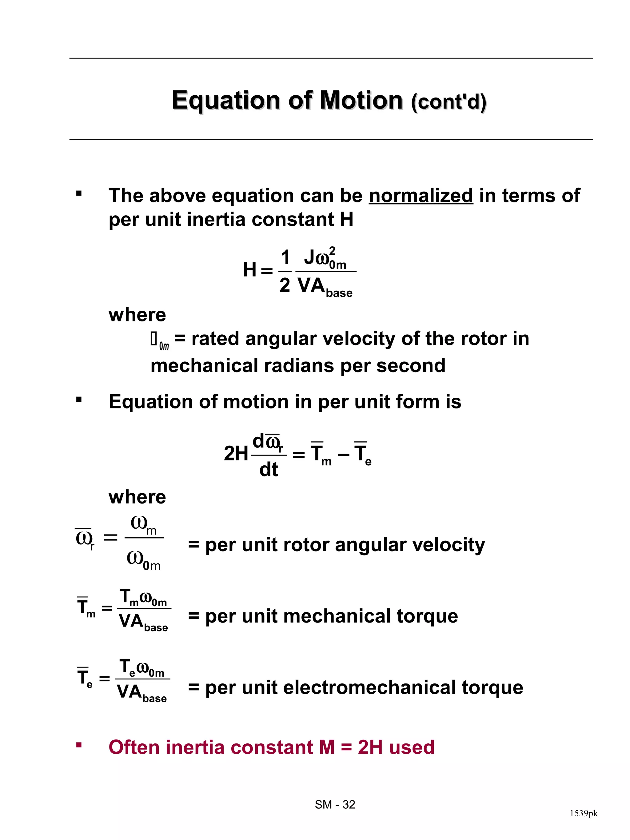
2. Their mathematical modeling using coupled circuit equations to represent stator and rotor windings.
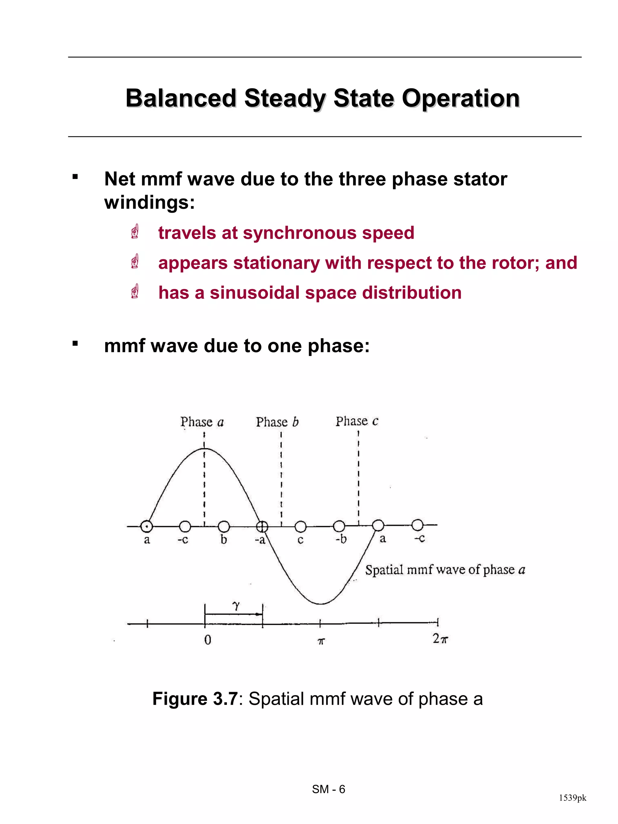
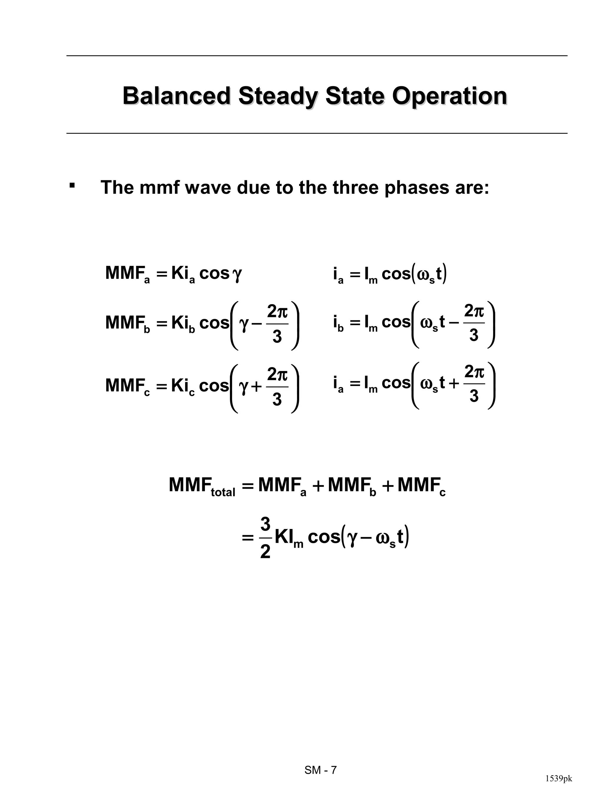
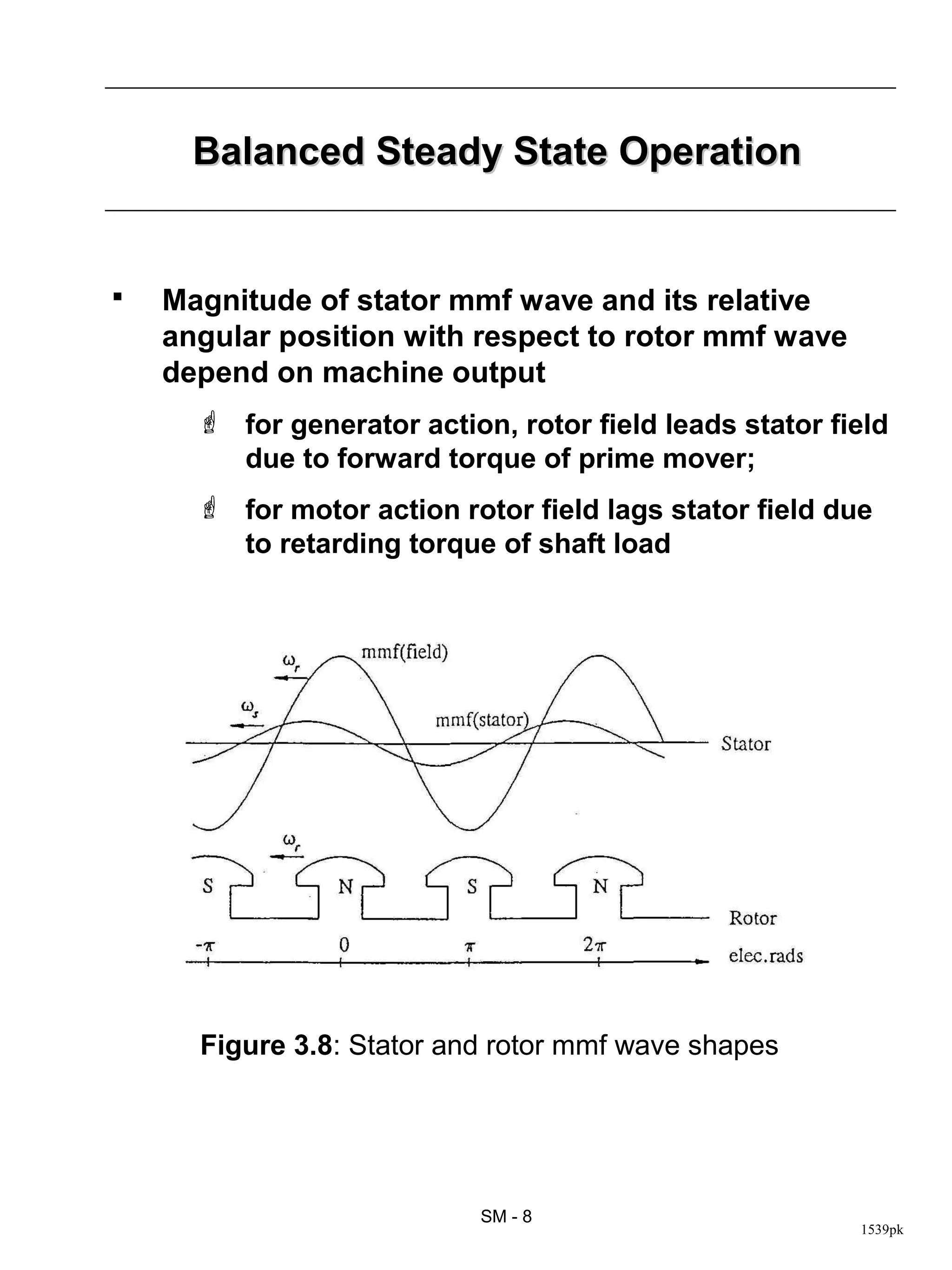
3. Their steady state operation with balanced sinusoidal stator and rotor magnetic fields.