ArUco markers are a type of fiducial marker commonly used in computer vision applications, especially because they are built into OpenCV. Since their size is known, their corners can be used with the PnP algorithm to estimate their pose in the camera frame. Additionally, ArUco markers individually encode an ID. Together, these properties make them ideal for SLAM applications.

SLAM stands for Simultaneous Localization and Mapping. This means that the system can localize itself in an environment while simultaneously building out its understanding of that environment. This project detects the position and orientation of ArUco markers in a video feed, inserts those markers into a map, and then uses various methods to optimize the estimates for both the camera and marker positions. In the video above, all markers are placed randomly; before the first frame is processed, there is no information about their positions.

Why is this important? SLAM is a fundamental problem in robotics and computer vision. Without SLAM, the small errors in odometry (wheels, IMU, etc.) accumulate and become unusable.

In the real world many robot companies, including Kiva Systems/Amazon Robotics, use a marker-based system similar to the one implemented in this repo to localize their robots and correct odometry estimates.

We can't use a normal Kalman Filter due to the non-linearity of rotations in the state vector.

Furthermore, quaternions are not vectors, so we can't use the additive updates of the EKF. Thanks to Michael from Shield AI for pointing this out to me. As such, we an MEKF in parallel for orientation. You can find a discussion of it in NASA's Navigation Filter Best Practices as well as a great, simple explanation by Matthew Hampsey here [4][5].

The key components of the Extended Kalman Filter are as follows:

• State Vector: the 3D pose (tanslation, accumulation quaternion, and a small-angle error vector) of the camera, along with the 3D position of each ArUco marker (all in the map frame):

  • camera:
    • $x_{cam}, y_{cam}, z_{cam}, qw_{cam}, qx_{cam}, qy_{cam}, qz_{cam}, ex_{cam}, ey_{cam}, ez_{cam}$
  • marker $i$:
    • $x_{mi}, y_{mi}, z_{mi}$
  • Putting the components together, the state vector will have be $3n + 10$ dimensions, for $n$ landmarks

• Measurement Vector: the 3D position of each ArUco marker in the camera frame:

  • ${}^{cam}x_{mi},{}^{cam}y_{mi},{}^{cam}z_{mi}$

• State Transition: For the motion model, we use a moving average of the last $n$ displacements to predict the camera's position motion. Since markers are static, we do not update their state:

  • $X_{k|k-1} = X_{k-1|k-1} + \frac{X_{k-1|k-1} - X_{k-n|k-n}}{n}$

• Measurement Model: in order to model what we will measure, we get the displacement between the landmark and the camera positions ($X$), and then rotate it to put it in the camera frame:

  • ${}^{cam}X_{marker} = {}^{cam}R_{map} \cdot ({}^{map}X_{marker} - {}^{map}X_{cam})$

There is an excellent explanation by Cyrill Stachniss for a similar, 2D example that can be found here [1].

python3 -m main.run_slam --video input_video.mp4 --filter ekf

Visualization of MEKF results

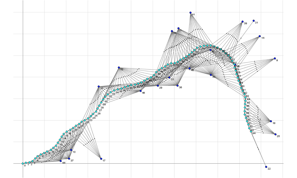
Image credit: GTSAM [2]

A factor graph optimizes the joint probability:

Where:

• $X$: the camera poses and the landmark positions.
• $Z$: the measured landmark poses in the camera frame.
• $\phi_i$: the factor that relates one camera pose to the next as well as each camera pose to the landmark that were seen at that time.

In other words, we can estimate the camera and landmark positions by optimizing the posterior probability.

The factor graph does not currently use a motion model; it simply uses the last position with a large uncertainty. I tried the motion model, but there was a large instability.

My implementation leverages GTSAM with the ISAM2 solver, following the postulation above. It reconstructs the graph at each timestep, maintaining conciseness while also accounting for both the local environment and historical constraints.

python3 -m main.run_slam --video input_video.mp4 --filter factorgraph

Visualization of online Factor Graph Results

Due to possible ambiguities in ArUco orientation estimation, only marker positions are used (hence why they are represented as points). These orientation ambiguities can be seen in the video (z axis flipping) and are discussed more thoroughly in this OpenCV github issue. In the future, I may opt to use the stable x and y dimensions as part of the state for better results.

sudo apt-get install mesa-utils libglew-dev
git clone --recursive https://github.com/yishaiSilver/aruco-slam.git
cd aruco-slam
pip install -r requirements.txt
cd thirdparty/pangolin
mkdir build
cd build
cmake .. -DPython_EXECUTABLE=`which python` -DBUILD_PANGOLIN_FFMPEG=OFF
make -j8
cd ../..
python pangolin_setup.py install
cd filterpy
python setup.py install
cd ../..

Please ensure that you have properly calibrated your camera.

.
├── input_video.mp4                  # Input video
├── main
│   ├── run_offline.py               # Script to run async factor graph SLAM
│   └── run_slam.py                  # Script to run live SLAM
├── calibration
│   ├── camera_matrix.npy            # Camera intrinsic matrix
│   ├── charuco_calibration.py       # Script to calibrate camera using images
│   ├── dist_coeffs.npy              # Camera distortion coefficients
│   └── images                       # Contains ChArUco-board calibration images
├── filters
│   ├── base_filter.py               # Base class, marker detection, map saving/loading
│   ├── extended_kalman_filter.py    # MEKF implementation
│   ├── ekf_with_rotations.py        # Same as above, but uses landmark orientations.
│   └── factor_graph.py              # Factor graph implementation
├── thirdparty
│   ├── pangolin/                    # Pangolin library for 3D visualization
│   └── pangolin_setup.py            # Custom setup script
├── viewers
│   ├── viewer_2d.py                 # Viewer/Saver for 2D image
│   └── viewer_3d.py                 # pangolin-based 3D viewer/saver
└── outputs
    ├── images
    │   ├── create_output_gif.sh     # Bash script to combine videos, convert to gif
    │   ├── output_2d.mp4            # 2D video (cv2 frame)
    │   ├── output_3d.mp4            # 3D video (pangolin frame)
    │   ├── combined.mp4             # Combined video of 2D and 3D outputs
    │   ├── ekf.gif                  # EKF results (additive quaternion update)
    │   ├── mekf.gif                 # EKF results (multiplicative update)
    │   ├── factorgraph.gif          # Factor graph results
    │   └── pangolin.png             # Pangolin screenshot (single frame for video)
    ├── map.txt                      # Saved map/landmark locations
    ├── trajectory.txt               # TUM format trajectory file
    └── trajectory_writer.py         # Creates the above trajectory.txt

• ArUco Detection, Pose Estimation
• Moving Average Motion Model (EKF)
• Filters All The Way Down Motion Model
• EKF
• Non-Additive Quaternions in EKF (MEKF)
• UKF
• Factor Graph
• Particle Filter
• 3D Visualization
• Map Saving
• Map Loading
• Trajectory Saving
• Partial, Stable Angle State for Landmarks

Nice To haves:

• Ground Truth Comparison
• Duplicate Marker ID Handling
• Non-Static Landmark Tracking
• Orientation Ambiguity Resolution
• ROS Node

[1] Cyrill Stachniss. (2020, October 2). EKF-SLAM (Cyrill Stachniss). YouTube. https://www.youtube.com/watch?v=X30sEgIws0g

[2] Dellaert, F., & GTSAM Contributors. (2022, May). borglab/gtsam (Version 4.2a8) [Software]. Georgia Tech Borg Lab. https://doi.org/10.5281/zenodo.5794541

[3] uoip. (2018, January 23). Pangolin. GitHub. Retrieved December 6, 2024, from https://github.com/uoip/pangolin

[4] Carpenter, J. R., & D’souza, C. N. (2018). Navigation filter best practices (No. NF1676L-29886).

[5] Hampsey, Matthew. “The Multiplicative Extended Kalman Filter.” Github.io, 2020, https://matthewhampsey.github.io/blog/2020/07/18/mekf. Accessed 6 Feb. 2025.