It’s time for another review for books I read this year (previously: 2024, 2022). According to my GoodReads, I read 27 books this year. Here are some highlights:
The Demon-Haunted World

I started the year with Carl Sagan’s The Demon-Haunted World, as some kind of antidote to current / coming events. I last read this in about 2010, and held it in very high regard. I still do, but Carl comes off as a bit of a fuddy duddy at times (especially when talking about “the youth” today / in the 1990s). That’s not to say that he’s wrong about where society has gone (quiet the opposite), but it as a kind of tone. If you’re interested in an introduction to skepticism, I’d probably recommend the Skeptic’s Guide to the Universe.
Pachinko

Next up was Pachinko, which had been on my list for a while but a friend’s recommendation pushed it to the top. The writing is top-notch and the characters (and the hardship the author threw at them) are still with me 11 months later.
That same friend recommend The House in the Cerulean Sea, which I read this year. I also liked it too, but not enough to rush out and read the sequel.
The Mercy of Gods

This is a new series from the authors behind The Expanse, but the setting and tone are completely different. The feelings that have stuck with me the most are the bleakness and how people survive in desperate times. Not the most uplifting stuff, but an enjoyable (or at least entertaining) read. I’m looking forward to reading more in the series when they come out.
Sailing Alone around the World

This book is a gem, and got my only 5-star of the year (aside from a re-read of another 5-star). I’d recommend it to anyone, even if you aren’t into sailing. Slocum tells the story of the first (recorded) single-handed circumnavigation of the world, which he made aboard the Spray starting in 1895. He’s an incredible writer: both in clarity and style. I loved the understated humor sprinkled throughput.
And his descriptions of the people he met along the way was surprisingly not racist, and maybe even progressive for the time. He managed to avoid the “noble savage” trope entirely. And for the most part he avoided casting any non-American / non-Europeans as “savages” of any kind (aside from the indigenous people in Tierra del Fuego who, admittedly, did try to kill him).
This is available on Project Gutenberg. Check it out!
Service Model

A fantastic little story. It took me a little while to realize that it’s actually a (dark) comedy, but once I did I was along for the ride.
I won’t spoil much it but there’s a small part that tech people / computer programmers will find entertaining. A character used the term “bits” in a couple places where I thought they should have used “bytes”. I assumed that the author (Adrian Tchaikovsky) had just made a small mistake, but no: he knew exactly what he was doing.
Nonfiction

A couple of economics books slipped into my non-fiction reading this year. First was The Price of Peace: Money, Democracy, and the Life of John Maynard Keynes by Zachary D. Carter (audiobook). Reading Keynes and commentary on Keynesian economics was a big part of my undergraduate education. Robert Skidelsky’s three-volume John Maynard Keynes is still my high-watermark for biographies.
This book gave a shorter and more modern overview of Keynes, both his life and economics (which really are inseparable).
In a similar vein, I listened to Trade Wars Are Class Wars. I can’t remember now who I got this recommendation from. I don’t remember much of it.
In the “Boating non-fiction” sub-sub-genera, I had two entries (I guess Sailing Alone around the World goes here too, but it’s so good it gets its own section).
- Into the Raging Sea by Rachel Slade: A fascinating look at the disaster that sank the container ship El Faro in the Caribbean (in 2015, so it’s not ancient history!). I won’t spoil anything, but it really is like a slow-motion train wreck. Slade does a great job telling the story.
- Sailing Smart by Buddy Melges and Charles Mason. I’ve been sailing on a Melges boat and I’m from the Midwest (Buddy is from Wisconsin) so this was like catnip to me. This was part auto-biography, part sail-racing tips. The biography part feels like pretty much any biography from a successful person (i.e. selecting on the dependant variable). I’m not a good enough sailor to judge the sail-racing tips. But it was a quick read.
Newsletters
It’s not books, but I did read every edition of a couple newsletters:
- Money Stuff by Matt Levine. And the Money Stuff podcast he hosts (with Katie Greifeld) is consistently a highlight of my week (RIP Friend of the Show Bill Ackman).
- One First by Steve Vladeck. This is useful for keeping up to date with legal news, especially things around the Supreme Court. But even more valuable is Steve’s analysis.
Hodgepodge
A few quick thoughts on a handful of books.
- A Psalm for the Wild Built, by Becky Chambers: The second Becky Chambers book I’ve read. She’s great. The actual story didn’t do much for me, but the interesting characters moving through an interesting world more than made up for that.
- To shape a Dragon’s Breath, by Moniquill Blackgoose (audiobook). I enjoyed it.
- Murderbot (again). I haven’t watched the TV show, but I re-read all the books when I was in a bit of a slump and needed something light. ART and Murderbot are the best.
- The Overstory by Richard Powers. I stopped reading this a few years ago after a certain character had a certain accident that just felt… unearned, about halfway through the book. I probably should have kept reading but couldn’t. Anyway, I picked up the audiobook and finished it off. It is a great book, but parts of it were a slog to get through.
- No Country for Old Men, by Cormac McCarthy. The Blank Check podcast covered the Coen Brothers this year so I picked up No Country. For me it’s not quite at the level of The Road but it’s still great.
- Mythos by Stephen Fry (audiobook). I highly recommend the audiobook for this one, since Stephen Fry narrates it himself. I never took a Greek History / civilization course in college, but this seemed like a really good overview.
- Endymion by Dan Simmons. This was a bit of a letdown after the first two parts of the Hyperion Cantos (which are just masterpieces). Still fun, but I haven’t moved on to the next book yet.
- A Little Hatred by Joe Abercrombie. This was a strangely easy, flowing read about a pretty awful world.
- The Adventures of Amina Al-Sirafi by Shannon Chakraborty. This book ruled. Amina rules.
- Shards of Earth by Adrian Tchaikovsky. Not my favorite Tchaikovsky, but still interesting.
- Cloud Cuckoo Land by Anthony Doerr. This was a re-read for me, after I recommended it to some friends. I felt bad for accidentally recommending a 600 page book (the downside of e-readers: you don’t appreciate how long a book is). I just love the characters, the story, the message, everything.
This post gives detailed background to my PyData Global talk, “GPU-Accelerated Zarr” (slides, video). It deliberately gets into the weeds, but I will try to provide some background for people who are new to Zarr, GPUs, or both.
The first takeaway is that zarr-python natively supports
NVIDIA GPUs. With a one-line zarr.config.enable_gpu() you can configure zarr
to return CuPy arrays, which reside on your GPU:
>>> import zarr
>>> zarr.config.enable_gpu()
>>> z = zarr.open_array("path/to/store.zarr", mode="r")
>>> type(z[:])
cupy.ndarray
The second takeaway, and the main focus of this post, is that that simple one-liner leaves performance on the table. It depends a bit on your workload, but I’d claim that Zarr’s data loading pipeline shouldn’t ever be the bottleneck. Achieving maximum throughput today requires some care to ensure that the system’s resources are used efficiently. I’m hopeful that we can improve the libraries to do the right thing in more situations.
This post pairs nicely with Earthmover’s I/O-Maxing Tensors in the Cloud post, which showed that network and object storage service (e.g. S3) also shouldn’t be a bottleneck in most workloads. Ideally, your actual computation is where the majority of time is spent, and the I/O pipeline just gets out of your way.
Some background
I imagine that some people reading this have experience with Zarr but not GPUs, or vice versa. Feel free to skip the sections you’re familiar with, and meet up with us at the Speed of Light section.
Zarr Background for GPU People
Zarr is many things, but today we’ll focus on Zarr as the storage
format for n-dimensional arrays. Instead of tabular data, which you might store
in a columnar format like Apache Parquet, you’re working with data that fits
things like xarray’s data model: everything is an n-dimensional array with
metadata. For example, 3-d array measuring forecasts for a temperature field
with dimensions (x, y, time).

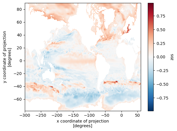
Zarr is commonly used in many domains including microscopy, genomics, remote sensing, and climate / weather modeling. It works well with both local file systems and remote cloud object storage. High-level libraries like xarray can use zarr as a storage format:
# https://tutorial.xarray.dev/intermediate/remote_data/cmip6-cloud.html
>>> ds = xr.open_zarr(
...     "gs://cmip6/CMIP6/ScenarioMIP/NOAA-GFDL/...",
...     consolidated=True,
... )
>>> zos_2015jan = ds.zos.sel(time="2015-01-16")
>>> zos_2100dec = ds.zos.sel(time="2100-12-16")
>>> sealevelchange = zos_2100dec - zos_2015jan
>>> sealevelchange.plot.imshow()
xarray knows how to translate the high-level slicing like time="2015-01-16" to
the lower level slicing of a Zarr array, and Zarr knows how to translate
positional slices in the large n-dimensional array to files / objects in
storage. This diagram shows the structure of a Zarr store:
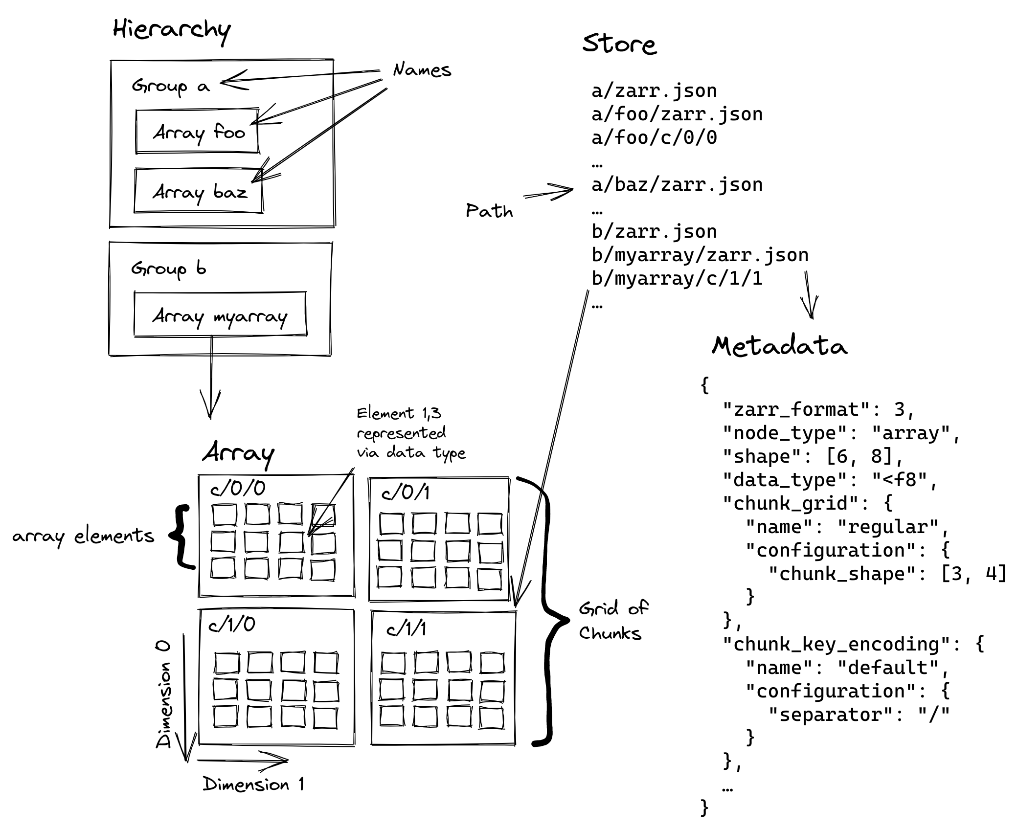
The large logical array is split into one or more chunks along one or more dimensions. The chunks are then compressed and stored to disk, which lowers storage costs and can improve read and write performance (it might be faster to read fewer bytes, even if you have to spend time decompressing them).
Zarr’s sharding codec is especially important for GPUs. This makes it possible to store many chunks in the same file (a file on disk, or an object in object storage). We call the collection of chunks a shard, and the shard is what’s actually written to disk.

Multiple chunks are (independently) compressed, concatenated, and stored into the same file / object. We’ll discuss this more when we talk about performance, but the key thing sharding provides is amortizing some constant costs (opening a file, checking its length, etc.) over many chunks, which can be operated on in parallel (which is great news for GPUs).
For now, just note that we’ll be dealing with various levels of Zarr’s hierarchy:
- Arrays: the logical n-dimensional array
- Shards: the file on disk / object in object storage, which contains many chunks concatenated together
- Chunks: the smallest unit we can read (since it must be decompressed to interpret the bytes correctly)
GPU Background for Zarr People
GPUs are massively parallel processors: they excel when you can apply the same problem to a big batch of data. This works well for video games, ML / AI workloads, and data science / data analysis applications.
(NVIDIA) GPUs execute “kernels”, which are essentially functions that run on GPU data. Today, we won’t be discussing how to author a compute kernel. We’ll be using existing kernels (from libraries like nvcomp, CuPy, and CCCL). Instead, we’ll be worried about higher-level things like memory allocations, data movement, and concurrency
Many (though not all) GPU architectures have dedicated GPU memory. This is separate from the regular main memory of your machine (you’ll hear the term “device” to refer to GPUs, and “host” to refer to the host operating system / machine, where your program is running).
While device memory tends to be relatively fast compared to host memory (for example, it might have >3.3 TB/s from the GPU’s memory to its compute cores), it’s moving data between host and device memory is relatively slow (perhaps just 128 GB/s over PCIe). It also tends to be relatively small (an NVIDIA H100 has 80-94GB of GPU memory; newer generations have more, but still GPU memory is precious when processing large datasets). All this means we need to be careful with memory, both how we allocate and deallocate memory and how we move data between the host and device.
In GPU programming, keeping the GPU busy is necessary (but not sufficient!) to achieve good performance. We’ll use GPU utilization, the percent of time (over some window) when the GPU was busy executing some kernel, as a rough measure of how well we’re doing.
One way to achieve high GPU utilization is to queue up work for the GPU to do. The GPU is a device, a coprocessor, onto which your host program offloads work. As much as possible, we’ll have our Python program just do orchestration, leaving the heavy computation to the GPU. Doing this well requires your host program to not slow down the (very fast) GPU.
In some sense, you want your Python program to be “ahead” of the GPU. If you wait to submit your next computation until some data is ready on the GPU, or some previous computation is completed, you’ll inevitably have some time gap when your GPU is idle. Sometimes this is inevitable, but with a bit of care we’ll be able to make our Zarr example perform well.
My Cloud Native Geospatial Conference post touched on this under Pipelining. This program waits to schedule the computation until the CPU is done reading the data, and so doesn’t achieve high throughput:

This second program queues up plenty of work to do, and so achieves higher throughput:

For this example, we’ll use a single threaded program with multiple CUDA Streams to achieve good pipelining. CUDA streams are a way to express a sequence (a stream, if you will) of computations that must happen in order. But, crucially, you can have multiple streams active at the same time. This is nice because it frees you from having to worry too much about exactly how to schedule work on the GPU. For example, one stream of computation might heavily use the memory subsystem (to transfer data from the host to device, for example) while another stream might be using the compute cores. But you don’t have to worry about timing things so that the memory-intensive operation runs at the same time as the compute-intensive operation.
In pseudocode:
a0 = read_chunk("path/to/a", stream=stream_a)
b0 = read_chunk("path/to/b", stream=stream_b)

a1 = transform(a0, stream=stream_a)
b1 = transform(b0, stream=stream_b)
read_chunk might exercise the memory system to transfer data from the host to
the device, while transform might really hammer the compute cores.
All you need to do is “just” correctly express the relationships between the different parts of your computation (not always easy!). The GPU will take care of running things concurrently where possible.
One subtle point here: these APIs are typically non-blocking in your host
Python (or C/C++/whatever) program. read_chunk makes some CUDA API calls
internally to kick off the host to device transfer, but it doesn’t wait for that
transfer to complete. This is good, since we want our host program to be well
ahead of the GPU; we want to go to the next line and feed the GPU more work to
do.
If we actually poked the memory address where the data’s supposed to be it might
be junk. We just don’t know. If we really need to wait for some data /
computation to be completed, we can call stream.synchronize(), which forces
the host program to wait until all the computations on that stream are done.
But ideally, you don’t need that. For the typical case of launching some
CUDA kernel some some data, synchronization is unnecessary. You only need
to ensure that the computation happens on the same CUDA stream as the data
loading (like in our pseudocode example, launching each transform on
the appropriate stream), and you’re good to go.
CUDA streams do take some getting used to. You can make analogies to thread programming and to async / await, but that only gets you so far. At the end of the day they’re an extremely useful tool to have in your toolkit.
Speed of Light
When analyzing performance, it can be helpful to perform a simple “speed-of-light” analysis: given the constraints of my system, what performance (throughput, latency, whatever metric you care about) should I expect to achieve? This can combine abstract things (like a performance model for how your system operates) with practical things (what’s the sequential read throughput of my disk? What’s the clock cycle of my CPU?).
Many Zarr workloads involve (at least) three stages:
-
Reading bytes from storage (local disk or remote object storage). Your disk (for local storage) or NIC / remote storage service (for remote storage) has some throughput, which you should aim to saturate. Which bytes you need to read will be dictated in part by your application. Zarr supports reading subsets of data (with the chunk being the smallest decompressable unit). Ideally, your chunking should align with your access pattern.
-
Decompressing bytes with the Codec Pipeline. Different codecs have different throughput targets, and these can depend heavily on the data, chunk size, and hardware. We’re using the default Zstd codec in this example.
-
Your actual computation. This should ideally be the bottleneck: it’s the whole reason you’re loading all this data after all.
And if you are using a GPU, at some point you need to get the bytes from host to device memory1.
Finally, you might need to store your result. If your computation reduces the data this might be negligible. But if you’re outputting large n-dimensional arrays this can be as or more expensive than the reading.
In this case, we don’t really care about what the computation is; just something that uses the data and takes a bit of time. We’ll do a bunch of matrix multiplications because they’re pretty computationally expensive and they’re well suited to GPUs.
Notably, we won’t do any kind computation that involves data from multiple shards. They’re completely independent in this example, which makes parallelizing at the shard level much simpler.
Example Workload
This workload operates on a 1-D float32 array with the following properties:
| Level | Shape | Size (MB) | Count per parent |
|---|---|---|---|
| Chunk | (256_000,) |
1.024 | 400 chunks / shard |
| Shard | (102_400_000,) |
409.6 | 8 shards / array |
| Array | (819_200_000,) |
3,276.8 | - |
Each chunk is Zstd compressed, and the shards take about 77.5 MB on disk giving a compression ratio of about 5.3.
The fact that the array is 1-D isn’t too relevant here: zarr supports n-dimension arrays with chunking along any dimension. It does ensure that one optimization is always available when decoding bytes, because the chunks are always contiguous subsets of the shards. We’ll talk about this in detail in the Decode bytes section.
Our workload will read the data, transfer it to the GPU (if using the GPU) and perform a bunch of matrix multiplications.
Performance Summary
This example workload has been fine-tuned to make the GPU look good, and I’ve done zero tuning / optimization of the CPU implementation. Any comparisons with CPU libraries are essentially bunk, but it’s a natural question so I’ll report them anyway.
The top level summary will compare three implementations:
- zarr-python: Uses vanilla zarr-python for I/O and decoding, and NumPy for the computation.
- zarr-python GPU: Uses zarr-python’s built-in GPU support to return CuPy arrays, so the GPU is used for computation. At the moment, this still uses Numcodecs to decompress the data, which runs on the CPU. After decompression, the data is moved to the GPU for the matrix multiplication.
- Custom GPU: My custom implementation of I/O and decoding with CuPy for the computation.
| Implementation | Duration (ms) |
|---|---|
| Zarr / NumPy | 19,892 |
| Zarr / CuPy | 3,407 |
| Custom / CuPy | 478 |
You can find the code for these in my CUDA Stream Samples repository.
Please don’t take the absolute numbers, or even the relative numbers too seriously. I’ve spent zero time optimizing the Zarr/NumPy and Zarr/CuPy implementations. The important thing to take away here is that we have plenty of room for improvement. My Custom I/O pipeline just gradually removed bottlenecks as they came up, some of which apply to zarr-python’s CPU implementation as well. Follow https://github.com/zarr-developers/zarr-python/issues/2904 if you’re interested in developments.
The remainder of the post will describe, in some detail, what makes the custom implementation so fast.
Performance optimizations
Once you have the basics down (using the right data structures / algorithm, removing the most egregious overheads), speeding up a problem often involves parallelization. And you very often have multiple levels of parallelization available. Picking the right level is absolutely a skill that requires some general knowledge about performance and specific details for your problem.
In this case, we’ll operate at the shard level. This will be the maximum amount of data we need to hold in memory at any point in time (though the problem is small enough that we can operate on all the shards at the same time).
We’ll use a few techniques to get good performance in our pipeline:
- No (large) memory allocations on the critical path.
This applies to both host and device memory allocations. We’ll achieve this by preallocating all the arrays we need to process the shard. Whether or not this should be considered cheating or not is a bit debatable and a bit workload dependent. I’d argue that the most advanced, performance-sensitive workloads will process large amounts of data and so can preallocate a pool of buffers and reuse them across their unit of parallelization (shards in our case).
Regardless, if we’re doing large memory allocations after we’ve started processing a shard (either host or device allocations for the final array or for intermediates) then these allocations can quickly become the bottleneck. Pre-allocation (and reuse across shards) is an important optimization if it’s available.
- Use pinned (page-locked) memory for host buffers
Using pinned memory makes the host to device transfers much faster. More on that later.
- Use CUDA streams to overlap I/O and Computation
Our workload has a regular pattern of “read, transfer, decode, compute” on each shard. Because these exercise different parts of the GPU (transfer uses the memory subsystem, decode and compute launch kernels that run on the GPU’s cores), we can run them concurrently.
We’ll assign a CUDA stream per shard. We’ll be very careful to avoid stream / device synchronizations so that our host program schedules all the work to be done.
Throughout this, we’ll use nvtx to annotate certain ranges of code. This will make reading the Nsight Systems report easier.
Here’s a screenshot of an nsys profile, with a few important bits highlighted (open the file for a full-sized screenshot):

- Under Processes > Threads > python, you see the traces for our host program,
in this case a Python program. This will include our nvtx annotations
(
read::disk,read::transfer,read::decode, etc.) and calls to the CUDA API (e.g.cudaMemcpyAsync). These calls measure the time spent by the CPU / host program, not the GPU.

- Under Processes > CUDA HW, you’ll see the corresponding traces for GPU operations. This shows CUDA kernels (functions that run on the GPU) in light blue and memory operations (like host to device transfers) in teal.

You can download the full nsight report here and open it locally with NVIDIA Nsight Systems.
This table summarizes roughly where we spend our time on the GPU per shard (very rough, and there’s some variation across shards, especially as we start overlapping operations with CUDA streams).
| Stage | Duration (ms) | Raw Throughput (GB/s) | Effective Throughput (GB/s) |
|---|---|---|---|
| Read | 13.6 | 5.7 | 30.1 |
| Transfer | 1.5 | 51.7 | 273 |
| Decode | 45 | 1.7 | 9.1 |
| Compute | 150 | 2.7 | 2.7 |
Raw throughput measures the actual number of bytes processed per time unit,
which is the compressed size for reading, transferring, and decoding.
“Effective Throughput” uses the uncompressed number of bytes for each stage.
After decompression the actual number of bytes processed equals the uncompressed
bytes, so Compute’s raw throughput is equal to its effective throughput.
Read bytes
First, we need to load the data. In my example, I’m just using files on a local disk, though you could use remote object storage and still perform well. We’ll parallelize things at the shard level (i.e. we’re assuming that the entirety of the shard fits in GPU memory).
path = array.store_path.store.root / array.store_path.path / key

with open(path, "rb") as f, nvtx.annotate("read::disk"):
    f.readinto(host_buffer)
On my system, it takes about 13.6 ms to read the 77.5 MB, for a throughput of about 5.7 GB/s from disk (the OS probably had at least some of the pages cached). The effective throughput (uncompressed size over duration) is about 30.1 GB/s. I’ll note that I haven’t spent much effort optimizing this section.
Note that we use readinto to read the data from disk directly into the
pre-allocated host buffer: we don’t want any (large) memory allocations on the
critical path. Also, we’re using pinned memory (AKA page-locked
memory) for the host buffers. This prevents the operating system from paging the
buffers, which lets the GPU directly access that memory when copying it, no
intermediate buffers required.
And it’s worth emphasizing: this I/O is happening on the host Python program, and it is blocking. As we’ll see later, time spent doing stuff in Python is time not spent scheduling work on the GPU. We’ll need to ensure that the GPU is fed sufficient work, so let’s keep our eye on this section.
The profile report for this section is pretty boring:

Note what the GPU is doing right now: nothing! There aren’t any CUDA HW
annotations visible above the initial read::disk. At least for the very first
shard we read, the GPU is necessarily idle. But as we’ll discuss shortly,
subsequent shards are able to overlap disk I/O with CUDA operations.
This screenshot shows the profile for the second shard:

Now the GPU is busy with some other operations (decoding the chunks from the
first shard in this case, which are directly above the read::decode happening
on the host at that time). This is partly why I didn’t bother with parallelizing
the disk I/O: only one thing can be the bottleneck, and right now we’re able to
load data from disk quickly enough.
Transfer bytes
After we’ve read the bytes into memory, we schedule the host to device transfer:
with nvtx.annotate("read::transfer"), stream:
    # device_buffer is a pre-allocated cupy.ndarray
    device_buffer.set(
        host_buffer[:-index_offset].view(device_buffer.dtype), stream=stream
    )
This is where our earlier discussion on blocking vs. non-blocking APIs comes
in handy. The device_buffer.set call is not blocking, which is why it
takes only ~60 μs on the host. It only makes the CUDA API call to set up
the transfer and then immediately returns back to the Python program (to
close our context managers and then continue to the next line in our program).
The actual memory copy (which is running on the device) takes about 1.5 ms for a throughput of about 52 GB/s (this is still compressed data, so the effective throughput is even higher). Here’s the same profile I showed earlier, but now you’ll understand the context around what happens on the host (the CUDA API call to do something) and device.
![]()
I’ve added the orange lines connecting the fast cudaMemcpyAsync on the host to
the (not quite as fast) Memcpy HtoD (host to device) running on the device.
And if you look closely, you’ll see that just above that Memcpy HtoD in teal,
we’re executing a compute kernel (in light-blue). We’ll get to that in a bit,
but this show that we’re overlapping Host-to-Device transfers with compute
kernels.
Decode bytes
At this point we have (or will have, eventually) the Zstd compressed bytes in GPU memory. You might think that “decompressing a stream of bytes” doesn’t mesh well with “GPUs as massively parallel processors”. And you’d be (partially) right! We can’t really parallelize decoding within a single chunk, but we can decode all the chunks in a shard in parallel. My colleague Akshay has a nice overview of how the GPU can be used to decode many buffers in parallel.
I have no idea how to implement a Zstd decompressor, but fortunately we don’t have to. The nvCOMP library implements a bunch of GPU-accelerated compression and decompression routines, including Zstd. It provides C, C++, and Python APIs. A quick note: this example is using a custom wrapper around nvcomp’s C API. This works around a couple issues with nvcomp’s Python bindings.
- At the moment, accessing an attribute on the decompressed array returned by nvcomp causes a “stream synchronization”. This forces essentially blocks the host program from progressing until the GPU has caught up, which we’d like to avoid. We need to issue compute instructions still, and we’d ideally move on to the next shard!
- We’d like full control over all the memory allocations, including the ability to preallocate the output buffers that the arrays should be decompressed into. This is possible with the C API, but not (yet) the Python API.
My custom wrapper is not at all robust, well designed, etc. It’s just enough to work for this demo. Don’t use it! Use the official Python bindings, and reach out to me or the nvcomp team if you run into any issues. But here’s the basic idea in code:
zstd_codec = ZstdCodec(stream=stream)
# get a list of arrays, each of which is a view into the original device buffer
# `device_buffer` is stream-ordered on `stream`,
# so `device_arrays` are all stream-ordered on `stream`
device_arrays = [
    device_buffer[offset : offset + size] for offset, size in index
]
with nvtx.annotate("read::decode"):
    zstd_codec.decode_batch(device_arrays, out=out_chunks)

# and now `out` is stream-ordered on `stream`
The zstd_codec.decode_batch call takes about 2.4 ms on my machine. Again
this just schedules the decompression call.
The actual decompression takes about 25-45 ms, for a throughput of about roughly 1.7 GB/s.
Again, we’ve pre-allocated the out ndarray, however this is not always
possible. Zarr allows chunking over arbitrary dimensions, but we’ve assumed
that the chunks are contiguous slices of the output array2. If
your chunks aren’t contiguous slices of the output array, you’ll need to
decode into an intermediate buffer and then perform some memory copies
into the output buffer.
Anyway, all this is to say that decompression isn’t our bottleneck. And this is despite decompression competing for GPU cores with the computation. The newer NVIDIA Blackwell Architecture includes a dedicated Decompression Engine which improves the decompression throughput even more.
And for those curious, a brief experiment without compression is about twice as slow on the GPU as the version with compression, though I didn’t investigate it deeply.
Computation
This example is primarily focused on the data loading portion of a Zarr workload, so the computation is secondary. I just threw in a bunch of matrix multiplications / reductions (which GPUs tend to do quickly).
But while the specific computation is unimportant, there are some characteristics to consider about your computation, it should take some non-negligible amount of time, such it’s worthwhile moving the data from the host to the device for the computation (and moving the result back to the host).
The key thing we care about here is overlapping host to device copies with compute, so that the GPU isn’t sitting around waiting for data. Note how the teal Host to Device Copy is running at the same time as the matrix multiplication from the previous shard:

And at this point, you can start analyzing GPU metrics if you still need to squeeze additional performance out of your pipeline.

But I think that’s enough for now.
Summary
One takeaway here is that GPUs are fast, which, sure. A slightly more interesting takeaway is that GPUs can be extremely fast, but achieving that takes some care.
In this workload my custom pipeline achieved high throughput by
- Being very careful with memory allocations and data movement.
- Using pinned host memory to speed up the one host to device transfer per shard
- Use nvcomp and Zarr shards to parallelize decoding many chunks on the GPU
- Use CUDA streams to express our workloads’ shard-level parallelism, so that we can overlap host I/O, host-to-device copies, kernel launches and kernel execution.
I’m hopeful that we can optimize the codec pipeline and memory handling in zarr-python to close the gap between what it provides and my custom, hand-optimized implementation (0.5s). But doing that in a general purpose library will require even more thought and care than my hacky implementation.
If you’ve made it this far, congrats. Reach out if you have any feedback, either directly or on the Zarr discussions board.
-
NVIDIA does have GPU Direct Storage which offers a way to read directly from storage to the device, bypassing the host (OS and memory system) entirely. I haven’t tried using that yet. ↩︎
-
Explaining that optimization in more detail. We need the chunks to be contiguous in the shard. Consider this shard, with the letters indicating the chunks:
| a a a a |
| b b b b |
| c c c c |
| d d d d |
In C-contiguous order, that can be stored as:
| a a a a b b b b c c c c d d d d|i.e. all of the
a’s are together in a contiguous chunk. That means we can tell nvcomp to write its output at this memory address and it’ll work out fine. Likewise forb, just offset by some amount, and so on for the other chunks.However, this chunking is not amenable to this optimization because the chunks aren’t contiguous in the shard:
| a a b b |
| a a b b |
| c c d d |
| c c d d |
Maybe someone smarter than me could pull off something with stride tricks. But for now, note that the ability to preallocate the output array might not always be an option.
That’s not necessarily a deal-killer: you’ll just need a temporary buffer for the decompressed output and an extra memcpy per chunk into the output shard. ↩︎
Last weekend I had the chance to sail in the 2025 Corn Coast Regatta. I had such a great time that I had to jot down my thoughts before they fade. This post is mostly for (future) me. We’ll return to our regularly scheduled programming in a future post. I have a post on Zarr performance cooking.
First, some context: in August I attended the Saylorville Yatch Club Sailing School Adult Small Boat class. This is a 3-day course that mixes some time in the classroom learning the theory and jargon (so much jargon!) with a bunch of time on the water. I had a bit of experience from sailing on summer weekends with my family growing up, but I wanted to learn more before going out on my own.
We were thrown in on the deep end, thanks to how breezy Saturday and Sunday. Too breezy for sailors as green as us, as it turns out. At least we got to practice capsize recovery a bunch.

Our instructor, Nick, was great. He’s knowledgeable, passionate about sailing, and invested in our success. If you’re near the area and at all interested in sailing, I’d recommend taking the course (and other clubs offer their own courses).
After the course, Nick was extremely generous. He invited us out for the Wednesday night beer can races the Yatch Club hosts, on his Melges 24. This was quite the step up from the Precision 185 we sailed during the class.
I hadn’t done any racing before and was immediately hooked. During the races, I was mostly just rail meat (“hiking” out on the lifelines to keep the boat from heeling over as we go upwind) and tried to not get in the way. But afterwards Nick was adamant about everyone getting to try the other jobs on the boat. Trimming the spinnaker (a very big sail that’s exclusively used going downwind) was awesome. There aren’t any winches on the Melges 24, so you directly feel the wind powering the boat when you’re flying the spinnaker.
Which brings us to last weekend. Nick was looking for some people to crew during the regatta, and we ended with Nick (driving), me (hiking upwind and flying the spin downwind), and a few other sailing school alumni on the boat. We started early on Saturday, rigging the special black carbon fiber sails Nick uses for regattas.

After a quick captains’ meeting we launched the boat and got ready to sail. Saturday was a series of short-distance buoy races. We ended up getting four races in, and our boat took second in each race to a Viper 640 sailed by a very experienced and talented father / son crew1. A couple of races came down to the wire, and we might have won the third race if I hadn’t messed up our last gybe by grabbing the spinnaker sheet on the wrong side of the block and fouling everything up. Oops.
Sunday was the distance race. We started in about the middle of the lake, sailed a very wet 2 – 2.5 miles upwind (southeast) to the Saylorville Dam, followed by a long 4 – 5 mile downwind leg to the bridge on the north side of the lake, and finished with a ~2 mile leg to the end. The wind really picked up on Sunday, blowing ~15 kts with gusts up to 20–25 kts. As we neared the upwind mark, we had some discussions about whether or not to fly the spinnaker. That’s a lot of wind for a crew as inexperienced as we were (we’d only had one practice and the previous days’ races together). We took our time rounding the mark and eventually decided to set it. Nick took things easy on us, and overall things went well. We about went over twice (probably my fault; I was exhausted by the time we got 1/2 down the course) but our jib trimmer bailed us out both times just like we talked about in our pre-race talk. It sounds like even the Viper went over, so I don’t feel too bad.
Our team had really gelled by the end of the regatta. Crossing the finish line in first place was exhilarating. The official results aren’t posted yet, but we think we got first even after adjusting for the PHRF ratings.
I haven’t yet purchased (another) boat, but the Melges 15 and 19 both look fun (my poor old Honda CRV doesn’t have the towing capacity for a 24, alas). Regardless of what boat I’m on, I’m looking forward to spending more time on the water.
-
After the race we were all chatting about boats we’d sailed up. When I mentioned I’d sailed a Nimble 30 that my dad and grandpa had built, Kim (the father crewing on the Viper) asked where they’d built that. Turns out he had also built one, and had visited my dad and grandpa’s while they were working on it. Small world! ↩︎
You can watch a video version of this talk at https://youtu.be/BFFHXNBj7nA
On Thursday, I presented a talk, GPU Accelerated Cloud-Native Geospatial, at the inaugural Cloud-Native Geospatial Conference (slides here). This post will give an overview of the talk and some background on the prep. But first I wanted to say a bit about the conference itself.
The organizers (Michelle Roby, Jed Sundell, and others from Radiant Earth) did a fantastic job putting on the event. I only have the smallest experience with helping run a conference, but I know it’s a ton of work. They did a great job hosting this first run of conference.
The conference was split into three tracks:
- On-ramp to Cloud-Native Geospatial (organized by Dr. Julia Wagemann from thriveGEO)
- Cloud-Native Geospatial in Practice (organized by Aimee Barciauskas from Development Seed)
- Building Resilient Data
InfrastructureEcosystems (organized by Dr. Brianna Pagán, also from Development Seed)
Each of the track leaders did a great job programming their session. As tends to happen at these multi-track conferences, my only complaint is that there were too many interesting talks to choose from. Fortunately, the sessions were recorded and will be posted online. I spent most of my time bouncing between Cloud-Native Geospatial in Practice and On-ramp to Cloud-native Geospatial, but caught a couple talks from the Building Resilient Data Ecosystems track.
My main goal at the conference was to listen to peoples’ use-cases, with the hope of identifying workloads that might benefit from GPU optimization. If you have a geospatial workload that you want to GPU-optimize, please contact me.
My Talk
I pitched this talk about two months into my tenure at NVIDIA, which is to say about two months into my really using GPUs. In some ways, this made things awkward: here I am, by no means a CUDA expert, in front of a room telling people how they ought to be doing things. On the other hand, it’s a strength. I’m clearly not subject to the curse of expertise when it comes to GPUs, so I can empathize with what ended up being my intended audience: people who are new to GPUs and wondering if and where they can be useful for achieving their goals.
While preparing, I had some high hopes for doing deep-dives on a few geospatial workloads (e.g. Radiometric Terrain Correction for SAR data, pytorch / torchgeo / xbatcher dataloaders and preprocessing). But between the short talk duration, running out of prep time, and my general newness to GPUs, the talk ended up being fairly introductory and high-level. I think that’s OK.
GPUs are Fast
This was a fun little demo of a “quadratic means” example I took from the Pangeo forum. The hope was to get the room excited and impressed at just how fast GPUs can be. In it, we optimized the runtime of the computation from about 3 seconds on the CPU to about 20 ms on the GPU (via a one-line change to use CuPy).
For fun, we optimized it even further to just 4.5 ms by writing a hand-optimized CUDA to use some shared memory tricks and avoid repeated memory accesses.
You can see the full demo at https://github.com/TomAugspurger/gpu-cng-2025. I wish now that I had included more geospatial-focused demos. But the talk was only 15-20 minutes and already packed.
Getting Started with GPU programming
There is a ton of software written for NVIDIA chips. Before joining NVIDIA, I didn’t appreciate just how complex these chips are. NVIDIA, especially via RAPIDS, offers a bunch of relatively easy ways to get started.
This slide from Jacob Tomlinson’s PyData Global talk showcases the various “swim lanes” when it comes to programming NVIDIA chips from Python:
This built nicely off the demo, where we saw two of those swim lanes in action.
The other part lowering the barrier of entry is the cloud. Being programmable, a GPU is just an API call away (assuming you’re already set up on one of the clouds providing GPUs).
The I/O Problem
From there, we took a very high level overview of some geospatial workloads. Each loads some data (which we assumed came from Blob Storage), computed some result, and stored that result. For example, a cloud-free mosaic from some Sentinel-2 imagery:

I’m realizing now that I should have included a vector data example, perhaps loading an Overture Maps geoparquet file and doing a geospatial join.
Anyway, the point was to introduce some high-level concepts that we can use to identify workloads amenable to GPU acceleration. First, we looked at a workloads through time, which differ in how I/O vs. compute intensive they are.
For example, an I/O-bound workload:

Contrast that with a (mostly) CPU-bound workload:

Trying to GPU-accelerate the I/O-bound workload will only bring disappointment: even if you manage to speed up the compute portion, it’s such a small portion of the overall runtime to not make a meaningful difference.
But GPU-accelerating the compute-bound workload, on the other hand, can lead to to a nice speedup:

A few things are worth emphasizing:
- You need to profile your workload to understand where time is being spent.
- You might be able to turn an I/O bound problem into a compute bound problem by optimizing it (choosing a better file format, placing your compute next to the storage, choosing a faster library for I/O, parallelization, etc.)
- I’m implying that “I/O” is just sitting around waiting on the network. In reality, some of I/O will be spent doing “compute” things (like parsing and decompressing bytes.) And those portions of I/O can be GPU accelerated.
- I glossed over the “memory barrier” at this point in the talk, but returned to it later. There are again libraries (like KvikIO) that can help with this.
Pipelining
Some (most?) problems can be broken into smaller units of work and, potentially, parallelized. By breaking the larger problem into smaller pieces, we have the opportunity to optimize the throughput of our workload through pipelining.
Pipelining lets us overlap various parts of the workload that are using different parts of the system. For example I/O, which is mostly exercising the network, can be pipelined with computation, which is mostly exercising the GPU. First, we look at some poor pipelining:
The workload serially reads data, computes the result, and writes the output. This is inefficient: when you’re reading or writing data the GPU is idle (indeed, the CPU is mostly idle too, since it’s waiting for bytes to move over the network). And when you’re computing the result, the CPU (and network) are idle. This manifests as low utilization of the GPU, CPU, and network.
This second image shows good pipelining:
We’ve set up our program to read, compute, and write batches in parallel. We achieve high utilization of the GPU, CPU, and network.
This general concept can apply to CPU-only systems, especially multi-core systems. But the pain of low resource utilization is more pronounced with GPUs, which tend to be more expensive.
Now, this is a massively oversimplified example where the batches of work happen to be nicely sized and the workload doesn’t require an coordination across batches. But, with effort, the technique can be applied to a wide range of problems.
Memory Bandwidth
This section was pressed for time, but I really wanted to at least touch on one of the first things you’ll hit when doing data analysis on the GPU: moving data from host to device memory is relatively slow.
In the talk, I mostly just emphasized the benefits of leaving data on the GPU. The memory hierarchy diagram from the Flash Attention paper gave a nice visual representation of the tradeoff between bandwidth and size the different tiers give (I’d briefly mentioned the SRAM tier during the demo, since our most optimized version used SRAM).
But as I mentioned in the talk, most people won’t be interacting with the memory hierarchy beyond minimizing transfers between the host and device.
Reach Out
As I mentioned earlier my main goal attending the conference was to hear what the missing pieces of the GPU-accelerated geospatial landscape are (and to catch up with the wonderful members of this community). Reach out with any feedback you might have.
]]>I have a new post up at the NVIDIA technical blog on High-Performance Remote IO with NVIDIA KvikIO.1
This is mostly general-purpose advice on getting good performance out of cloud object stores (I guess I can’t get away from them), but has some specifics for people using NVIDIA GPUs.
In the RAPIDS context, NVIDIA KvikIO is notable because
- It automatically chunks large requests into multiple smaller ones and makes those requests concurrently.
- It can read efficiently into host or device memory, especially if GPU Direct Storage is enabled.
- It’s fast.
As part of preparing this, I got to write some C++. Not a fan!
-
Did I mention I work at NVIDIA now? It’s been a bit of a rush and I haven’t had a chance to blog about it. ↩︎
My local Department of Education has a public comment period for some proposed changes to Iowa’s science education standards. If you live in Iowa, I’d encourage you to read the proposal (PDF) and share feedback through the survey. If you, like me, get frustrated with how difficult it is to see what’s changed or link to a specific piece of text, read on.
I’d heard rumblings that there were some controversial changes around evolution and climate change. But rather than just believing what I read in a headline, I decided to do my own research (science in action, right?).
The proposed changes
I might have missed it, but I couldn’t find anywhere with the changes in an easily viewable form. The documents are available as PDFs (2015 standards, 2025 draft). The two PDFs aren’t formatted the same, making it very challenging to visually “diff” the two.
The programmers in the room will know that comparing two pieces of text is a pretty well solved problem. So I present to you, the changes:
The 2015 text is in red. The 2025 text is in green. That link includes just the top-level standards, not the “End of Grade Band Practice Clarification”, “Disciplinary Content Clarification”, or “End of Grade Band Conceptual Frame Clarification”.
The Python script I wrote to generate that diff took an hour or so to write and debug. If the standards had been in a format more accessible than a PDF it would have been minutes of work.
I’m somewhat sympathetic to the view that we should evaluate these new standards on their own terms, and not be biased by the previous language. But a quick glance at most of the changes shows you this is about language, and politics. It’s nice to be able to skim a single webpage to see that they’re just doing a Find and Replace for “evolution” and “climate change”.
Some thoughts
I’m mostly just disappointed. Disappointed in the people pushing this. Disappointed that they’re trying to claim the legitimacy of expertise
The standards were reviewed by a team consisting of elementary and secondary educators, administrators, content specialists, families, representatives from Iowa institutions of higher education and community partners.
and then saying they’re merely advisory
The team serves in an advisory capacity to the department; it does not finalize the first proposed revised draft standards
That’s a key component of pseudoscience: wrapping yourself in the language and of science and claiming expertise.
I’m disappointed that they they’re unwilling or unable to present the information in a easy to understand form.
I’m disappointed that they don’t live up to the documents’s own (well-put!) declaration on the importance of a good science education:
By the end of 12th grade, every student should appreciate the wonders of science and have the knowledge necessary to engage in meaningful discussions about scientific and technological issues that affect society. They must become discerning consumers of scientific and technological information and products in their daily lives.
Students’ science experiences should inspire and equip them for the reality that most careers require some level of scientific or technical expertise. This education is not just for those pursuing STEM fields; it’s essential for all students, regardless of their future education or career paths. Every Iowa student deserves an engaging, relevant, rigorous, and coherent pre-K–12 science education that prepares them for active citizenship, lifelong learning, and successful careers.
The survey includes a few questions about your overall feedback to the standards including, confusingly, a question asking if you agree or disagree that the standards will improve student learning, and then a required question asking you to “identify the reasons you believe that the recommended Iowa Science Standards will improve student learning”. I never took a survey design course, but it sure seems like I put more care into the pandas users surveys than this.
After answering the top-level questions about how great the new standards are, you have the option to provide specific feedback on each standard. Cheers to the people who actually go through each one and form an opinion. Mine focused on the ones that changed. I’ve included my responses below (header links go to the diff). Some extra commentary in the footnotes.
HS-LS2-7
A “Solution” is a solution to a problem. The proposed phrasing is awkward, and implies the need for “a solution to biodiversity”, i.e. that biodiversity is a problem that needs to be solved.
The previous text, “Design, evaluate, and refine a solution for reducing the impacts of human activities on the environment and biodiversity.” was clearer1.
HS-LS4-1
The standard should make it clear that “biological change over time” refers specifically to “biological evolution”. Rephrase as
“Communicate scientific information that common ancestry and biological evolution are supported by multiple lines of empirical evidence.”2
HS-LS4-2
The standard should make clear that “biological change over time” is “evolution”. As Thomas Jefferson probably didn’t say, “The most valuable of all talents is that of never using two words when one will do.”3
HS-ESS2-3
I think there’s a typo somewhere in “cycling of matter magma”. Maybe “matter” was supposed to be replaced by “magma”?
HS-ESS2-4
The proposed standard seems to confuse stocks and flows, by saying that the flow of energy results into changes in climate trends. It’d be clearer to remove “trends”. If I dump 100 GJ of energy into a system, do I change its trend? No, unless you’re saying something about feedback effect and second derivatives (if so, make that clearer and focus on the feedback effects from global warming).
I recommend changing this to “Use a model to describe how variations in the flow of energy into and out of Earth’s systems result in changes in climate trends.”4
HS-ESS2-7
To make the interdependency between earth’s systems and life on earth clearer, I recommend phrasing this as “Construct an argument based on evidence about the simultaneous coevolution of Earth’s systems and life on Earth.”
This also gives our students a chance to learn the jargon they’ll hear, setting themselves up for success in the world.5
HS-ESS3-1
Phrasing this as “climate trends” narrows the standard to rule out abrupt changes in climate that aren’t necessarily part of a longer trend. I recommend phrasing this as “Construct an explanation based on evidence for how the availability of natural resources, occurrence of natural hazards, and changes in climate have influenced human civilizations.”
HS-ESS3-4
The proposed standard is unclear. It’s again using “solution” without stating what is being solved. What impact is being reduced?
Rephrase this as “Evaluate or refine a technological solution that reduces impacts of human activities on natural systems.”
HS-ESS3-5
Replace “climate trends” with “climate change”. We should ensure our students are ready for the language used in the field.
HS-ESS3-6
The standard should make it clear that human activity is the cause of the changes in the earth systems we’re currently experiencing. Rephrase the standard as “Use a computational representation to illustrate the relationships among Earth systems and how those relationships are being modified due to human activity.”
Again, if you’re in Iowa, read the proposals, check the diff, and leave feedback before February 3rd.
-
This “solution” thing came up a couple times. The previous standard was phrased as there’s a problem (typically something like human activity is changing the climate or environment): figure out the solution to the problem. For some reason, because everything America does is great or something, talking about human impacts on the environment is a taboo. And so now we get to “refine a solution for increasing environmental sustainability”. The new language is just sloppy, revealing the sloppy thinking behind it. ↩︎
-
I tried being direct here. ↩︎
-
I tried appealing to emotion and shared history, with the (unfortunately, fake) Jefferson quote. ↩︎
-
More slopping language, coming from trying to tweak the existing standard (without knowing what they’re talking about? Or not caring?) ↩︎
-
I guess evolution isn’t allowed outside the life sciences either. ↩︎
Over at https://github.com/opengeospatial/geoparquet/discussions/251, we’re having a nice discussion about how best to partition geoparquet files for serving over object storage. Thanks to geoparquet’s design, just being an extension of parquet, it immediately benefits from all the wisdom around how best to partition plain parquet datasets. The only additional wrinkle for geoparquet is, unsurprisingly, the geo component.
It’s pretty common for users to read all the features in a small spatial area (a city, say) so optimizing for that use case is a good default. Simplifying a bit, reading small spatial subsets of a larger dataset will be fastest if all the features that are geographically close together are also “close” together in the parquet dataset, and each part of the parquet dataset only contains data that’s physically close together. That gives you the data you want in the fewest number of file reads / HTTP requests, and minimizes the amount of “wasted” reads (data that’s read, only to be immediately discarded because it’s outside your area of interest).
Parquet datasets have two levels of nesting we can use to achieve our goal:
- Parquet files within a dataset
- Row groups within each parquet file
And (simplifying over some details again) we choose the number row groups and files so that stuff fits in memory when we actually read some data, while avoiding too many individual files to deal with.
So, given some table of geometries, we want to repartition (AKA shuffle) the records so that all the ones that are close in space are also close in the table. This process is called “spatial partitioning” or “spatial shuffling”.
Spatial Partitioning
Dewey Dunnington put together a nice post on various ways of doing this spatial partitioning on a real-world dataset using DuckDB. This post will show how something similar can be done with dask-geopandas.
Prep the data
A previous post from Dewy shows how to get the data. Once you’ve downloaded and unzipped the Flatgeobuf file, you can convert it to geoparquet with dask-geopandas.
The focus today is on repartitioning, not converting between file formats, so let’s just quickly convert that Flatgeobuf to geoparquet.
root = pathlib.Path("data")
info = pyogrio.read_info(root / "microsoft-buildings-point.fgb")
split = root / "microsoft-buildings-point-split.parquet"

n_features = info["features"]

CHUNK_SIZE=1_000_000
print(n_features // CHUNK_SIZE + 1)

chunks = dask.array.core.normalize_chunks((CHUNK_SIZE,), shape=(n_features,))
slices = [x[0] for x in dask.array.core.slices_from_chunks(chunks)]

def read_part(rows):
    return geopandas.read_file("data/microsoft-buildings-point.fgb", rows=rows)[["geometry"]]

df = dask.dataframe.from_map(read_part, slices)
shutil.rmtree(split, ignore_errors=True)
df.to_parquet(split, compression="zstd")
Spatial Partitioning with dask-geopandas
Now we can do the spatial partitioning with dask-geopandas. The dask-geopandas
user
guide
includes a nice overview of the background and different options available. But
the basic version is to use the spatial_shuffle method, which computes some
good “divisions” of the data and rearranges the table to be sorted by those.
df = dask_geopandas.read_parquet(split)
%time shuffled = df.spatial_shuffle(by="hilbert")
%time shuffled.to_parquet("data/hilbert-16.parquet", compression="zstd")
On my local machine (iMac with a 8 CPU cores (16 hyper-threaded) and 40 GB of RAM), discovering the partitions took about 3min 40s. Rewriting the data to be shuffled took about 3min 25s. Recent versions of Dask include some nice stability and performance improvements, led by the folks at Coiled, which made this run without issue. I ran this locally, but it would be even faster (and scale to much larger datasets) with a cluster of machines and object-storage.
Now that they’re shuffled, we can plot the resulting spatial partitions:
r = dask_geopandas.read_parquet("data/hilbert-16.parquet")
ax = r.spatial_partitions.plot(edgecolor="black", cmap="tab20", alpha=0.25, figsize=(12, 9))
ax.set_axis_off()
ax.set(title="Hilbert partitioning (level=16)")
The outline of the United States is visible, and the spatial partitions do a good (but not perfect) job of making mostly non-overlapping, spatially compact partitions.
which gives

Here’s a similar plot for by="geohash"

And for by="morton"

Each partition ends up with approximately 1,000,000 rows (our original chunk size). Here’s a histogram of the count per partition:
import seaborn as sns
counts = [fragment.count_rows() for fragment in pyarrow.parquet.ParquetDataset("data/hilbert-16.parquet/").fragments]

sns.displot(counts);

The discussion also mentions KD trees as potentially better way of doing the partitioning. I’ll look into that and will follow up if anything comes out of it.
]]>Here’s another Year in Books (I missed last year, but here’s 2022).
Most of these came from recommendations by friends, The Incomparable’s Book Club and (a new source), the “Books in the Box” episodes of Oxide and Friends.
The Soul of a New Machine, by Tracy Kidder

I technically read it in the last few days of 2023, but included here because I liked it so much. This came recommended by the Oxide and Friends podcast’s Books in the Box episode. I didn’t know a ton about the history of computing, but have been picking up an appreciation for it thanks to reading this book. It goes into a ton of detail about what it took Data General to design and release a new machine. Highly recommended to anyone interested in computing.
More Murderbot Diaries

I got caught up on Martha Well’s Murderbot Diaries series, finishing both Fugitive Telemetry and System Collapse. These continue to be so enjoyable. (This Wired piece about Martha Wells and the series is in my reading list).
Nona the Ninth, by Tamsyn Muir

This is third installment in her Locked Tomb series. I don’t remember a ton of details from the plot, but I do recall
- This feeling very different from the previous entries (each of which felt different from their predecessors)
- A general feeling of discomfort and tension, like things could explode at any time, which I think was deliberate
It’s not as simple to describe as “lesbian necromancers in space” like the Gideon the First, but overall, I enjoyed it.
The Cemeteries of Amalo series, by Katherine Addison

These are set in the same universe as The Goblin Emperor, but follow a different main character. I didn’t love these quite as much as The Goblin Emperor (which is just… perfect), but the writing in these is still great. Don’t expect a ton from the plot. These are still more about the world and characters moving through it than anything else.
The Hunt for Red October, by Tom Clancy

This is probably a sign that I’m entering middle age, but yeah this was a fun read. I think I picked this up after Bobby Chesney and Steve Vladek were reminiscing about Clancy novels on the NSL podcast. I didn’t make it through Patriot Games, though, so maybe I still have some youth in me?
Bookshops and Bonedust by Travis Baldree

This is a prequel to Legends & Lattes. If you enjoyed that, you’ll enjoy this one too.
Lord of the Rings by J.R.R. Tolkien

Me and my 8-year old have been working our way through these. We finished The Two Towers earlier in the year and will wrap up Return of the King this week. I’m not sure how much he appreciates all the detailed descriptions of the scenery, but he seems to be mostly following the plot. They continue to be perfect.
A Short History of Nearly Everything by Bill Bryson

I didn’t learn a ton of new actual science from this (humblebrag). If you have a decent high school or liberal arts education you’ll hopefully be familiar with most of the concepts. But I’d recommend reading it regardless because of all the background on the history and people involved in the discoveries (which my courses didn’t cover) and for the great writing. Also, I just love the idea of trying to cover everything in a single, general-audience book.
The Golden Enclaves by Naomi Novik

This is the third in the Scholomance trilogy. The first couple were great. The first especially was very fun, almost pop-corn fantasy (despite a lot of death. Like a lot). But this one somehow is way deeper, and in a way that makes you reevaluate the previous books. It’s maybe less “fun” because of where the story goes, but still great. I read this more recently but it’s stuck with me.
Jonathan Strange & Mr Norell by Susanna Clarke

This is a bit hard to review. It does seem to be long (I read it on a Kobo, but wow I see now that Goodreads says 1,006 pages). And while stuff happens, it’s not exactly action packed. Still, I never felt bored reading it, and I was able to follow things clearly the entire time. I think the characters were just so well written that she could bring back a character we haven’t heard from in 400 pages and have us immediately understand who they are and why they’re doing what they’re doing.
Susanna Clarke also wrote Piranesi which I still think about from time to time, and would highly recommend (despite even less happening in that book).
This is How You Lose the Time War by Amal El-Mohtar and Max Gladstone

This was a reread (I needed something short after the tome that was Jonathan Strange & Mr Norell), but this book had stuck with me since I first read it in 2021. It’s just so, so good. I guess it’s technically a romance set in a Sci-Fi world, which isn’t my usual genera. But I loved it mainly for the writing.
The setting is somewhat interesting, but that’s not really the point: two factions are in a struggle spanning multiple universes (“strands”, in the book). Their agents can travel through time and between strands, and embed themselves in various situations to nudge events along a favorable path. I love a good time-travel book, even if they don’t get into the mechanics.
The characters are somewhat interesting, but they’re also not really the point. We don’t get ton of detail about them (not even their real names; just get “Red” and “Blue”).
And the plot is also somewhat interesting, but I think still not the point. Stuff happens. They write letters to each other. More stuff happens. They fall in love. More stuff happens.
To me, it really comes down to the beautiful writing (with just enough structure around it to make all that flowery prose feel appropriate). I mean… just listen: “I distract myself. I talk of tactics and of methods. I say how I know how I know. I make metaphors to approach the enormous fact of you on slant.”
Overall, I’d recommend this to just about anyone. Plus, it’s short enough that it’s not a huge time commitment if it’s not your cup of tea.
Other
Some honorable, non-book mentions that I’ve started reading this year:
- The Money Stuff newsletter from Matt Levine for money stuff
- The One First newsletter from Steve Steve Vladeck for legal stuff
- Simon Willison’s blog for AI stuff
- Marc Brooker’s blog for distributed computing stuff
Overall, a solid year! My full list is on Goodreads Reach out to me if you have any questions or recommendations.
]]>This post is a bit of a tutorial on serializing and deserializing Python dataclasses. I’ve been hacking on zarr-python-v3 a bit, which uses some dataclasses to represent some metadata objects. Those objects need to be serialized to and deserialized from JSON.
This is a (surprisingly?) challenging area, and there are several excellent libraries out there that you should probably use. My personal favorite is msgspec, but cattrs, pydantic, and pyserde are also options. But hopefully this can be helpful for understanding how those libraries work at a conceptual level (their exact implementations will look very different.) In zarr-python’s case, this didn’t quite warrant needing to bring in a dependency, so we rolled our own.
Like msgspec and cattrs, I like to have serialization logic separate from the core metadata logic. Ideally, you don’t need to pollute your object models with serialization methods, and don’t need to shoehorn your business logic to fit the needs of serialization (too much). And ideally the actual validation is done at the boundaries of your program, where you’re actually converting from the unstructured JSON to your structured models. Internal to your program, you have static type checking to ensure you’re passing around the appropriate types.
This is my first time diving into these topics, so if you spot anything that’s confusing or plain wrong, then let me know.
Overview
At a high level, we want a pair of methods that can serialize some dataclass instance into a format like JSON and deserialize that output back into the original dataclass.
The main challenge during serialization is encountering fields that Python’s json module doesn’t natively support. This might be “complex” objects like Python datetimes or NumPy dtype objects. Or it could be instances of other dataclasses if you have some nested data structure.
When deserializing, there are lots of pitfalls to avoid, but our main goal is to support typed deserialization. Any time we converted a value (like a datetime to a string, or a dataclass to a dict), we’ll need to undo that conversion into the proper type.
Example
To help make things clearer, we’ll work with this example:
@dataclasses.dataclass
class ArrayMetadata:
    shape: tuple[int, ...]
    timestamp: datetime.datetime  # note 1


@dataclasses.dataclass
class EncoderA:
    value: int

@dataclasses.dataclass
class EncoderB:
    value: int


@dataclasses.dataclass
class Metadata:
    version: typing.Literal["3"]   # note 2
    array_metadata: ArrayMetadata  # note 2
    encoder: EncoderA | EncoderB   # note 4
    attributes: dict[str, typing.Any]
    name: str | None = None     # note 5
Successfully serializing an instance of Metadata requires working through a few things:
- Python datetimes are not natively serializable by Python’s JSON encoder.
versionis aLiteral["3"], in other words"3"is only valid value there. We’d ideally validate that when deserializingMetadata(since we can’t rely on a static linter likemypyto validate JSON data read from a file).Metadata.array_metadatais a nested dataclass. We’ll need to recursively apply any special serialization / deserialization logic to any dataclasses we encounterMetadata.encoderis a union type, betweenEncoderAandEncoderB. We’ll need to ensure that the serialized version has enough information to deserialize this into the correct variant of that Unionnameis anOptional[str]. This is similar to a Union between two concrete types, where one of the types happens to be None.
Serialization
Serialization is relatively easy compared to deserialization. Given an
instance of Metadata, we’ll use dataclasses.asdict to convert the dataclass
to a dictionary of strings to values. The main challenge is telling the JSON
encoder how to serialize each of those values, which might have be “complex”
types (whether they be dataclasses or some builtin type like
datetime.datetime). There are a few ways to do this, but the simplest way to
do it is probably to use the default keyword of json.dumps.
def encode_value(x):
    if dataclasses.is_dataclass(x):
        return dataclasses.asdict(x)
    elif isinstance(x, datetime.datetime):
        return x.isoformat()
    # other special cases...

    return x
If Python encounters a value it doesn’t know how to serialize, it will use your function.
>>> json.dumps({"a": datetime.datetime(2000, 1, 1)}, default=serialize)
'{"a": "2000-01-01T00:00:00"}'
For aesthetic reasons, we’ll use functools.singledispatch to write that:
import dataclasses, datetime, typing, json, functools


@functools.singledispatch
def encode_value(x: typing.Any) -> typing.Any:
    if dataclasses.is_dataclass(x):
        return dataclasses.asdict(x)

    return x

@encode_value.register(datetime.datetime)
@encode_value.register(datetime.date)
def _(x: datetime.date | datetime.datetime) -> str:
    return x.isoformat()


@encode_value.register(complex)
def _(x: complex) -> list[float, float]:
    return [x.real, x.imag]

# more implementations for additional type...
You’ll build up a list of supported types that your system can serialize.
And define your serializer like so:
def serialize(x):
    return json.dumps(x, default=encode_value)
and use it like:
>>> metadata = Metadata(
...     version="3",
...     array_metadata=ArrayMetadata(shape=(2, 2),
...     timestamp=datetime.datetime(2000, 1, 1)),
...     encoder=EncoderA(value=1),
...     attributes={"foo": "bar"}
... )
>>> serialized = serialize(metadata)
>>> serialized
'{"version": "3", "array_metadata": {"shape": [2, 2], "timestamp": "2000-01-01T00:00:00"}, "encoder": {"value": 1}, "attributes": {"foo": "bar"}, "name": null}'
Deserialization
We’ve done serialization, so we should be about halfway done, right? Ha! Because we’ve signed up for typed deserialization, which will let us faithfully round-trip some objects, we have more work to do.
A plain “roundtrip” like json.loads only gets us part of the way there:
>>> json.loads(serialized)
{'version': '3',
 'array_metadata': {'shape': [2, 2], 'timestamp': '2000-01-01T00:00:00'},
 'encoder': {'value': 1},
 'attributes': {'foo': 'bar'},
 'name': None}
We have plain dictionaries instead of instances of our dataclasses and the timestamp is still a string. In short, we need to decode all the values we encoded earlier. To do that, we need the user to give us a bit more information: We need to know the desired dataclass to deserialize into.
def deserialize(into: type[T], data: bytes) -> T:
    ...
Given some type T (which we’ll assume is a dataclass; we could do some things
with type annotations to actually check that) like Metadata, we’ll build
an instance using the deserialized data (with the properly decoded types!)
Users will call that like
>>> deserialize(into=Metadata, data=deserialized)
Metadata(...)
For a dataclass type like Metadata, we can get the types of all of its
fields at runtime with typing.get_type_hints:
>>> typing.get_type_hints(Metadata)
{'version': typing.Literal['3'],
 'array_metadata': __main__.ArrayMetadata,
 'encoder': __main__.EncoderA | __main__.EncoderB,
 'attributes': dict[str, typing.Any],
 'name': str | None}
So we “just” need to write a decode_value function that mirrors our
encode_value function from earlier.
def decode_value(into: type[T], value: Any) -> T:
    # the default implementation just calls the constructor, like int(x)
    # In practice, you have to deal with a lot more details like
    # Any, Literal, etc.
    return into(value)


@decode_value.register(datetime.datetime)
@decode_value.register(datetime.date)
def _(into, value):
    return into.fromisoformat(value)


@decode_value.register(complex)
def _(into, value):
    return into(*value)

# ... additional implementations
Unfortunately, “just” writing that decoder proved to be challenging (have I mentioned that you should be using msgspec for this yet?). Probably the biggest challenge was dealing with Union types. The msgspec docs cover this really well in its Tagged Unions section, but I’ll give a brief overview.
Let’s take a look at the declaration of encoder again:
@dataclasses.dataclass
class EncoderA:
    value: int

@dataclasses.dataclass
class EncoderB:
    key: str
    value: int


class Metadata:
    ...
    encoder: EncoderA | EncoderB
Right now, we serialize that as something like this:
{
    "encoder": {
        "value": 1
    }
}
With that, it’s impossible to choose between EncoderA and EncoderB without
some heuristic like “pick the first one”, or “pick the first one that succeeds”.
There’s just not enough information available to the decoder. The idea of a
“tagged union” is to embed a bit more information in the serialized
representation that lets the decoder know which to pick.
{
    "encoder": {
        "value": 1,
        "type": "EncoderA",
    }
}
Now when the decoder looks at the type hints it’ll see EncoderA | EncoderB as
the options, and can pick EncoderA based on the type field in the serialized
object. We have introduced a new complication, though: how do we get type in
there in the first place?
There’s probably multiple ways, but I went with typing.Annotated. It’s not
the most user-friendly, but it lets you put additional metadata on the type
hints, which can be used for whatever you want. We’d require the user to specify
the variants of the union types as something like
class Tag:
    ...

class EncoderA:
    value: int
    type: typing.Annotated[typing.Literal["a"], Tag] = "a"

class EncoderB:
    value: int
    key: str
    type: typing.Annotated[typing.Literal["b"], Tag] = "b"
(Other libraries might use something like the classes name as the value (by default) rather than requiring a single-valued Literal there.)
Now we have a type key that’ll show up in the serialized form.
When our decoder encounters a union of types to deserialize into,
it can inspect their types hints with include_extras:
>>> typing.get_type_hints(EncoderA, include_extras=True)
{'value': int,
 'type': typing.Annotated[typing.Literal['a'], <class '__main__.Tag'>]}
By walking each of those pairs, the decoder can figure out which
value in type maps to which dataclass type:
>>> tags_to_types
{
    "a": EncoderA,
    "b": EncoderB,
}
Finally, given the object {"type": "a", "value": 1} it can pick the correct
dataclass type to use. Then that can be fed through decode_value(EncoderA, value) to recursively decode all of its types properly.
Conclusion
There’s much more to doing this well that I’ve skipped over in the name of
simplicity (validation, nested types like list[Metadata] or tuples, good error
messages, performance, extensibility, …). Once again, you should probably be
using msgspec for this. But at least now you might have a bit of an idea how
these libraries work and how type annotations can be used at runtime in Python.
I wrote up a quick introduction to stac-geoparquet on the Cloud Native Geo blog with Kyle Barron and Chris Holmes.
The key takeaway:
STAC GeoParquet offers a very convenient and high-performance way to distribute large STAC collections, provided the items in that collection are pretty homogenous
Check out the project at http://github.com/stac-utils/stac-geoparquet.
]]>I have, as they say, some personal news to share. On Monday I (along with some very talented teammates, see below if you’re hiring) was laid off from Microsoft as part of a reorganization. Like my Moving to Microsoft post, I wanted to jot down some of the things I got to work on.
For those of you wondering, the Planetary Computer project does continue, just without me.
Reflections
It should go without saying that all of this was a team effort. I’ve been incredibly fortunate to have great teammates over the years, but the team building out the Planetary Computer was especially fantastic. Just like before, this will be very self-centered and project-focused, overlooking all the other people and work that went into this.
I’m a bit uncomfortable with all the navel gazing, but I am glad I did the last one so here goes.
The Hub
Our initial vision for the Planetary Computer had four main components:
- Data (the actual files in Blob Storage, ideally in cloud-optimized formats)
- APIs (like the STAC API which make the data usable; using raster geospatial data without a STAC API feels barbaric now)
- Compute
- Applications (which package all the low level details into reports or tools that are useful to decision makers)
Initially, my primary responsibility on the team was to figure out “Compute”. Dan Morris had a nice line around “it shouldn’t require a PhD in remote sensing and a PhD in distributed computing to use this data.”
After fighting with Azure AD and RBAC roles for a few weeks, I had the initial version of the PC Hub up and running. This was a more-or-less stock version of the daskhub helm deployment with a few customizations.
Aside from occasionally updating the container images and banning crypto miners (stealing free compute to burn CPU cycles on a platform built for sustainability takes some hutzpah), that was mostly that. While the JupyterHub + Dask on Kubernetes model isn’t perfect for every use case, it solves a lot of problems. You might still have to know a bit about distributed computing in order to run a large computation, but at least our users didn’t have to fight with Kubernetes (just the Hub admin, me in this case).
Probably the most valuable aspect of the Hub was having a shared environment where anyone could easily run our Example Notebooks. We also ran several “cloud native geospatial” tutorials on one-off Hubs deployed for a conference.
This also gave the opportunity to sketch out an implementation of Yuvi’s kbatch proposal. I didn’t end up having time to follow up on the initial implementation, but I still think there’s room for a very simple way to submit batch Jobs to the same compute powering your interactive JupyterHub sessions.
stac-vrt
Very early on in project1, we had an opportunity to present on the Planetary Computer to Kevin Scott and his team. Our presentation included a short demo applying a Land Use / Land Cover model to some NAIP data. While preparing that, I noticed that doing rioxarray.open_rasterio on a bunch of NAIP COGs was slow. Basically, GDAL had to make an HTTP request to read the COG metadata of each file.
After reading some GitHub issues and Pangeo discussions, I learned about using GDAL VRTs as a potential solution to the problem. Fortunately, our STAC items had all the information needed to build a VRT, and rioxarray already knew how to open VRTs. We just needed a tool to build that VRT. That was stac-vrt.
I say “was” because similar functionality is now (better) implemented in GDAL itself, stackstac, and odc-stac.
This taught me that STAC can be valuable beyond just searching for data. The metadata in the STAC items can be useful during analysis too. Also, as someone who grew up in the open-source Scientific Python Ecosystem, it felt neat to get tools like xarray and Dask in front of the CTO of Microsoft.
geoparquet
I had a very small hand in getting geoparquet started, connecting Chris Holmes with Joris van den Bossche and the geopandas / geoarrow group. Since then my contributions have been relatively minor, but at least for a while the Planetary Computer could claim to host the most geoparquet data (by count of datasets and volume) than anyone else. Overture Maps probably claims that title now, which is fantastic.
stac-geoparquet
Pretty early on, we had some users with demanding use-cases where the STAC API itself was becoming a bottleneck. We pulled some tricks to speed up their queries, but this showed us there was a need to provide bulk access to the STAC metadata, where the number of items in the result is very large.
With a quick afternoon hack, I got a prototype running that converted our STAC items (which live in a Postgres database) to geoparquet (technically, this predated geoparquet!). The generic pieces of that tooling are at https://github.com/stac-utils/stac-geoparquet/ now. Kyle Barron recently made some really nice improvements to the library (moving much of the actually processing down into Apache Arrow), and Pete Gadomski is working on a Rust implementation.
For the right workloads, serving large collections of STAC metadata through Parquet (or even better, Delta or Iceberg or some other table format) is indispensable.
Data Pipelines
These are less visible externally (except when they break), but a couple years ago I took on more responsibility for the data pipelines that keep data flowing into the Planetary Computer. Broadly speaking, this included
- Getting data from upstream sources to Azure Blob Storage
- Creating STAC Items for new data and ingesting them into the Postgres database
Building and maintaining these pipelines was… challenging. Our APIs or database would occasionally give us issues (especially under load). But the onboarding pipelines required a steady stream of attention, and would also blow up occasionally when the upstream data providers changed something. https://sre.google/sre-book/monitoring-distributed-systems/ is a really handy resource for thinking about how to monitor this type of system. This was a great chance to learn.
pc-id
Before we publicly launched the Planetary Computer, we didn’t have a good idea of how we would manage users. We knew that we wanted to role things out somewhat slowly (at least access to the Hub; the data and APIs might have always been anonymously available?). So we knew we needed some kind of sign-up systems, and some sort of identity system that could be used by both our API layer (built on Azure’s API Management service) and our Hub.
After throwing around some ideas (Azure AD B2C? Inviting beta users as Guests in the Microsoft Corp tenant?), I put together the sketch of a Django application that could be the Identity backend for both API Management and the Hub. Users would sign in with their Work or Personal Microsoft Accounts (in the Hub or API Management Dev Portal) and our ID application would check that the user was registered and approved.
We added a few bells and whistles to the Admin interface to speed up the approval process, and then more or less didn’t touch it aside from basic maintenance. Django is great. I am by no means a web developer, but it let us get started quickly on a solid foundation.
Other Highlights
- xstac: A library for creating STAC metadata for xarray datasets
- stac-table: A library for creating STAC metadata for geopandas GeoDataFrames
- Several stactools-packages, to create STAC metadata for specific datasets
- Many presentations on Cloud Native Geospatial, including at AMS and Cloud Native Geospatial Day
There’s lots of STAC here. I’d like to think that we had a hand in shaping how the STAC ecosystem works, especially for more “exotic” datasets like tables and data cubes in NetCDF or Zarr format.
What’s Next?
Last time around, I ended things with the exciting announcement that I was moving to Microsoft. This time… I don’t know! This is my first time not having a job lined up, so I’ll hope to spend some time finding the right thing to work on.
One thing I’m trying to figure out is how much to stock to place in the geospatial knowledge I’ve picked up over the last four years. I’ve spent a lot of time learning and thinking about geospatial things (though I still cant’t explain the difference between a CRS and Datum). There’s a lot of domain-specific knowledge needed to use these geospatial datasets (too much domain-specificity, in my opinion). We’ll see if that’s useful.
Like I mentioned above, I wasn’t the only one who was laid off. There are some really talented people on the job market, both more junior and more senior. If you’re looking for someone you can reach me at [email protected].
Thanks for reading!
-
Matt was the last of the original crew to join. On his first day, we had to break the news that he was presenting to the CTO in a week. ↩︎
Ned Batchelder recently shared Real-world match/case, showing a real example of Python’s Structural Pattern Matching. These real-world examples are a great complement to the tutorial, so I’ll share mine.
While working on some STAC + Kerchunk stuff, in this pull request I used the match statement to parse some nested objects:
for k, v in refs.items():
    match k.split("/"):
        case [".zgroup"]:
            # k = ".zgroup"
            item.properties["kerchunk:zgroup"] = json.loads(v)
        case [".zattrs"]:
            # k = ".zattrs"
            item.properties["kerchunk:zattrs"] = json.loads(v)
        case [variable, ".zarray"]:
            # k = "prcp/.zarray"
            if u := item.properties["cube:dimensions"].get(variable):
                u["kerchunk:zarray"] = json.loads(refs[k])
            elif u := item.properties["cube:variables"].get(variable):
                u["kerchunk:zarray"] = json.loads(refs[k])
        case [variable, ".zattrs"]:
            # k = "prcp/.zattrs"
            if u := item.properties["cube:dimensions"].get(variable):
                u["kerchunk:zattrs"] = json.loads(refs[k])
            elif u := item.properties["cube:variables"].get(variable):
                u["kerchunk:zattrs"] = json.loads(refs[k])
        case [variable, index]:
            # k = "prcp/0.0.0"
            if u := item.properties["cube:dimensions"].get(variable):
                u.setdefault("kerchunk:value", collections.defaultdict(dict))
                u["kerchunk:value"][index] = refs[k]
            elif u := item.properties["cube:variables"].get(variable):
                u.setdefault("kerchunk:value", collections.defaultdict(dict))
                u["kerchunk:value"][index] = refs[k]
The for loop is iterating over a set of Kerchunk references, which are essentially the keys for a Zarr group. The keys vary a bit. They could be:
- Group metadata keys like
.zgroupand.zattrs, which apply to the entire group. - Array metadata keys like
prcp/.zarrayorprcp/.zattrs(prcp is short for precipitation), which apply to an individual array in the group. - Chunk keys, like
prcp/0.0.0,prcp/0.0.1, which indicate the chunk index in the n-dimensional array.
The whole point of this block of code is to update some other data (either the STAC item or the value referenced by the key). Between the different kinds of keys and the different actions we want to take for each kind of key, this seems like a pretty much ideal situation for structural pattern matching.
The subject of our match is k.split("/"):
match k.split("/")
Thanks to the Kerchunk specification, we know that any key should have exactly 0 or 1 /s in it, so we can define different cases to handle each.
Specific string literals have special meaning (like ".zgroup" and ".zarray") and control the key we want to update, so we handle all those first.
And the final case handles everything else: any data variable and index will match the
case [variable, index]
The ability to bind the values like variable = "prcp" and index = "0.0.0" makes updating the target data structure seamless.
Combine that with the walrus operator (the v:=), dict.setdefault, and collections.defaultdict, we get some pretty terse, clever code. Looking back at it a couple months later it’s probably bit too clever.
I wanted to share an update on a couple of developments in the STAC ecosystem that I’m excited about. It’s a great sign that even after 2 years after its initial release, the STAC ecosystem is still growing and improving how we can catalog, serve, and access geospatial data.
STAC and Geoparquet
A STAC API is a great way to query for data. But, like any API serving JSON, its throughput is limited. So in May 2022, the Planetary Computer team decided to export snapshots of our STAC database as geoparquet. Each STAC collection is exported as a Parquet dataset, where each record in the dataset is a STAC item. We pitched this as a way to do bulk queries over the data, where returning many and many pages of JSON would be slow (and expensive for our servers and database).
Looking at the commit history, the initial prototype was done over a couple of days. I wish I had my notes from our discussions, but this feels like the kind of thing that came out of an informal discussion like “This access pattern kind of sucks”, followed by “What if we …. ?”, and then “Let’s try it!1”. And so we tried it, and it’s been great!
I think STAC as geoparquet can become a standard way to transfer STAC data in
bulk. Chris Holmes has an open PR defining a specification for
what the columns and types should be, which will help more tools than just that
stac-geoparquet library interpret the data.
And Kyle Barron has an open PR making the stac-geoparquet
library “arrow-native” by using Apache Arrow arrays and tables directly
(via pyarrow), rather than pandas / geopandas. When I initially sketched out
stac-geoparquet, it might have been just a bit early to do that. But given
that we’re dealing with complicated, nested types (which isn’t NumPy’s strong
suite) and we aren’t doing any analysis (which is pandas / NumPy’s strong
suite), this will be a great way to move the data around.
Now I’m just hoping for a PostgreSQL ADBC adapter so that our PostGIS database can output the STAC items as Arrow memory. Then we can be all Arrow from the time the data leaves the database to the time we’re writing the parquet files.
STAC and Kerchunk
Kerchunk is, I think, going to see some widespread adoption over the next year or two. It’s a project (both a Python library and a specification) for putting a cloud-optimized veneer on top of non-cloud optimized data formats (like NetCDF / HDF5 and GRIB2).
Briefly, those file formats tend not to work great in the cloud because
- In the cloud, we want to read files over the network (data are stored in Blob Storage, which is on a different machine than your compute). These file formats are pretty complicated, and can typically only be read by one library implemented in C / C++, which isn’t always able to read data over the network.
- Reading the metadata (to build a structure like an xarray Dataset) tends to require reading many small pieces of data from many parts of the file. This is slow over the network, where each small read could translate to an HTTP request. On an SSD, seeking around the file to gather metadata is fine. Over the network, it’s slow.
Together, those mean that you aren’t able to easily load subsets of the data (even if the data are internally chunked!). You can’t load the metadata to do your filtering operations, and even if you could you might need to download the whole file just to throw away a bunch of data.
That’s where Kerchunk comes in. The idea is that the data provider can scan the files once ahead of time, extracting the Kerchunk indices, which include
- The metadata (dimension names, coordinate values, attributes, etc.), letting
you build a high-level object like an
xarray.Datasetwithout needing any (additional) HTTP requests. - The byte offsets for each chunk of each data variable, letting you access arbitrary subsets of the data without needing to download and discard unnecessary data.
You store that metadata somewhere (in a JSON file, say) and users access the original NetCDF / GRIB2 data via that Kerchunk index file. You can even do metadata-only operations, like combining data variables from many files, or concatenating along a dimension to make a time series, without ever downloading the data.
We’ve had some experimental support for accessing a couple datasets hosted on the Planetary Computer via Kerchunk indices for a while now. We generated some indices and through them up in Blob Storage, including them as an asset in the STAC item. I’ve never really been happy with how how that works in practice, because of the extra hop from STAC to Kerchunk to the actual data.
I think that Kerchunk is just weird enough and hard enough to use that it can take time for users to feel comfortable with it. It’s hard to explain that if you want the data from this NetCDF file, you need to download this other JSON file, and then open that up with this other fsspec filesystem (no, not the Azure Blob Storage filesystem where the NetCDF and JSON files are, that’ll come later), and pass that result to the Zarr reader in xarray (no, the data isn’t stored in Zarr, we’re just using the Zarr API to access the data via the references…).
Those two additional levels of indirection (through a sidecar JSON file and then the Zarr reader via fsspec’s reference file system) are a real hurdle. So some of my teammate’s are working on storing the Kerchunk indices in the STAC items.
My goal is to enable an access pattern like this:
>>> import xarray as xr
>>> import pystac_client
>>> catalog = pystac_client.Client.open("https://planetarycomputer.microsoft.com/api/stac/v1")

>>> items = catalog.search(collections=["noaa-nwm"], datetime="2023-10-15", query=...)
>>> ds = xr.open_dataset(items, engine="stac")
Where the step from STAC to xarray / pandas / whatever is as easy with NetCDF or GRIB2 data as it is with COGs are Zarr data (thanks to projects like stackstac and odc-stac.) This is using ideas from Julia Signell’s xpystac library for that final layer, which would know how to translate the STAC items (with embedded Kerchunk references) into an xarray Dataset.
I just made an update to xstac, a library for creating STAC items for data that can be reresented as an xarray Datasets, to add support for embedding Kerchunk indices in a STAC item representing a dataset. The goal is to be “STAC-native” (by using things like the datacube extension), while still providing enough information for Kerchunk to do its thing. I’ll do a proper STAC extension later, but I want to get some real-world usage of it first.
I think this is similar in spirit to how Arraylake can store Kerchunk indices in their database, which hooks into their Zarr-compatible API.
The main concern here is that we’d blow up the size of the STAC items. That would bloat our database, slow down STAC queries and responses. But overall, I think it’s worth it for the ergonomics when it comes to loading the data. We’ll see.
Getting Involved
Reach out, either on GitHub or by email, if you’re interested in getting involved in any of these projects.
-
I do distinctly remember that our “hosted QGIS” was exactly that. Yuvi had made a post on the Pangeo Discourse and Dan had asked about how Desktop GIS users could use Planetary Computer data (we had just helped fund the STAC plugin for QGIS). I added that JupyterHub profile based on Yuvi and Scott Hendersen’s work and haven’t touched it since. ↩︎
Last week, I was fortunate to attend Dave Beazley’s Rafting Trip course. The pretext of the course is to implement the Raft Consensus Algorithm.
I’ll post more about Raft, and the journey of implementing, it later. But in brief, Raft is an algorithm that lets a cluster of machines work together to reliably do something. If you had a service that needed to stay up (and stay consistent), even if some of the machines in the cluster went down, then you might want to use Raft.
Raft achieves this consensus and availability through log replication. A
single node of the cluster is elected as the Leader, and all other nodes are
Followers. The Leader interacts with clients to accept new commands (set x=41,
or get y). The Leader notes these commands in its logs and sends them to the
other nodes in the cluster. Once the logs have been replicated to a majority of
the nodes in a cluster, the Leader can apply the command (actually doing it)
and respond to the client. That’s the “normal operation” mode of Raft. Beyond
that, much of the complexity of Raft comes from handling all the edge cases
(what if a leader crashes? What if the leader comes back? What if there’s a
network partition and two nodes try to become leader? and on, and on)
Raft was just about perfect for a week-long course. It’s a complex enough problem to challenge just about anyone. But it’s not so big that a person can’t hope to implement (much of) it in a week.
I liked the structure of the course itself. The actual “lecture” time was pretty short. We’d typically start the day with a short overview of one component of the problem. But after that, we spent a majority of the time actually working on the project. Dave didn’t just throw us to the wolves, but there was many a reference to “Draw the rest of the owl”.
That said, I really benefited from Dave’s gentle nudges on which part of the puzzle to work on next. The design space of implementing Raft is incredibly large. A typical Raft implementation will need to handle, at a minimum:
- Communicating between multiple machines
- Handling events (messages over the network, timers to call elections, etc.)
- Leader elections
- The Log
- Log replication
- Achieving consensus
- The State Machine (e.g. updating the Key Value store)
- Client interaction (a surprisingly tricky part, that completely blew up my implementation)
- Persistence
You can implement these in just about any order. Going into the class I had no idea which would be “best” to do first (I still don’t think there’s a right order, but focusing on the Log and Log replication does seem like as good a start as any).
And that’s just the order you do things in. There’s also the question of how you go about implementing it. Are you using threads and queues, or asyncio? Mutable or immutable data structures? How do you test and monitor this?
But I think the biggest decision is around how you actually architect the system. How do you break this large problem down into smaller components? And how do those components interact? That’s the kind of thinking that’s helpful in my day job, and this project really taught me a lot (specifically, that I still have a ton to learn about designing and implementing this type of system). Also, it reinforced how difficult distributed systems can be.
Our class was in-person (Dave’s last course in this specific office). While I missed my big monitor and fancy ergonomic keyboard of my home-office, (not to mention my family), I am glad I got to go in person. It was nice to just let out an exasperated sigh and chat with classmate about how they’re handling a particularly tricky part of the project. The loved the informal conversations at breakfast and lunch (which inevitably turned back to aft).
I want to clean up a few parts of my implementation (AKA, trash the whole thing and start over). Once done I’ll make a followup post.
Thanks to Dave for hosting a great course, the other classmates, and to my family for letting me ditch them to go type on a laptop for a week.
]]>A few colleagues and I recently presented at the CIROH Training and Developers Conference. In preparation for that I created a Jupyter Book. You can view it at https://tomaugspurger.net/noaa-nwm/intro.html I created a few cloud-optimized versions for subsets of the data, but those will be going away since we don’t have operational pipelines to keep them up to date. But hopefully the static notebooks are still helpful.
Lessons learned
Aside from running out of time (I always prepare too much material for the amount of time), I think things went well. JupyterHub (perhaps + Dask) and Kubernetes continues to be a great way to run a workshop.
The code for processing the data into cloud-optimized formats (either Kerchunk indexes, Zarr, or (geo)parquet) is at https://github.com/TomAugspurger/noaa-nwm/tree/main/processing
To process the data I needed to create some Dask clusters. I had the opportunity to use dask-kubernetes’ new Dask Operator. It was great!
The actual pipelines for processing the raw files into cloud-optimized formats (or Kerchunk indexes) continues to be a challenge. A large chunk of that complexity does come from the data itself, and I gather that the National Water Model is pretty complex, at a fundamental level. I ran into issues with corrupt files (which have since been fixed). An update to the National Water Model changed its internal chunking structure, which is incompatible with Kerchunk’s current implementation. These were pretty difficult to debug.
I think the main takeway from the conference was that we (either the users of this data, the Planetary Computer, NODD, or the Office of Water Prediction) needs to do something to make this data more usable on the cloud. Most likely some sort of Kerchunk index is the first stop, but this won’t handle every use case (see the timeseries notebook for an example). Maintaining operational pipelines is a challenge, but hoepfully we can take it on some day.
]]>Over in Planetary Computer land, we’re working on bringing Sentinel-5P into our STAC catalog.
STAC items require a geometry property, a GeoJSON object that describes the footprint of the assets. Thanks to the satellites’ orbit and the (spatial) size of the assets, we started with some…interesting… footprints:

That initial footprint, shown in orange, would render the STAC collection essentially useless for spatial searches. The assets don’t actually cover (most of) the southern hemisphere.
Pete Gadomski did some really great work to understand the problem and fix it (hopefully once and for all). As the satellite crosses the antimeridian, a pole, or both, naive approaches to generating a footprint fails. It takes some more complicated logic to generate a good geometry. That’s now available as antimeridian on PyPI. It produces much more sensible footprints:

Building Tools
The real reason I wanted to write this post was to talk about tool building. This is a common theme of the Oxide and Friends podcast, but I think spending time building these kinds of small, focused tools almost always pays off.
Pete had a handful of pathologic test cases in the antimeridian test suite, but I wanted a way to quickly examine hundreds of footprints that I got back from our test STAC catalog. There are probably already tools for this, but I was able to put one together in Jupyter in about 10 minutes by building on Jupyter Widgets and ipyleaflet.
You can see it in action here (using Sentinel-2 footprints rather than Sentinel 5-P):
We get a STAC footprint browser (connected to our Python kernel!) with a single, pretty simple function.
m = ipyleaflet.Map(zoom=3)
m.layout.width = "600px"
layer = ipyleaflet.GeoJSON()
m.add(layer)


@ipywidgets.interact(item: pystac.ItemCollection = items)
def browse(item: pystac.Item):
    shape = shapely.geometry.shape(item)
    m.center = tuple(shape.centroid.coords[0])[::-1]

    layer.data = item.geometry
    print(item.id, item.datetime.isoformat())
Using this browser, I could quickly scrub through the Sentinel-5P items with the arrow keys and verify that the footprints looked reasonable.
The demo for this lives in the Planetary Computer Examples repository, and you can view the rendered version.
]]>Today, I was debugging a hanging task in Azure Batch. This short post records how I used py-spy to investigate the problem.
Background
Azure Batch is a compute service that we use to run container workloads. In this case, we start up a container that processes a bunch of GOES-GLM data to create STAC items for the Planetary Computer . The workflow is essentially a big
for url in urls:
    local_file = download_url(url)
    stac.create_item(local_file)
We noticed that some Azure Batch tasks were hanging. Based on our logs, we knew
it was somewhere in that for loop, but couldn’t determine exactly where things
were hanging. The goes-glm stactools package we used does read a NetCDF file,
and my experience with Dask biased me towards thinking the netcdf library (or
the HDF5 reader it uses) was hanging. But I wanted to confirm that before trying
to implement a fix.
Debugging
I wasn’t able to reproduce the hanging locally, so I needed some way to debug
the actual hanging process itself. My go-to tool for this type of task is
py-spy. It does a lot, but in this case we’ll use py-spy dump to get
something like a traceback for what’s currently running (and hanging) in the
process.
Azure Batch has a handy feature for SSH-ing into the running task nodes. With an auto-generated user and password, I had a shell on the node with the hanging process.
The only wrinkle here is that we’re using containerized workloads, so the actual
process was in a Docker container and not in the host’s process list (I’ll try
to follow Jacob Tomlinson’s lead and be intentional about
container terminology). The py-spy documentation has some details on how to
use py-spy with docker. This comment in particular has some more
details on how to run py-spy on the host to detect a process running in a
container. The upshot is a command like this, run on the Azure Batch node:
$ root@...:/home/yqjjaq/# docker run -it --pid=container:244fdfc65349 --rm --privileged --cap-add SYS_PTRACE python /bin/bash
where 244fdfc65349 is the ID of the container with the hanging process. I used
the python image and then pip installed py-spy in that debugging container
(you could also use some container image with py-spy already installed).
Finally, I was able to run py-spy dump inside that running container to get
the trace:
root@306ad36c7ae3:/# py-spy dump --pid 1
Process 1: /opt/conda/bin/python /opt/conda/bin/pctasks task run blob://pctaskscommon/taskio/run/827e3fa4-be68-49c9-b8c3-3d63b31962ba/process-chunk/3/create-items/input --sas-token ... --account-url https://pctaskscommon.blob.core.windows.net/
Python v3.8.16 (/opt/conda/bin/python3.8)

Thread 0x7F8C69A78740 (active): "MainThread"
    read (ssl.py:1099)
    recv_into (ssl.py:1241)
    readinto (socket.py:669)
    _read_status (http/client.py:277)
    begin (http/client.py:316)
    getresponse (http/client.py:1348)
    _make_request (urllib3/connectionpool.py:444)
    urlopen (urllib3/connectionpool.py:703)
    send (requests/adapters.py:489)
    send (requests/sessions.py:701)
    request (requests/sessions.py:587)
    send (core/pipeline/transport/_requests_basic.py:338)
    send (blob/_shared/base_client.py:333)
    send (blob/_shared/base_client.py:333)
    send (core/pipeline/_base.py:100)
    send (core/pipeline/_base.py:69)
    send (core/pipeline/_base.py:69)
    send (blob/_shared/policies.py:290)
    send (core/pipeline/_base.py:69)
    send (core/pipeline/_base.py:69)
    send (core/pipeline/_base.py:69)
    send (blob/_shared/policies.py:489)
    send (core/pipeline/_base.py:69)
    send (core/pipeline/policies/_redirect.py:160)
    send (core/pipeline/_base.py:69)
    send (core/pipeline/_base.py:69)
    send (core/pipeline/_base.py:69)
    send (core/pipeline/_base.py:69)
    send (core/pipeline/_base.py:69)
    run (core/pipeline/_base.py:205)
    download (blob/_generated/operations/_blob_operations.py:180)
    _initial_request (blob/_download.py:386)
    __init__ (blob/_download.py:349)
    download_blob (blob/_blob_client.py:848)
    wrapper_use_tracer (core/tracing/decorator.py:78)
    <lambda> (core/storage/blob.py:514)
    with_backoff (core/utils/backoff.py:136)
    download_file (core/storage/blob.py:513)
    create_item (goes_glm.py:32)
    create_items (dataset/items/task.py:117)
    run (dataset/items/task.py:153)
    parse_and_run (task/task.py:53)
    run_task (task/run.py:138)
    run_cmd (task/_cli.py:32)
    run_cmd (task/cli.py:50)
    new_func (click/decorators.py:26)
    invoke (click/core.py:760)
    invoke (click/core.py:1404)
    invoke (click/core.py:1657)
    invoke (click/core.py:1657)
    main (click/core.py:1055)
    __call__ (click/core.py:1130)
    cli (cli/cli.py:140)
    <module> (pctasks:8)
Thread 0x7F8C4A84F700 (idle): "fsspecIO"
    select (selectors.py:468)
    _run_once (asyncio/base_events.py:1823)
    run_forever (asyncio/base_events.py:570)
    run (threading.py:870)
    _bootstrap_inner (threading.py:932)
    _bootstrap (threading.py:890)
Thread 0x7F8C4A00E700 (active): "ThreadPoolExecutor-0_0"
    _worker (concurrent/futures/thread.py:78)
    run (threading.py:870)
    _bootstrap_inner (threading.py:932)
    _bootstrap (threading.py:890)
And we’ve found our culprit! The line
download_file (core/storage/blob.py:513)
and everything above it indicates that the process is hanging in the download stage, not the NetCDF reading stage!
This fix
“Fixing” this is pretty easy. The Python SDK for Azure Blob Storage includes the
option to set a read_timeout when creating the connection client. Now if the
download hangs it should raise a TimeoutError. Then our handler will
automatically catch and retry it, and hopefully succeed. It doesn’t address
the actual cause of something deep inside
the networking stack hanging, but it’s good enough for our purposes.
Update: 2023-02-28. Turns out, the “fix” wasn’t actually a fix. The process hung again the next day. Naturally, I turned to this blog post to find the incantations to run (which is why I wrote it in the first place).
As for getting closer to an actual cause of the hang, a colleague suggested upgrading Python versions since there were some fixes in that area between 3.8 and 3.11. After about a week, there have been zero hangs on Python 3.11.
]]>The Planetary Computer made its January 2023 release a couple weeks back.
The flagship new feature is a really cool new ability to visualize the Microsoft AI-detected Buildings Footprints dataset. Here’s a little demo made by my teammate, Rob:
Currently, enabling this feature required converting the data from its native geoparquet to a lot of protobuf files with Tippecanoe. I’m very excited about projects to visualize the geoparquet data directly (see Kyle Barron’s demo) but for now we needed to do the conversion.
Hats off to Matt McFarland, who did the work on the data conversion and the frontend to support the rendering.
New Datasets
As usual, we have a handful of new datasets hosted on the Planetary Computer. Follow the link on each of these to find out more.
Climate Change Initiative Land Cover


USGS Land Change Monitoring, Assessment, and Projection


Other stuff
We’ve also been doing a lot of work around the edges that doesn’t show up in visual things like new features or datasets. That work should show up in the next release and I’ll be blogging more about it then.
-
NOAA Climate Normals is our first cataloged dataset that lives in a different Azure region. It’s in East US while all our other datasets are in West Europe. I’m hopefully this will rekindle interest in some multi-cloud (or at least multi-region) stuff we explored in pangeo-multicloud-demo. See https://discourse.pangeo.io/t/go-multi-regional-with-dask-aws/3037 for a more recent example. Azure actually has a whole Azure Arc product that helps with multi-cloud stuff. ↩︎
Over on the Planetary Computer team, we get to have a lot of fun discussions about doing geospatial data analysis on the cloud. This post summarizes some work we did, and the (I think) interesting conversations that came out of it.
Background: GOES-GLM
The instigator in this case was onboarding a new dataset to the Planetary Computer, GOES-GLM. GOES is a set of geostationary weather satellites operated by NOAA, and GLM is the Geostationary Lightning Mapper, an instrument on the satellites that’s used to monitor lightning. It produces some really neat (and valuable) data.
The data makes its way to Azure via the NOAA Open Data Dissemination program (NODD) as a bunch of NetCDF files. Lightning is fast [citation needed], so the GOES-GLM team does some clever things to build up a hierarchy of “events”, “groups”, and “flashes” that can all be grouped in a file. This happens very quickly after the data is captured, and it’s delivered to Azure soon after that. All the details are at https://www.star.nesdis.noaa.gov/goesr/documents/ATBDs/Baseline/ATBD_GOES-R_GLM_v3.0_Jul2012.pdf for the curious.
Cloud-native NetCDF?
The raw data are delivered as a bunch of NetCDF4 files, which famously isn’t cloud-native. The metadata tends to be spread out across the file, requiring many (small) reads to load the metadata. If you only care about a small subset of the data, those metadata reads can dominate your processing time. Remember: reading a new chunk of metadata typically requires another HTTP call. Even when your compute is in the same region as the data, an HTTP call is much slower than seeking to a new spot in an open file on disk.
But what if I told you that you could read all the metadata in a single HTTP request? Well, that’s possible with these NetCDF files. Not because of anything special about how the metadata is written, just that these files are relatively small. They’re only about 100-300 KB in total. So we can read all the metadata (and data) in a single HTTP call.
That gets to a point made by Paul Ramsey in his Cloud Optimized Shape File article:
One of the quiet secrets of the “cloud optimized” geospatial world is that, while all the attention is placed on the formats, the actual really really hard part is writing the clients that can efficiently make use of the carefully organized bytes.
So yes, the file formats do (often) matter. And yes, we need clients that can make efficient use of those carefully organized bytes. But when the files are this small, it doesn’t really matter how the bytes or organized. You’re still making a single HTTP call, whether you want all the data or just some of it.
This was a fun conversation amongst the team. We like to say we host “cloud-optimized data” on the Planetary Computer, and we do. But what really matters is the user experience. It’s all about the cloud-optimized vibes.
Build with users, not just with users in mind
A last, small point is the importance of getting user feedback before you go off doing something. We looked at the data and noticed the obviously tabular nature of the data and decided to split these single NetCDF file into three geoparquet files. In the abstract this make sense: these are naturally tabular, and parquet is the natural file format for them. We figured our users would appreciate the conversion. However we suddenly tripled the number of objects in Blob Storage. With this many objects and with new objects arriving so frequently, the sheer number of small files became a challenge to work with. This is, I think, still the right format for the data. But we’ll need to do more with our users to confirm that that’s the case before committing to maintain this challenging data pipeline to do the conversion at scale.
]]>I came across a couple of new (to me) uses of queues recently. When I came up with the title to this article I knew I had to write them up together.
Queues in Dask
Over at the Coiled Blog, Gabe Joseph has a nice post summarizing a huge amount of effort addressing a problem that’s been vexing demanding Dask users for years. The main symptom of the problem was unexpectedly high memory usage on workers, leading to crashing workers (which in turn caused even more network communication, and so more memory usage, and more crashing workers). This is actually a problem I worked on a bit back in 2019, and I made very little progress.
A common source of this problem was having many (mostly) independent “chains” of computation. Dask would start on too many of the “root” tasks simultaneously, before finishing up some of the chains. The root tasks are typically memory increasing (e.g. load data from file system) while the later tasks are typically memory decreasing (take the mean of a large array).
In dask/distributed, Dask actually has two places where it determines which order to run things in. First, there’s a “static” ordering (implemented in dask/order.py, which has some truly great docstrings, check out the source.) Dask was actually doing really well here. Consider this task graph from the issue:

The “root” tasks are on the left (marked 0, 3, 11, 14). Dask’s typical depth-first algorithm works well here: we execute the first two root tasks (0 and 3) to finish up the first “chain” of computation (the box (0, 0) on the right) before moving onto the other two root nodes, 11 and 14.
The second time Dask (specifically, the distributed scheduler) considers what order to run things is at runtime. It gets this “static” ordering from dask.order which says what order you should run things in, but the distributed runtime has way more information available to it that it can use to influence its scheduling decisions. In this case, the distributed scheduler looked around and saw that it had some idle cores. It thought “hey, I have a bunch of these root tasks ready to run”, and scheduled those. Those tend to increase memory usage, leading to our memory problems.
The solution was a queue. From Gabe’s blog post:
We’re calling this mode of scheduling “queuing”, or “root task withholding”. The scheduler puts data-loading tasks in an internal queue, and only drips one out to a worker once it’s finished its current work and there’s nothing more useful to run instead that utilizes the work it just completed.
Queue for Data Pipelines
At work, we’re taking on more responsibility for the data pipeline responsible for getting various datasets to Azure Blob Storage. I’m dipping my toes into the whole “event-driven” architecture thing, and have become paranoid about dropping work. The Azure Architecture Center has a bunch of useful articles here. This article gives some names to some of the concepts I was bumbling through (e.g. “at least once processing”).
In our case, we’re using Azure Queue Storage as a simple way to reliably parallelize work across some machines. We somehow discover some assets to be copied (perhaps by querying an API on a schedule, or by listening to some events on a webhook), store those as messages on the queue.
Then our workers can start processing those messages from the queue in parallel. The really neat thing about Azure’s Storage Queues (and, I gather, many queue systems) is the concept of “locking” a message. When the worker is ready, it receives a message from the queue and begins processing it. To prevent dropping messages (if, e.g. the worker dies mid-processing) the message isn’t actually deleted until the worker tells the queue service “OK, I’m doing processing this message”. If for whatever reason the worker doesn’t phone home saying it’s processed the message, the message reappears on the queue for some other worker to process.
The Azure SDK for Python actually does a really good job integrating language features into the clients for these services. In this case, we can just treat the Queue service as an iterator.
>>> queue_client = azure.storage.blob.QueueClient("https://queue-endpoint.queue.core.windows.net/queue-name")
>>> for message in queue_client.receive_messages():
...    yield message
...    # The caller finishes processing the message.
...    queue_client.delete_message(message)
I briefly went down a dead-end solution that added a “processing” state to our state database. Workers were responsible for updating the items state to “processing” as soon as they started, and “copied” or “failed” when they finished. But I quickly ran into issues where items were marked as “processing” but weren’t actually. Maybe the node was preempted; maybe (just maybe) there was a bug in my code. But for whatever reason I couldn’t trust the item’s state anymore. Queues were an elegant way to ensure that we processed these messages at least once, and now I can sleep comfortably at night knowing that we aren’t dropping messages on the floor.
]]>It’s “Year in X” time, and here’s my 2022 Year in Books on GoodReads. I’ll cover some highlights here.
Many of these recommendations came from the Incomparable’s Book Club, part of the main Incomparable podcast. In particular, episode 600 The Machine was a Vampire which is a roundup of their favorites from the 2010s.
Bookended by Murderbot Diaries

I started and ended this year (so far) with a couple installments in the Murderbot Diaries. These follow a robotic / organic “Security Unit” that’s responsible for taking care of humans in dangerous situations. We pick up after an unfortunate incident where it seems to have gone rouge and murdered her clients (hence, the murderbot) and hacked its governor module to essentially become “free”.
There’s some exploration of “what does it mean to be human?” in these, but mostly they’re just fun.
Competency
I read a pair of books this year that are set completely different worlds (one in some facsimile of the Byzantine empire, and another in the earth’s near-future) that are related by the protagonist being competent at engineering and problem solving.

First up was Andy Weir’s Project Hail Mary (a followup to The Martin, which falls under this category too). At times it felt like some challenges were thrown up just so that the main character could knock them down. But it also had one of my favorite fictional characters ever (no spoilers, but it’s Rocky).

The second was K.J. Parker’s Sixteen Ways to Defend a Walled City. In this one, the main character feels a bit more balanced. His strengths around engineering and problem solving are offset by his (self-admitted) weaknesses. I really enjoyed this one.
Some Classics
After reading Jo Walton’s Among Others, which follows a Sci-Fi / Fantasy obsessed girl as she goes through some… things, I dipped in to some of the referenced works I had never gotten to before.

First was Ursula K. Le Guin’s The Left Hand of Darkness. This was great. I imagine it was groundbreaking and controversial when it first came out, but I still liked it as a story.

Next was Kurt Vonnegut’s Cat’s Cradle. Wow, was this good. I’d only read Slaughterhouse-Five before, and finally got around to some of his other stuff. Sooo good.
Wholesomeness
There were two books that I just loved (both got 5 stars on goodreads) that I want to label “wholesome”.

Piranesi, by Susanna Clarke, was just great. The setup is bizarre, but we follow our… wholly innocent (naive? definitely wholesome) main character in a world of classical Greek statues and water. Piranesi just Loves his World and that’s great.

Next up is Katherine Addison’s The Goblin Emperor. This a story of a fundamentally good person unexpectedly thrown into power. He does not simply roll over and get pushed around by the system, and he retains his fundamental goodness. It’s pretty long (449 pages) and not much actually “happens” (there’s maybe two or three “action” scenes). And yet somehow Katherine kept the story moving and all the factions straight.
Not-so-wholesome

My other 5-star book this year was Cormac McCarthy’s The Road. I know it’s super popular so you don’t need me recommending it, but dang this got to me a bit1. I don’t know how old The Boy is in the story, but mine’s six now and it was hard not to let imagination wander.
Nonfiction
I think the only non-fiction books I read this year were
- Command and Control by Eric Schlosser about how (not) to safely have a nuclear weapons arsenal
- The Fifth Risk: Undoing Democracy by Michael Lewis, about the dangers posed by putting people in government who don’t care about doing a good job
- The Path Between the Seas about the development and construction of the Panama canal
This is less than I would have liked, but hey, I’ve been tired.
The Rest
You can find my read books on goodreads. I don’t think I read (or at least finished) any bad books this year. My lowest-rated was Eye of the World (the first book in the Wheel of Time series) and it was… long. It world seems neat though. Leviathan Falls wrapped up the Expanse series satisfyingly. The Nova Incident is a fun spy / cold-war thriller set in the far future, which I’d recommend reading after the earlier ones in that series. On the other hand, Galaxy and the Ground Within (book 4 in the Wayfarers series) worked just fine without having read the others.
Overall, a good year in books!
]]>Mike Duncan is wrapping up his excellent Revolutions podcast. If you’re at all interested in history then now is a great time to pick it up. He takes the concept of “a revolution” and looks at it through the lens of a bunch of revolutions throughout history. The appendix episodes from the last few weeks have really tied things together, looking at whats common (and not) across all the revolutions covered in the series.
It’s hard to believe that this podcast started in 2013. I came over from Mike’s The History of Rome podcast (which started in 2007(!) I’m not sure when I got on that train, but it was in the manually sync podcasts to an iPod days). Congrats to Mike for a podcast well done!
]]>Like some others, I’m getting back into blogging.
I’ll be “straying from my lane” and won’t just be writing about Python data libraries (though there will still be some of that). If you too would like to blog more, I’d encourge you to read Simon Willison’s What to blog About and Matt Rocklin’s Write Short Blogposts.
Because I’m me, I couldn’t just make a new post. I also had to switch static site generators, just becauase. All the old links, including my RSS feed, should continue to work. If you spot any issues, let me know (I think I’ve fixed at least one bug in the RSS feed, apologies for any spurious updates. But just in case, you might want to update your RSS links to http://tomaugspurger.net/index.xml).
Speaking of RSS, it’s not dead! I’ve been pleasently surprised to see new activity in feeds I’ve subscribed to for years. (If you’re curious, I use NetNewsWire for my reader).
]]>Some personal news: Last Friday was my last day at Anaconda. Next week, I’m joining Microsoft’s AI for Earth team. This is a very bittersweet transition. While I loved working at Anaconda and all the great people there, I’m extremely excited about what I’ll be working on at Microsoft.
Reflections
I was inspired to write this section by Jim Crist’s post on a similar topic: https://jcristharif.com/farewell-to-anaconda.html. I’ll highlight some of the projects I worked on while at Anaconda. If you want to skip the navel gazing, skip down to what’s next.
- This is self-serving and biased to over-emphasize my own role in each of these. None of these could be done without the other individuals on those teams, or the support of my family.
- More companies should support open-source like Anaconda does: offer positions to the maintainers of open-source projects and see what they can do. Anaconda recently announced a program that makes it easier for more companies to support open-source.
pandas

If I had a primary responsibility at Anaconda, it was stewarding the pandas project. When I joined Anaconda in 2017, pandas was around the 0.20 release, and didn’t have much in the way of paid maintenace. By joining Anaconda I was fulfilling a dream: getting paid to work on open-source software. During my time at Anaconda, I was the pandas release manager for a handful of pandas releases, including pandas 1.0.
I think the most important code to come out of my work on pandas is the extension array interface. My post on the Anaconda Blog tells the full story, but this is a great example of a for-profit company (Anaconda) bringing together a funding source and an open-source project to accomplish something great for the community. As an existing member of the pandas community, I was able to leverage some trust that I’d built up over the years to propose a major change to the library. And thanks to Anaconda, we had the funding to realisitically pull (some of) it off. The work is still ongoing, but we’re gradually solving some of pandas’ longest-standing pain points (like the lack of an integer dtype with missing values).
But even more important that the code is probably pandas winning its first-ever funding through the CZI EOSS program. Thanks to Anaconda, I was able to dedicate the time to writing the proposal. This work funded
- Maintenance, including Simon Hawkins managing the last few releases.
- A native string dtype, based on Apache Arrow, for faster and more memory-efficient strings (coming in the next release or two)
- Many improvements to the extension array interface
Now that I’m leaving Anaconda, I suspect my day-to-day involvement in pandas will drop off a bit. But I’ll still be around, hopefully focusing most on helping others work on pandas.
Oh, side-note, I’m extremely excited about the duplicate label handling coming to pandas 1.2.0. That was fun to work on and I think will solve some common pandas papercuts.
Dask

I started using Dask before I joined Anaconda. It exactly solved my needs at the time (I was working with datasets that were somewhat larger than the memory of the machine I had access to). I was thrilled to have more time for working on it along with others from Anaconda; I learned a ton from them.
My personal work mainly focused on ensuring that dask.dataframe continued to work well with (and benefit from) the most recent changes to pandas. I also kicked off the dask-ml project, which initially just started as a bit of documentation on the various projects in the “dask / machine learning” space (like distributed.joblib, dask-searchcv, dask-xgboost). Eventually this grew into a project of its own, which I’m reasonably happy with, even if most people don’t need distributed machine learning.
pymapd
pymapd is a Python library that implements the DB API spec for OmniSci (FKA MapD). For the most part, this project involved copying the choices made by sqlite3 or psycopg2 and applying them to. The really fun part of this project was working with Wes McKinney, Siu Kwan Lam, and others on the GPU and shared memory integration. Being able to query a database and get back zero-copy results as a DataFrame (possibly a GPU DataFrame using cuDF) really is neat.
ucx-py
ucx-py is a Python library for UCX, a high-performance networking library. This came out of work with NVIDIA and Dask, seeing how we could speed up performance on communication-bound workloads (UCX supports high-performance interfaces between devices like NVLink). Working on ucx-py was my first real foray into asyncio and networking. Fortunately, while this was a great learning experience for me, I suspect that very little of my code remains. Hopefully the early prototypes were able to hit some of the roadblocks the later attempts would have stumbled over. See this post for an overview of what that team has been able to accomplish recently.
Pangeo
Some time last year, after Matt Rocklin left for NVIDIA, I filled his spot on a NASA ACCESS grant funding work on the Pangeo project. Pangeo is a really interesting community. They’re a bunch of geoscientists trying to analyze large datasets using tools like xarray, Zarr, Dask, holoviz, and Jupyter. Naturally, they find rough edges in that workflow, and work to fix them. That might mean working with organizations like NASA to provide data in analysis-ready form. It might mean fixing bugs or performance issues in libraries like Dask. Being able to dedicate large chunks of time is crucial to solving these types of thorny problems, which often span many layers (e.g. using xarray to read data Zarr data from Google cloud storage involves something like eight Python libraries). While there’s still work to be done, this type of workflow is smoother than it was a couple years ago.
In addition to work on Dask itself, I was able to help out Pangeo in a few other ways:
- I helped maintain pangeo’s JupyterHub deployments at pangeo-cloud-federation. (FYI, 2i2c is a new organization that’s purpose-built to do this kind of work).
- I put together the
daskhubHelm Chart, which Pangeo previously developed and maintained. It combines Dask Gateway’s and JupyterHub’s helm charts, along with experience from pangeo’s deployments, to deploy a multi-user JupyterHub deployment with scalable computation provided by Dask. - I helped with
rechunker, a library that very specifically solves a problem that had vexxed pangeo’s community members for years.
Overall, working with the Pangeo folks has been incredibly rewarding. They’re taking the tools we know and love, and putting them together to build an extremely powerful, open architechture toolchain. I’ve been extremely lucky to work on this project. Which brings me to…
What's Next
As I mentioned up top, I’m joining the AI for Earth team at Microsoft. I’ll be helping them build tools and environments for distributed geospatial data processing! I’m really excited about this work. Working with the Pangeo community has been incredibly rewarding. I’m lookingo forward to doing even more of that.
P.S. we’re hiring!
]]>As pandas’ documentation claims: pandas provides high-performance data structures. But how do we verify that the claim is correct? And how do we ensure that it stays correct over many releases. This post describes
- pandas’ current setup for monitoring performance
- My personal debugging strategy for understanding and fixing performance regressions when they occur.
I hope that the first section topic is useful for library maintainers and the second topic is generally useful for people writing performance-sensitive code.
Know thyself
The first rule of optimization is to measure first. It’s a common trap to think you know the performance of some code just from looking at it. The difficulty is compounded when you’re reviewing a diff in a pull request and you lack some important context. We use benchmarks to measure the performance of code.
There’s a strong analogy between using unit tests to verify the correctness of
code and using benchmarks to verify its performance. Each gives us some
confidence that an implementation behaves as expected and that refactors are not
introducing regressions (in correctness or performance). And just as you use can
use a test runner like unittest or pytest to organize and run unit tests,
you can use a tool to organize and run benchmarks.
For that, pandas uses asv.
airspeed velocity (
asv) is a tool for benchmarking Python packages over their lifetime. Runtime, memory consumption and even custom-computed values may be tracked. The results are displayed in an interactive web frontend that requires only a basic static webserver to host.
asv provides a structured way to write benchmarks. For example, pandas Series.isin
benchmark looks roughly like
class IsIn:

    def setup(self):
        self.s = Series(np.random.randint(1, 10, 100000))
        self.values = [1, 2]

    def time_isin(self):
        self.s.isin(self.values)
There’s some setup, and then the benchmark method starting with time_. Using
the asv CLI, benchmarks can be run for a specific commit with
asv run <commit HASH>, or multiple commits can be compared with
asv continuous <GIT RANGE>. Finally, asv will collect performance over time
and can visualize the output. You can see pandas’ at
https://pandas.pydata.org/speed/pandas/.

Detecting Regressions
asv is designed to be run continuously over a project’s lifetime. In theory, a
pull request could be accompanied with an asv report demonstrating that the
changes don’t introduce a performance regression. There are a few issues
preventing pandas from doing that reliably however, which I’ll go into later.
Handling Regressions
Here’s a high-level overview of my debugging process when a performance regression is discovered (either by ASV detecting one or a user reporting a regression).
To make things concrete, we’ll walk through this recent pandas issue, where a slowdown was reported. User reports are often along the lines of
DataFrame.memory_usageis 100x slower in pandas 1.0 compared to 0.25
In this case, DataFrame.memory_usage was slower with object-dtypes and
deep=True.
v1.0.3: memory_usage(deep=True) took 26.4566secs

v0.24.0: memory_usage(deep=True) took 6.0479secs

v0.23.4: memory_usage(deep=True) took 0.4633secs
The first thing to verify is that it’s purely a performance regression, and not a behavior change or bugfix, by ensuring that the outputs match between versions. Sometimes correctness requires sacrificing speed. In this example, we confirmed that the outputs from 0.24 and 1.0.3 matched, so we focused there.
Now that we have what seems like a legitimate slowdown, I’ll reproduce it
locally. I’ll first activate environments for both the old and new versions (I
use conda for this, one environment per version
of pandas, but venv works as well assuming the error isn’t specific to a
version of Python). Then I ensure that I can reproduce the slowdown.

In [1]: import pandas as pd

In [2]: df = pd.DataFrame({"A": list(range(10000))}, dtype=object)

In [3]: %timeit df.memory_usage(deep=True)
5.37 ms ± 201 µs per loop (mean ± std. dev. of 7 runs, 100 loops each)

In [4]: pd.__version__
Out[4]: '0.25.1'
versus
In [1]: import pandas as pd

In [2]: df = pd.DataFrame({"A": list(range(10000))}, dtype=object)

In [3]: %timeit df.memory_usage(deep=True)
17.5 ms ± 98.7 µs per loop (mean ± std. dev. of 7 runs, 100 loops each)

In [4]: pd.__version__
Out[4]: '1.0.1'
So we do have a slowdown, from 5.37ms -> 17.5ms on this example.
Once I’ve verified that the outputs match and the slowdown is real, I turn to snakeviz (created by Matt Davis, which measures performance at the function-level. For large enough slowdowns, the issue will jump out immediately with snakeviz.
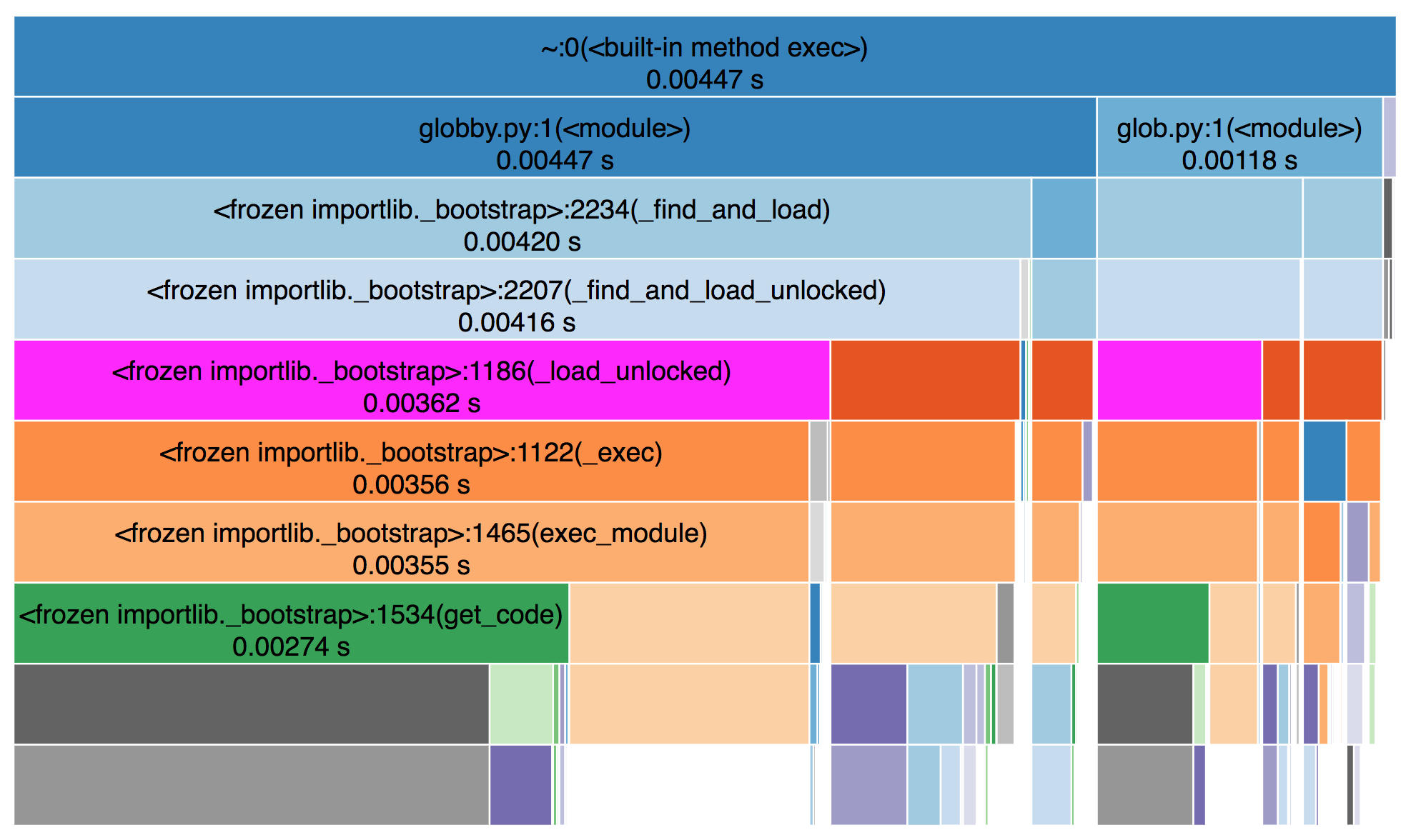
From the snakeviz docs, these charts show
the fraction of time spent in a function is represented by the extent of a visualization element, either the width of a rectangle or the angular extent of an arc.
I prefer the “sunburst” / angular extent style, but either works.
In this case, I noticed that ~95% of the time was being spent in
pandas._libs.lib.memory_usage_of_object, and most of that time was spent in
PandasArray.__getitem__ in pandas 1.0.3. This is where a bit of
pandas-specific knowledge comes in, but suffice to say, it looks fishy1.
As an aside, to create and share these snakeviz profiles, I ran the output of
the %snakeviz command through
svstatic and
uploaded that as a gist (using gist). I
then pasted the “raw” URL to https://rawgit.org/ to get the URL embedded here as
an iframe.
Line Profiling
With snakeviz, we’ve identified a function or two that’s slowing things down. If
I need more details on why that’s function is slow, I’ll use
line-profiler. In our example, we’ve
identified a couple of functions, IndexOpsMixin.memory_usage and
PandasArray.__getitem__ that could be inspected in detail.
You point line-profiler at one or more functions with -f and provide a
statement to execute. It will measure things about each line in the function,
including the number of times it’s hit and how long is spent on that line (per
hit and total)
In  [9]: %load_ext line_profiler
In [10]: %lprun -f pd.core.base.IndexOpsMixin.memory_usage df.memory_usage(deep=True)
Total time: 0.034319 s
File: /Users/taugspurger/miniconda3/envs/pandas=1.0.1/lib/python3.8/site-packages/pandas/core/base.py
Function: memory_usage at line 1340

Line #      Hits         Time  Per Hit   % Time  Line Contents
==============================================================
  1340                                               def memory_usage(self, deep=False):
  ...
  1363         1         56.0     56.0      0.2          if hasattr(self.array, "memory_usage"):
  1364                                                       return self.array.memory_usage(deep=deep)
  1365
  1366         1         11.0     11.0      0.0          v = self.array.nbytes
  1367         1         18.0     18.0      0.1          if deep and is_object_dtype(self) and not PYPY:
  1368         1      34233.0  34233.0     99.7              v += lib.memory_usage_of_objects(self.array)
  1369         1          1.0      1.0      0.0          return v
THe % time column clearly points to lib.memory_usage_of_objects. This is a
Cython function, so we can’t use line-profiler on it. But we know from the
snakeviz output above that we eventually get to PandasArray.__getitem__
In [11]: %lprun -f pd.arrays.PandasArray.__getitem__ df.memory_usage(deep=True)
Timer unit: 1e-06 s

Total time: 0.041508 s
File: /Users/taugspurger/miniconda3/envs/pandas=1.0.1/lib/python3.8/site-packages/pandas/core/arrays/numpy_.py
Function: __getitem__ at line 232

Line #      Hits         Time  Per Hit   % Time  Line Contents
==============================================================
   232                                               def __getitem__(self, item):
   233     10000       4246.0      0.4     10.2          if isinstance(item, type(self)):
   234                                                       item = item._ndarray
   235
   236     10000      25475.0      2.5     61.4          item = check_array_indexer(self, item)
   237
   238     10000       4394.0      0.4     10.6          result = self._ndarray[item]
   239     10000       4386.0      0.4     10.6          if not lib.is_scalar(item):
   240                                                       result = type(self)(result)
   241     10000       3007.0      0.3      7.2          return result
In this particular example, the most notable thing is that fact that we’re
calling this function 10,000 times, which amounts to once per item on our 10,000
row DataFrame. Again, the details of this specific example and the fix aren’t
too important, but the solution was to just stop doing that2.
The fix was provided by
@neilkg soon after the issue was identified, and
crucially included a new asv benchmark for memory_usage with object dtypes.
Hopefully we won’t regress on this again in the future.
Workflow issues
This setup is certainly better than nothing. But there are a few notable problems, some general and some specific to pandas:
Writing benchmarks is hard work (just like tests). There’s the general issue of writing and maintaining code. And on top of that, writing a good ASV benchmark requires some knowledge specific to ASV. And again, just like tests, your benchmarks can be trusted only as far as their coverage. For a large codebase like pandas you’ll need a decently large benchmark suite.
But that large benchmark suite comes with it’s own costs. Currently pandas’ full suite takes about 2 hours to run. This rules out running the benchmarks on most public CI providers. And even if we could finish it in time, we couldn’t really trust the results. These benchmarks, at least as written, really do need dedicated hardware to be stable over time. Pandas has a machine in my basement, but maintaining that has been a time-consuming, challenging process.

This is my current setup, which stuffs the benchmark server (the black Intel NUC) and a router next to my wife’s art storage. We reached this solution after my 2 year old unplugged the old setup (on my office floor) one too many times. Apologies for the poor cabling.
We deploy the benchmarks (for pandas
and a few other NumFOCUS projects) using Ansible. The scripts get the benchmarks
in place, Airflow to run them nightly, and supervisord to kick everything off.
The outputs are rsynced over to the pandas webserver and served at
https://pandas.pydata.org/speed/. You can
see pandas’ at
https://pandas.pydata.org/speed/pandas/.
If this seems like a house of cards waiting to tumble, that’s because it is.

Pandas has applied for a NumFOCUS small development grant to improve our
benchmark process. Ideally maintainers would be able to ask a bot @asv-bot run -b memory_usage which would kick off a process that pulled down the pull
request and ran the requested benchmarks on a dedicated machine (that isn’t
easily accessible by my children).
Recap
To summarize:
- We need benchmarks to monitor performance, especially over time
- We use tools like
asvto organize and benchmark continuously - When regressions occur, we use
snakevizandline-profilerto diagnose the problem
-
PandasArray is a very simple wrapper that implements pandas' ExtensionArray interface for 1d NumPy ndarrays, so it’s essentially just an ndarray. But, crucially, it’s a Python class so it’s getitem is relatively slow compared to numpy.ndarray’s getitem. ↩︎
-
It still does an elementwise getitem, but NumPy’s
__getitem__is much faster thanPandasArray’s. ↩︎
Compatibility Code
Most libraries with dependencies will want to support multiple versions of that dependency. But supporting old version is a pain: it requires compatibility code, code that is around solely to get the same output from versions of a library. This post gives some advice on writing compatibility code.
- Don’t write your own version parser
- Centralize all version parsing
- Use consistent version comparisons
- Use Python’s argument unpacking
- Clean up unused compatibility code
1. Don’t write your own version parser
It can be tempting just do something like
if pandas.__version__.split(".")[1] >= "25":
    ...
But that’s probably going to break, sometimes in unexpected ways. Use either distutils.version.LooseVersion
or packaging.version.parse which handles all the edge cases.
PANDAS_VERSION = LooseVersion(pandas.__version__)
2. Centralize all version parsing in a _compat.py file
The first section of compatibility code is typically a version check. It can be tempting to do the version-check inline with the compatibility code
if LooseVersion(pandas.__version__) >= "0.25.0":
    return pandas.concat(args, sort=False)
else:
    return pandas.concat(args)
Rather than that, I recommend centralizing the version checks in a central _compat.py file
that defines constants for each library version you need compatibility code for.
# library/_compat.py
import pandas


PANDAS_VERSION = LooseVersion(pandas.__version__)
PANDAS_0240 = PANDAS_VERSION >= "0.24.0
PANDAS_0250 = PANDAS_VERSION >= "0.25.0
This, combined with item 3, will make it easier to clean up your code (see below).
3. Use consistent version comparisons
Notice that I defined constants for each pandas version, PANDAS_0240,
PANDAS_0250. Those mean “the installed version of pandas is at least this
version”, since I used the >= comparison. You could instead define constants
like
PANDAS_LT_0240 = PANDAS_VERSION < "0.24.0"
That works too, just ensure that you’re consistent.
4. Use Python’s argument unpacking
Python’s argument unpacking helps avoid code duplication when the signature of a function changes.
    param_grid = {"estimator__alpha": [0.1, 10]}
    if SK_022:
        kwargs = {}
    else:
        kwargs = {"iid": False}
    gs = sklearn.model_selection.GridSearchCV(clf, param_grid, cv=3, **kwargs)
Using *args, and **kwargs to pass through version-dependent arguments lets you
have just a single call to the callable when the only difference is the
arguments passed.
5. Clean up unused compatibility code
Actively developed libraries may eventually drop support for old versions of dependency libraries. At a minimum, this involves removing the old version from your test matrix and bumping your required version in your dependency list. But ideally you would also clean up the now-unused compatibility code. The strategies laid out here intend to make that as easy as possible.
Consider the following.
# library/core.py
import pandas
from ._comapt import PANDAS_0250


def f(args):
    ...

    if PANDAS_0250:
        return pandas.concat(args, sort=False)
    else:
        return pandas.concat(args)
Now suppose it’s the future and we want to drop support for pandas older than 0.25.x
Now all the conditions checking if PANDAS_0250 are automatically true, so we’d
- Delete
PANDAS_0250from_compat.py - Remove the import in
core.py - Remove the
if PANDAS_0250check, and always have the True part of that condition
# library/core.py
import pandas

def f(args):
    ...
    return pandas.concat(args, sort=False)
I acknowledge that indirection can harm readability. In this case I think it’s warranted for actively maintained projects. Using inline version checks, perhaps with inconsistent comparisons, will make it harder to know when code is now unused. When integrated over the lifetime of the project, I find the strategies laid out here more readable.
]]>Dask Summit Recap
Last week was the first Dask Developer Workshop. This brought together many of the core Dask developers and its heavy users to discuss the project. I want to share some of the experience with those who weren’t able to attend.
This was a great event. Aside from any technical discussions, it was ncie to meet all the people. From new acquaintences to people you’re on weekly calls with, it was great to interact with everyone.
The workshop
During our brief introductions, everyone included a one-phrase description of what they’d most-like to see improved in the project. These can roughly be grouped as
- Project health: more maintainers, more maintainer diversity, more commercial adoption
- Deployments: Support for heterogeneous clusters (e.g. some workers with different resources) on more cluster managers. Easier deployments for various use cases (single user vs. small team of scientists vs. enterprise IT managing things for a large team)
- Documentation: Including example
- Data Access: Loading data from various sources
- Reliability: Especially on adaptive clusters, as workers come and go.
- Features: Including things like approximate nearest neighbors, shared clients between futures, multi-column sorting, MultiIndex for dask.dataframe
One of the themes of the workshop was requests for honest, critical feedback about what needs to improve. Overall, people had great things to say about Dask and the various sub-projects but there’s always things to improve.
Dask sits at a pretty interesting place in the scientific Python ecosystem. It (and its users) are power-users of many libraries. It acts as a nice coordination point for many projects. We had maintainers from projects like NumPy, pandas, scikit-learn, Apache Arrow, cuDF, and others.
]]>This post describes the start of a journey to get pandas’ documentation running on Binder. The end result is this nice button:
![]()
For a while now I’ve been jealous of Dask’s examples repository. That’s a repository containing a collection of Jupyter notebooks demonstrating Dask in action. It stitches together some tools to present a set of documentation that is both viewable as a static site at examples.dask.org, and as a executable notebooks on mybinder.
A bit of background on binder: it’s a tool for creating a shareable computing environment. This is perfect for introductory documentation. A prospective user may want to just try out a library to get a feel for it before they commit to installing. BinderHub is a tool for deploying binder services. You point a binderhub deployment (like mybinder) at a git repository with a collection of notebooks and an environment specification, and out comes your executable documentation.
Thanks to a lot of hard work by contributors and maintainers, the code examples in pandas’ documentation are already runnable (and this is verified on each commit). We use the IPython Sphinx Extension to execute examples and include their output. We write documentation like
.. ipython:: python

   import pandas as pd
   s = pd.Series([1, 2])
   s
Which is then executed and rendered in the HTML docs as
In [1]: import pandas as pd

In [2]: s = pd.Series([1, 2, 3])

In [3]: s
Out[3]:
0    1
1    2
2    3
dtype: int64
So we have the most important thing: a rich source of documentation that’s already runnable.
There were a couple barriers to just pointing binder at
https://github.com/pandas-dev/pandas, however. First, binder builds on top of
a tool called repo2docker. This
is what takes your Git repository and turns it into a Docker image that users
will be dropped into. When someone visits the URL, binder will first check to
see if it’s built a docker image. If it’s already cached, then that will just be
loaded. If not, binder will have to clone the repository and build it from
scratch, a time-consuming process. Pandas receives 5-10 commits per day, meaning
many users would visit the site and be stuck waiting for a 5-10 minute docker
build.1
Second, pandas uses Sphinx and ReST for its documentation. Binder needs a collection
of Notebooks. Fortunately, the fine folks at QuantEcon
(a fellow NumFOCUS project) wrote
sphinxcontrib-jupyter, a tool
for turning ReST files to Jupyter notebooks. Just what we needed.
So we had some great documentation that already runs, and a tool for converting ReST files to Jupyter notebooks. All the pieces were falling into place!
Unfortunately, my first attempt failed. sphinxcontrib-jupyter looks for directives
like
.. code:: python
while pandas uses
.. ipython:: python
I started slogging down a path to teach sphinxcontrib-jupyter how to recognize
the IPython directive pandas uses when my kid woke up from his nap. Feeling
dejected I gave up.
But later in the day, I had the (obvious in hindsight) realization that we have
plenty of tools for substituting lines of text. A few (non-obvious) lines of
bash
later
and we were ready to go. All the .. ipython:: python directives were now .. code:: python. Moral of the story: take breaks.
My work currently lives in this repository, and the notebooks are runnable on mybinder. But the short version is
- We include github.com/pandas-dev/pandas as a submodule (which repo2docker supports just fine)
- We patch pandas Sphinx config to include sphinxcontrib-jupyter and its configuration
- We patch pandas source docs to change the ipython directives to be
.. code:: pythondirectives.
I’m reasonably happy with how things are shaping up. I plan to migrate my repository to the pandas organization and propose a few changes to the pandas documentation (like a small header pointing from the rendered HTML docs to the binder). If you’d like to follow along, subscribe to this pandas issue.
I’m also hopeful that other projects can apply a similar approach to their documentation too.
-
I realize now that binder can target a specific branch or commit. I’m not sure if additional commits to that repository will trigger a rebuild, but I suspect not. We still needed to solve problem 2 though. ↩︎
This post describes a few protocols taking shape in the scientific Python community. On their own, each is powerful. Together, I think they enable for an explosion of creativity in the community.
Each of the protocols / interfaces we’ll consider deal with extending.
- NEP-13: NumPy
__array_ufunc__ - NEP-18: NumPy
__array_function__ - Pandas Extension types
- Custom Dask Collections
First, a bit of brief background on each.
NEP-13 and NEP-18, each deal with using the NumPy API on non-NumPy ndarray
objects. For example, you might want to apply a ufunc like np.log to a Dask
array.
>>> a = da.random.random((10, 10))
>>> np.log(a)
dask.array<log, shape=(10, 10), dtype=float64, chunksize=(10, 10)>
Prior to NEP-13, dask.array needed it’s own namespace of ufuncs like da.log,
since np.log would convert the Dask array to an in-memory NumPy array
(probably blowing up your machine’s memory). With __array_ufunc__ library
authors and users can all just use NumPy ufuncs, without worrying about the type of
the Array object.
While NEP-13 is limited to ufuncs, NEP-18 applies the same idea to most of the
NumPy API. With NEP-18, libraries written to deal with NumPy ndarrays may
suddenly support any object implementing __array_function__.
I highly recommend reading this blog
post for more on the motivation
for __array_function__. Ralph Gommers gave a nice talk on the current state of
things at PyData Amsterdam 2019, though this is
an active area of development.
Pandas added extension types to allow third-party libraries to solve domain-specific problems in a way that gels nicely with the rest of pandas. For example, cyberpandas handles network data, while geopandas handles geographic data. When both implement extension arrays it’s possible to operate on a dataset with a mixture of geographic and network data in the same DataFrame.
Finally, Dask defines a Collections Interface so that any object can be a first-class citizen within Dask. This is what ensures XArray’s DataArray and Dataset objects work well with Dask.
Series.__array_ufunc__
Now, onto the fun stuff: combining these interfaces across objects and
libraries. https://github.com/pandas-dev/pandas/pull/23293 is a pull request
adding Series.__array_ufunc__. There are a few subtleties, but the basic idea
is that a ufunc applied to a Series should
- Unbox the array (ndarray or extension array) from the Series
- Apply the ufunc to the Series (honoring the array’s
__array_ufunc__if needed) - Rebox the output in a Series (with the original index and name)
For example, pandas’ SparseArray implements __array_ufunc__. It works by
calling the ufunc twice, once on the sparse values (e.g. the non-zero values),
and once on the scalar fill_value. The result is a new SparseArray with the
same memory usage. With that PR, we achieve the same thing when operating on a
Series containing an ExtensionArray.
>>> ser = pd.Series(pd.SparseArray([-10, 0, 10] + [0] * 100000))
>>> ser
0        -10
1          0
2         10
3          0
4          0
          ..
99998      0
99999      0
100000     0
100001     0
100002     0
Length: 100003, dtype: Sparse[int64, 0]

>>> n [20]: np.sign(ser)
0        -1
1         0
2         1
3         0
4         0
         ..
99998     0
99999     0
100000    0
100001    0
100002    0
Length: 100003, dtype: Sparse[int64, 0]
Previously, that would have converted the SparseArray to a dense NumPy
array, blowing up your memory, slowing things down, and giving the incorrect result.
IPArray.__array_function__
To demonstrate __array_function__, we’ll implement it on IPArray.
    def __array_function__(self, func, types, args, kwargs):
        cls = type(self)
        if not all(issubclass(t, cls) for t in types):
            return NotImplemented
        return HANDLED_FUNCTIONS[func](*args, **kwargs)
IPArray is pretty domain-specific, so we place ourself down at the bottom
priority by returning NotImplemented if there are any types we don’t recognize
(we might consider handling Python’s stdlib ipaddres.IPv4Address and
ipaddres.IPv6Address objects too).
And then we start implementing the interface. For example, concatenate.
@implements(np.concatenate)
def concatenate(arrays, axis=0, out=None):
    if axis != 0:
        raise NotImplementedError(f"Axis != 0 is not supported. (Got {axis}).")
    return IPArray(np.concatenate([array.data for array in arrays]))
With this, we can successfully concatenate two IPArrays
>>> a = cyberpandas.ip_range(4)
>>> b = cyberpandas.ip_range(10, 14)
>>> np.concatenate([a, b])
IPArray(['0.0.0.0', '0.0.0.1', '0.0.0.2', '0.0.0.3', '0.0.0.10', '0.0.0.11', '0.0.0.12', '0.0.0.13'])
Extending Dask
Finally, we may wish to make IPArray work well with dask.dataframe, to do
normal cyberpandas operations in parallel, possibly distributed on a cluster.
This requires a few changes:
- Updating
IPArrayto work on either NumPy or Dask arrays - Implementing the Dask Collections interface on
IPArray. - Registering an
ipaccessor withdask.dataframe, just like withpandas.
This is demonstrated in https://github.com/ContinuumIO/cyberpandas/pull/39
In [28]: ddf
Out[28]:
Dask DataFrame Structure:
                 A
npartitions=2
0               ip
6              ...
11             ...
Dask Name: from_pandas, 2 tasks

In [29]: ddf.A.ip.netmask()
Out[29]:
Dask Series Structure:
npartitions=2
0      ip
6     ...
11    ...
Name: A, dtype: ip
Dask Name: from-delayed, 22 tasks

In [30]: ddf.A.ip.netmask().compute()
Out[30]:
0     255.255.255.255
1     255.255.255.255
2     255.255.255.255
3     255.255.255.255
4     255.255.255.255
5     255.255.255.255
6     255.255.255.255
7     255.255.255.255
8     255.255.255.255
9     255.255.255.255
10    255.255.255.255
11    255.255.255.255
dtype: ip
Conclusion
I think that these points of extension.
]]>Scikit-Learn 0.20.0 will contain some nice new features for working with tabular data. This blogpost will introduce those improvements with a small demo. We’ll then see how Dask-ML was able to piggyback on the work done by scikit-learn to offer a version that works well with Dask Arrays and DataFrames.
import dask
import dask.array as da
import dask.dataframe as dd
import numpy as np
import pandas as pd
import seaborn as sns
import fastparquet
from distributed import Client
from distributed.utils import format_bytes
Background
For the most part, Scikit-Learn uses NumPy ndarrays or SciPy sparse matricies for its in-memory data structures. This is great for many reasons, but one major drawback is that you can’t store heterogenous (AKA tabular) data in these containers. These are datasets where different columns of the table have different data types (some ints, some floats, some strings, etc.).
Pandas was built to work with tabular data.
Scikit-Learn was built to work with NumPy ndarrays and SciPy sparse matricies.
So there’s some friction when you use the two together.
Perhaps someday things will be perfectly smooth, but it’s a challenging problem that will require work from several communities to fix.
In this PyData Chicago talk, I discuss the differences between the two data models of scikit-learn and pandas, and some ways of working through it. The second half of the talk is mostly irrelevant now that ColumnTransformer is in scikit-learn.
ColumnTransformer in Scikit-Learn
At SciPy 2018, Joris Van den Bossche (a scikit-learn and pandas core developer) gives an update on some recent improvements to scikit-learn to make using pandas and scikit-learn together better.
The biggest addition is sklearn.compose.ColumnTransformer, a transformer for working with tabular data.
The basic idea is to specify pairs of (column_selection, transformer). The transformer will be applied just to the selected columns, and the remaining columns can be passed through or dropped. Column selections can be integer positions (for arrays), names (for DataFrames) or a callable.
Here’s a small example on the “tips” dataset.
df = sns.load_dataset('tips')
df.head()
| total_bill | tip | sex | smoker | day | time | size | |
|---|---|---|---|---|---|---|---|
| 0 | 16.99 | 1.01 | Female | No | Sun | Dinner | 2 |
| 1 | 10.34 | 1.66 | Male | No | Sun | Dinner | 3 |
| 2 | 21.01 | 3.50 | Male | No | Sun | Dinner | 3 |
| 3 | 23.68 | 3.31 | Male | No | Sun | Dinner | 2 |
| 4 | 24.59 | 3.61 | Female | No | Sun | Dinner | 4 |
Our target is whether the tip was larger than 15%.
X = df.drop("tip", axis='columns')
y = df.tip / df.total_bill > 0.15
We’ll make a small pipeline that one-hot encodes the categorical columns (sex, smoker, day, time) before fitting a random forest. The numeric columns (total_bill, size) will be passed through as-is.
import sklearn.compose
import sklearn.ensemble
import sklearn.pipeline
import sklearn.preprocessing
We use make_column_transformer to create the ColumnTransformer.
categorical_columns = ['sex', 'smoker', 'day', 'time']
categorical_encoder = sklearn.preprocessing.OneHotEncoder(sparse=False)

transformers = sklearn.compose.make_column_transformer(
    (categorical_columns, categorical_encoder),
    remainder='passthrough'
)
This is just a regular scikit-learn estimator, which can be placed in a pipeline.
pipe = sklearn.pipeline.make_pipeline(
    transformers,
    sklearn.ensemble.RandomForestClassifier(n_estimators=100)
)

pipe.fit(X, y)
pipe.score(X, y)
1.0
We’ve likely overfitted, but that’s not really the point of this article. We’re more interested in the pre-processing side of things.
ColumnTransformer in Dask-ML
ColumnTransfomrer was added to Dask-ML in https://github.com/dask/dask-ml/pull/315.
Ideally, we wouldn’t need that PR at all. We would prefer for dask’s collections (and pandas dataframes) to just be handled gracefully by scikit-learn. The main blocking issue is that the Python community doesn’t currently have a way to write “concatenate this list of array-like objects together” in a generic way. That’s being worked on in NEP-18.
So for now, if you want to use ColumnTransformer with dask objects, you’ll have to use dask_ml.compose.ColumnTransformer, otherwise your large Dask Array or DataFrame would be converted to an in-memory NumPy array.
As a footnote to this section, the initial PR in Dask-ML was much longer.
I only needed to override one thing (the function _hstack used to glue the results back together). But that was being called from several places, and so I had to override all those places as well. I was able to work with the scikit-learn developers to make _hstack a staticmethod on ColumnTranformer, so any library wishing to extend ColumnTransformer can do so more easily now. The Dask project values working with the existing community.
Challenges with Scaling
Many strategies for dealing with large datasets rely on processing the data in chunks.
That’s the basic idea behind Dask DataFrame: a Dask DataFrame consists of many pandas DataFrames.
When you write ddf.column.value_counts(), Dask builds a task graph with many pandas.value_counts, and a final aggregation step so that you end up with the same end result.
But chunking can cause issues when there are variations in your dataset and the operation you’re applying depends on the data. For example, consider scikit-learn’s OneHotEncoder. By default, it looks at the data and creates a column for each unique value.
enc = sklearn.preprocessing.OneHotEncoder(sparse=False)
enc.fit_transform([['a'], ['a'], ['b'], ['c']])
array([[1., 0., 0.],
       [1., 0., 0.],
       [0., 1., 0.],
       [0., 0., 1.]])
But let’s suppose we wanted to process that in chunks of two, first [['a'], ['a']], then [['b'], ['c']].
enc.fit_transform([['a'], ['a']])
array([[1.],
       [1.]])
enc.fit_transform([['b'], ['c']])
array([[1., 0.],
       [0., 1.]])
We have a problem! Two in fact:
- The shapes don’t match. The first batch only saw “a”, so the output shape is
(2, 1). We can’t concatenate these results vertically - The meaning of the first column of the output has changed. In the first batch, the first column meant “a” was present. In the second batch, it meant “b” was present.
If we happened to know the set of possible values ahead of time, we could pass those to CategoricalEncoder. But storing that set of possible values separate from the data is fragile. It’d be better to store the possible values in the data type itself.
That’s exactly what pandas Categorical does. We can confidently know the number of columns in the categorical-encoded data by just looking at the type. Because this is so important in a distributed dataset context, dask_ml.preprocessing.OneHotEncoder differs from scikit-learn when passed categorical data: we use pandas’ categorical information.
A larger Example
We’ll work with the Criteo dataset. This has a mixture of numeric and categorical features. It’s also a large dataset, which presents some challenges for many pre-processing methods.
The full dataset is from http://labs.criteo.com/2013/12/download-terabyte-click-logs/. We’ll work with a sample.
client = Client()
ordinal_columns = [
    'category_0', 'category_1', 'category_2', 'category_3',
    'category_4', 'category_6', 'category_7', 'category_9',
    'category_10', 'category_11', 'category_13', 'category_14',
    'category_17', 'category_19', 'category_20', 'category_21',
    'category_22', 'category_23',
]

onehot_columns = [
    'category_5', 'category_8', 'category_12',
    'category_15', 'category_16', 'category_18',
    'category_24', 'category_25',
]

numeric_columns = [f'numeric_{i}' for i in range(13)]
columns = ['click'] + numeric_columns + onehot_columns + ordinal_columns
The raw data is a single large CSV. That’s been split with this script and I took a 10% sample with this script, which was written to a directory of parquet files. That’s what we’ll work with.
sample = dd.read_parquet("data/sample-10.parquet/")

# Convert unknown categorical to known.
# See note later on.

pf = fastparquet.ParquetFile("data/sample-10.parquet/part.0.parquet")
cats = pf.grab_cats(onehot_columns)

sample = sample.assign(**{
    col: sample[col].cat.set_categories(cats[col]) for col in onehot_columns
})
Our goal is to predict ‘click’ using the other columns.
y = sample['click']
X = sample.drop("click", axis='columns')
Now, let’s lay out our pre-processing pipeline. We have three types of columns
- Numeric columns
- Low-cardinality categorical columns
- High-cardinality categorical columns
Each of those will be processed differently.
- Numeric columns will have missing values filled with the column average and standard scaled
- Low-cardinality categorical columns will be one-hot encoded
- High-cardinality categorical columns will be deterministically hashed and standard scaled
You’ll probably want to quibble with some of these choices, but right now, I’m just interested in the ability to do these kinds of transformations at all.
We need to define a couple custom estimators, one for hashing the values of a dask dataframe, and one for converting a dask dataframe to a dask array.
import sklearn.base

def hash_block(x: pd.DataFrame) -> pd.DataFrame:
    """Hash the values in a DataFrame."""
    hashed = [
        pd.Series(pd.util.hash_array(data.values), index=x.index, name=col)
        for col, data in x.iteritems()
    ]
    return pd.concat(hashed, axis='columns')


class HashingEncoder(sklearn.base.BaseEstimator, sklearn.base.TransformerMixin):
    def fit(self, X, y=None):
        return self

    def transform(self, X, y=None):
        if isinstance(X, pd.DataFrame):
            return hash_block(X)
        elif isinstance(X, dd.DataFrame):
            return X.map_partitions(hash_block)
        else:
            raise ValueError("Unexpected type '{}' for 'X'".format(type(X)))


class ArrayConverter(sklearn.base.BaseEstimator, sklearn.base.TransformerMixin):
    """Convert a Dask DataFrame to a Dask Array with known lengths"""
    def __init__(self, lengths=None):
        self.lengths = lengths

    def fit(self, X, y=None):
        return self

    def transform(self, X, y=None):
        return X.to_dask_array(lengths=self.lengths)
For the final stage, Dask-ML needs to have a Dask Array with known chunk lengths. So let’s compute those ahead of time, and get a bit of info about how large the dataset is while we’re at it.
lengths = sample['click'].map_partitions(len)
nbytes = sample.memory_usage(deep=True).sum()

lengths, nbytes = dask.compute(lengths, nbytes)
lengths = tuple(lengths)

format_bytes(nbytes)
'19.20 GB'
We we’ll be working with about 20GB of data on a laptop with 16GB of RAM. We’ll clearly be relying on Dask to do the operations in parallel, while keeping things in a small memory footprint.
from dask_ml.compose import make_column_transformer
from dask_ml.preprocessing import StandardScaler, OneHotEncoder
from dask_ml.wrappers import Incremental
from dask_ml.impute import SimpleImputer

from sklearn.pipeline import make_pipeline
from sklearn.preprocessing import FunctionTransformer
from sklearn.linear_model import SGDClassifier
Now for the pipeline.
onehot_encoder = OneHotEncoder(sparse=False)
hashing_encoder = HashingEncoder()
nan_imputer = SimpleImputer()

to_numeric = make_column_transformer(
    (onehot_columns, onehot_encoder),
    (ordinal_columns, hashing_encoder),
    remainder='passthrough',
)

fill_na = make_column_transformer(
    (numeric_columns, nan_imputer),
    remainder='passthrough'
)

scaler = make_column_transformer(
    (list(numeric_columns) + list(ordinal_columns), StandardScaler()),
    remainder='passthrough'
)


clf = Incremental(
    SGDClassifier(loss='log',
                  random_state=0,
                  max_iter=1000)
)

pipe = make_pipeline(to_numeric, fill_na, scaler, ArrayConverter(lengths=lengths), clf)
pipe
Pipeline(memory=None,
     steps=[('columntransformer-1', ColumnTransformer(n_jobs=1, preserve_dataframe=True, remainder='passthrough',
         sparse_threshold=0.3, transformer_weights=None,
         transformers=[('onehotencoder', OneHotEncoder(categorical_features=None, categories='auto',
       dtype=<class 'numpy.float6...ion=0.1, verbose=0, warm_start=False),
      random_state=None, scoring=None, shuffle_blocks=True))])
Overall it reads pretty similarly to how we described it in prose. We specify
- Onehot the low-cardinality categoricals, hash the others
- Fill missing values in the numeric columns
- Standard scale the numeric and hashed columns
- Fit the incremental SGD
And again, these ColumnTransformers are just estimators so we stick them in a regular scikit-learn Pipeline before calling .fit:
%%time pipe.fit(X, y.to_dask_array(lengths=lengths), incremental__classes=[0, 1])
CPU times: user 7min 7s, sys: 41.6 s, total: 7min 48s Wall time: 16min 42sPipeline(memory=None, steps=[(‘columntransformer-1’, ColumnTransformer(n_jobs=1, preserve_dataframe=True, remainder=‘passthrough’, sparse_threshold=0.3, transformer_weights=None, transformers=[(‘onehotencoder’, OneHotEncoder(categorical_features=None, categories=‘auto’, dtype=<class ’numpy.float6…ion=0.1, verbose=0, warm_start=False), random_state=None, scoring=None, shuffle_blocks=True))])
Discussion
Some aspects of this workflow could be improved.
-
Dask, fastparquet, pyarrow, and pandas don’t currently have a way to specify the categorical dtype of a column split across many files. Each file (parition) is treated independently. This results in categorials with unknown categories in the Dask DataFrame. Since we know that the categories are all the same, we’re able to read in the first files categories and assign those to the entire DataFrame. But this is a bit fragile, as it relies on an assumption not necessarily guaranteed by the file structure.
-
There’s of IO. As written, each stage of the pipeline that has to see the data does a full read of the dataset. We end up reading the entire dataset something like 5 times. https://github.com/dask/dask-ml/issues/192 has some discussion on ways we can progress through a pipeline. If your pipeline consists entirely of estimators that learn incrementally, it may make sense to send each block of data through the entire pipeline, rather than sending all the data to the first step, then all the data to the second, and so on. I’ll note, however, that you can avoid the redundant IO by loading your data into distributed RAM on a Dask cluster. But I was just trying things out on my laptop.
Still, it’s worth noting that we’ve successfully fit a reasonably complex pipeline on a larger-than-RAM dataset using our laptop. That’s something!
ColumnTransformer will be available in scikit-learn 0.20.0. This also contains the changes for distributed joblib I blogged about earlier. The first release candidate is available now.
For more, visit the Dask, Dask-ML, and scikit-learn documentation.
]]>This work is supported by Anaconda Inc.
This post describes a recent improvement made to TPOT. TPOT is an automated machine learning library for Python. It does some feature engineering and hyper-parameter optimization for you. TPOT uses genetic algorithms to evaluate which models are performing well and how to choose new models to try out in the next generation.
Parallelizing TPOT
In TPOT-730, we made some modifications to TPOT to support distributed training. As a TPOT user, the only changes you need to make to your code are
- Connect a client to your Dask Cluster
- Specify the
use_dask=Trueargument to your TPOT estimator
From there, all the training will use your cluster of machines. This screencast shows an example on an 80-core Dask cluster.
Commentary
Fitting a TPOT estimator consists of several stages. The bulk of the time is
spent evaluating individual scikit-learn pipelines. Dask-ML already had code for
splitting apart a scikit-learn Pipeline.fit call into individual tasks. This
is used in Dask-ML’s hyper-parameter optimization to avoid repeating
work. We were able to drop-in Dask-ML’s fit and scoring method
for the one already used in TPOT. That small change allows fitting the many
individual models in a generation to be done on a cluster.
There’s still some room for improvement. Internal to TPOT, some time is spent determining the next set of models to try out (this is the “mutation and crossover phase”). That’s not (yet) been parallelized with Dask, so you’ll notice some periods of inactivity on the cluster.
Next Steps
This will be available in the next release of TPOT. You can try out a small example now on the dask-examples binder.
Stepping back a bit, I think this is a good example of how libraries can use
Dask internally to parallelize workloads for their users. Deep down in TPOT
there was a single method for fitting many scikit-learn models on some data and
collecting the results. Dask-ML has code for building a task graph that does
the same thing. We were able to swap out the eager TPOT code for the lazy dask
version, and get things distributed on a cluster. Projects like xarray
have been able to do a similar thing with dask Arrays in place of NumPy
arrays. If Dask-ML hadn’t already had that code,
dask.delayed could have been used instead.
If you have a library that you think could take advantage of Dask, please reach out!
]]>The other day, I put up a Twitter poll asking a simple question: What’s the type of series.values?
Pop Quiz! What are the possible results for the following:
— Tom Augspurger (@TomAugspurger) August 6, 2018
>>> type(pandas.Series.values)
I was a bit limited for space, so I’ll expand on the options here. Choose as many as you want.
- NumPy ndarray
- pandas Categorical (or all of the above)
- An Index or any of it’s subclasses (DatetimeIndex, CategoricalIndex, RangeIndex, etc.) (or all of the above)
- None or all of the above
I was prompted to write this post because a.) this is an (unfortunately) confusing topic and b.) it’s undergoing a lot of change right now (and, c.) I had this awesome title in my head).
The Answer
Unfortunately I kind of messed up the poll. Things are even more complex than I initially thought.
As best I can tell, the possible types for series.values are
- NumPy ndarray
- pandas Categorical
- pandas SparseArray (I forgot about this one in the poll)
So going with the cop-out “best-available” answer, I would have said that 2 was the best answer in the poll. SparseArray is technically and ndarray subclass (for now), so technically 2 is correct, but that’s a few too many technicallys for me.
The Explanation
So, that’s a bit of a mess. How’d we get here? Or, stepping back a bit, what even is an array? What’s a dataframe?
NumPy arrays are N-dimensional and homogenous. Every element in the array has to have the same data type.
Pandas dataframes are 2-dimensional and heterogenous. Different columns can have different data types. But every element in a single column (Series) has the same data type. I like to think of DataFrames as containers for Series. Stepping down a dimension, I think of Series as containers for 1-D arrays. In an ideal world, we could say Series are containers for NumPy ararys, but that’s not quite the case.
While there’s a lot of overlap between the pandas and NumPy communites, there are still differences.
Pandas users place different value on different features, so pandas has restricted and extended NumPy’s type system in a few directions.
For example, early Pandas users (many of them in the financial sector) needed datetimes with timezones, but didn’t really care about lower-precision timestamps like datetime64[D].
So pandas limited its scope to just nanosecond-precision datetimes (datetime64[ns]) and extended it with some metedata for the timezone.
Likewise for Categorical, period, sparse, interval, etc.
So back to Series.values; pandas had a choice: should Series.values always be a NumPy array, even if it means losing information like the timezone or categories, and even if it’s slow or could exhaust your memory (large categorical or sparse arrays)?
Or should it faithfully represent the data, even if that means not returning an ndarray?
I don’t think there’s a clear answer to this question. Both options have their downsides.
In the end, we ended up with a messy compromise, where some things return ndarrays, some things return something else (Categorical), and some things do a bit of conversion before returning an ndarary.
For example, off the top of your head, do you know what the type of Series.values is for timezone-aware data?
In [2]: pd.Series(pd.date_range('2017', periods=4, tz='US/Eastern'))
Out[2]:
0   2017-01-01 00:00:00-05:00
1   2017-01-02 00:00:00-05:00
2   2017-01-03 00:00:00-05:00
3   2017-01-04 00:00:00-05:00
dtype: datetime64[ns, US/Eastern]

In [3]: pd.Series(pd.date_range('2017', periods=4, tz='US/Eastern')).values
Out[3]:
array(['2017-01-01T05:00:00.000000000', '2017-01-02T05:00:00.000000000',
       '2017-01-03T05:00:00.000000000', '2017-01-04T05:00:00.000000000'],
      dtype='datetime64[ns]')
With the wisdom of Solomon, we decided to have it both ways; the values are converted to UTC and the timezone is dropped. I don’t think anyone would claim this is ideal, but it was backwards compatibile-ish. Given the constraints, it wasn’t the worst choice in the world.
The Near Future
In pandas 0.24, we’ll (hopefully) have a good answer for what series.values is: a NumPy array or an ExtensionArray.
For regular data types represented by NumPy, you’ll get an ndarray.
For extension types (implemented in pandas or elsewhere) you’ll get an ExtensionArray.
If you’re using Series.values, you can rely on the set of methods common to each.
But that raises the question: why are you using .values in the first place?
There are some legitmate use cases (disabling automatic alignment, for example),
but for many things, passing a Series will hopefully work as well as a NumPy array.
To users of pandas, I recommend avoiding .values as much as possible.
If you know that you need an ndarray, you’re probably best of using np.asarray(series).
That will do the right thing for any data type.
The Far Future
I’m hopeful that some day all we’ll have a common language for these data types. There’s a lot going on in the numeric Python ecosystem right now. Stay tuned!
]]>This is part 1 in my series on writing modern idiomatic pandas.
As I sit down to write this, the third-most popular pandas question on StackOverflow covers how to use pandas for large datasets. This is in tension with the fact that a pandas DataFrame is an in memory container. You can’t have a DataFrame larger than your machine’s RAM. In practice, your available RAM should be several times the size of your dataset, as you or pandas will have to make intermediate copies as part of the analysis.
Historically, pandas users have scaled to larger datasets by switching away from pandas or using iteration. Both of these are perfectly valid approaches, but changing your workflow in response to scaling data is unfortunate. I use pandas because it’s a pleasant experience, and I would like that experience to scale to larger datasets. That’s what Dask, a parallel computing library, enables. We’ll discuss Dask in detail later. But first, let’s work through scaling a simple analysis to a larger than memory dataset.
Our task is to find the 100 most-common occupations reported in the FEC’s individual contributions dataest. The files are split by election cycle (2007-2008, 2009-2010, …). You can find some scripts for downloading the data in this repository. My laptop can read in each cycle’s file individually, but the full dataset is too large to read in at once. Let’s read in just 2010’s file, and do the “small data” version.
from pathlib import Path

import pandas as pd
import seaborn as sns

df = pd.read_parquet("data/indiv-10.parq", columns=['occupation'], engine='pyarrow')

most_common = df.occupation.value_counts().nlargest(100)
most_common
    RETIRED                    279775
    ATTORNEY                   166768
    PRESIDENT                   81336
    PHYSICIAN                   73015
    HOMEMAKER                   66057
                                ...
    C.E.O.                       1945
    EMERGENCY PHYSICIAN          1944
    BUSINESS EXECUTIVE           1924
    BUSINESS REPRESENTATIVE      1879
    GOVERNMENT AFFAIRS           1867
    Name: occupation, Length: 100, dtype: int64
After reading in the file, our actual analysis is a simple 1-liner using two operations built into pandas. Truly, the best of all possible worlds.
Next, we’ll do the analysis for the entire dataset, which is larger than memory, in two ways. First we’ll use just pandas and iteration. Then we’ll use Dask.
Using Iteration
To do this with just pandas we have to rewrite our code, taking care to never have too much data in RAM at once. We will
- Create a global
total_countsSeries that contains the counts from all of the files processed so far - Read in a file
- Compute a temporary variable
countswith the counts for just this file - Add that temporary
countsinto the globaltotal_counts - Select the 100 largest with
.nlargest
This works since the total_counts Series is relatively small, and each year’s data fits in RAM individually. Our peak memory usage should be the size of the largest individual cycle (2015-2016) plus the size of total_counts (which we can essentially ignore).
files = sorted(Path("data/").glob("indiv-*.parq"))

total_counts = pd.Series()

for year in files:
    df = pd.read_parquet(year, columns=['occupation'],
                         engine="pyarrow")
    counts = df.occupation.value_counts()
    total_counts = total_counts.add(counts, fill_value=0)

total_counts = total_counts.nlargest(100).sort_values(ascending=False)
RETIRED                    4769520
NOT EMPLOYED               2656988
ATTORNEY                   1340434
PHYSICIAN                   659082
HOMEMAKER                   494187
                            ...
CHIEF EXECUTIVE OFFICER      26551
SURGEON                      25521
EDITOR                       25457
OPERATOR                     25151
ORTHOPAEDIC SURGEON          24384
Name: occupation, Length: 100, dtype: int64
While this works, our small one-liner has ballooned in size (and complexity; should you really have to know about Series.add’s fill_value parameter for this simple analysis?). If only there was a better way…
Using Dask
With Dask, we essentially recover our original code. We’ll change our import to use dask.dataframe.read_parquet, which returns a Dask DataFrame.
import dask.dataframe as dd
df = dd.read_parquet("data/indiv-*.parquet", engine='pyarrow', columns=['occupation'])

most_common = df.occupation.value_counts().nlargest(100)
most_common.compute().sort_values(ascending=False)
RETIRED                    4769520
NOT EMPLOYED               2656988
ATTORNEY                   1340434
PHYSICIAN                   659082
HOMEMAKER                   494187
                            ...
CHIEF EXECUTIVE OFFICER      26551
SURGEON                      25521
EDITOR                       25457
OPERATOR                     25151
ORTHOPAEDIC SURGEON          24384
Name: occupation, Length: 100, dtype: int64
There are a couple differences from the original pandas version, which we’ll discuss next, but overall I hope you agree that the Dask version is nicer than the version using iteration.
Dask
Now that we’ve seen dask.dataframe in action, let’s step back and discuss Dask a bit. Dask is an open-source project that natively parallizes Python. I’m a happy user of and contributor to Dask.
At a high-level, Dask provides familiar APIs for large N-dimensional arrays, large DataFrames, and familiar ways to parallelize custom algorithms.
At a low-level, each of these is built on high-performance task scheduling that executes operations in parallel. The low-level details aren’t too important; all we care about is that
- Dask works with task graphs (tasks: functions to call on data, and graphs: the relationships between tasks).
- This is a flexible and performant way to parallelize many different kinds of problems.
To understand point 1, let’s examine the difference between a Dask DataFrame and a pandas DataFrame. When we read in df with dd.read_parquet, we received a Dask DataFrame.
df
| occupation | |
|---|---|
| npartitions=35 | |
| object | |
| ... | |
| ... | ... |
| ... | |
| ... |
A Dask DataFrame consists of many pandas DataFrames arranged by the index. Dask is really just coordinating these pandas DataFrames.

All the actual computation (reading from disk, computing the value counts, etc.) eventually use pandas internally. If I do df.occupation.str.len, Dask will coordinate calling pandas.Series.str.len on each of the pandas DataFrames.
Those reading carefully will notice a problem with the statement “A Dask DataFrame consists of many pandas DataFrames”. Our initial problem was that we didn’t have enough memory for those DataFrames! How can Dask be coordinating DataFrames if there isn’t enough memory? This brings us to the second major difference: Dask DataFrames (and arrays) are lazy. Operations on them don’t execute and produce the final result immediately. Rather, calling methods on them builds up a task graph.
We can visualize task graphs using graphviz. For the blog, I’ve trimmed down the example to be a subset of the entire graph.
df.visualize(rankdir='LR')

df (the dask DataFrame consisting of many pandas DataFrames) has a task graph with 5 calls to a parquet reader (one for each file), each of which produces a DataFrame when called.
Calling additional methods on df adds additional tasks to this graph. For example, our most_common Series has three additional calls
- Select the
occupationcolumn (__getitem__) - Perform the value counts
- Select the 100 largest values
most_common = df.occupation.value_counts().nlargest(100)
most_common
    Dask Series Structure:
    npartitions=1
        int64
          ...
    Name: occupation, dtype: int64
    Dask Name: series-nlargest-agg, 113 tasks
Which we can visualize.
most_common.visualize(rankdir='LR')

So most_common doesn’t hold the actual answer yet. Instead, it holds a recipe for the answer; a list of all the steps to take to get the concrete result. One way to ask for the result is with the compute method.
most_common.compute()
    RETIRED                    4769520
    NOT EMPLOYED               2656988
    ATTORNEY                   1340434
    PHYSICIAN                   659082
    HOMEMAKER                   494187
                                ...
    CHIEF EXECUTIVE OFFICER      26551
    SURGEON                      25521
    EDITOR                       25457
    OPERATOR                     25151
    ORTHOPAEDIC SURGEON          24384
    Name: occupation, Length: 100, dtype: int64
At this point, the task graph is handed to a scheduler, which is responsible for executing a task graph. Schedulers can analyze a task graph and find sections that can run in parallel. (Dask includes several schedulers. See the scheduling documentation for how to choose, though Dask has good defaults.)
So that’s a high-level tour of how Dask works:

- Various collections collections like
dask.dataframeanddask.arrayprovide users familiar APIs for working with large datasets. - Computations are represented as a task graph. These graphs could be built by hand, or more commonly built by one of the collections.
- Dask schedulers run task graphs in parallel (potentially distributed across a cluster), reusing libraries like NumPy and pandas to do the computations.
Let’s finish off this post by continuing to explore the FEC dataset with Dask. At this point, we’ll use the distributed scheduler for it’s nice diagnostics.
import dask.dataframe as dd
from dask import compute
from dask.distributed import Client
import seaborn as sns

client = Client(processes=False)
Calling Client without providing a scheduler address will make a local “cluster” of threads or processes on your machine. There are many ways to deploy a Dask cluster onto an actual cluster of machines, though we’re particularly fond of Kubernetes. This highlights one of my favorite features of Dask: it scales down to use a handful of threads on a laptop or up to a cluster with thousands of nodes. Dask can comfortably handle medium-sized datasets (dozens of GBs, so larger than RAM) on a laptop. Or it can scale up to very large datasets with a cluster.
individual_cols = ['cmte_id', 'entity_tp', 'employer', 'occupation',
                   'transaction_dt', 'transaction_amt']

indiv = dd.read_parquet('data/indiv-*.parq',
                        columns=individual_cols,
                        engine="pyarrow")
indiv
| cmte_id | entity_tp | employer | occupation | transaction_dt | transaction_amt | |
|---|---|---|---|---|---|---|
| npartitions=5 | ||||||
| object | object | object | object | datetime64[ns] | int64 | |
| ... | ... | ... | ... | ... | ... | |
| ... | ... | ... | ... | ... | ... | ... |
| ... | ... | ... | ... | ... | ... | |
| ... | ... | ... | ... | ... | ... |
We can compute summary statistics like the average mean and standard deviation of the transaction amount:
avg_transaction = indiv.transaction_amt.mean()
We can answer questions like “Which employer’s employees donated the most?”
total_by_employee = (
    indiv.groupby('employer')
        .transaction_amt.sum()
        .nlargest(10)
)
Or “what is the average amount donated per occupation?”
avg_by_occupation = (
    indiv.groupby("occupation")
        .transaction_amt.mean()
        .nlargest(10)
)
Since Dask is lazy, we haven’t actually computed anything.
total_by_employee
    Dask Series Structure:
    npartitions=1
        int64
          ...
    Name: transaction_amt, dtype: int64
    Dask Name: series-nlargest-agg, 13 tasks
avg_transaction, avg_by_occupation and total_by_employee are three separate computations (they have different task graphs), but we know they share some structure: they’re all reading in the same data, they might select the same subset of columns, and so on. Dask is able to avoid redundant computation when you use the top-level dask.compute function.
%%time
avg_transaction, by_employee, by_occupation = compute(
    avg_transaction, total_by_employee, avg_by_occupation
)
    CPU times: user 57.5 s, sys: 14.4 s, total: 1min 11s
    Wall time: 54.9 s
avg_transaction
566.0899206077507
by_employee
    employer
    RETIRED                1019973117
    SELF-EMPLOYED           834547641
    SELF                    537402882
    SELF EMPLOYED           447363032
    NONE                    418011322
    HOMEMAKER               355195126
    NOT EMPLOYED            345770418
    FAHR, LLC               166679844
    CANDIDATE                75186830
    ADELSON DRUG CLINIC      53358500
    Name: transaction_amt, dtype: int64
by_occupation
    occupation
    CHAIRMAN CEO & FOUNDER                   1,023,333.33
    PAULSON AND CO., INC.                    1,000,000.00
    CO-FOUNDING DIRECTOR                       875,000.00
    CHAIRMAN/CHIEF TECHNOLOGY OFFICER          750,350.00
    CO-FOUNDER, DIRECTOR, CHIEF INFORMATIO     675,000.00
    CO-FOUNDER, DIRECTOR                       550,933.33
    MOORE CAPITAL GROUP, LP                    500,000.00
    PERRY HOMES                                500,000.00
    OWNER, FOUNDER AND CEO                     500,000.00
    CHIEF EXECUTIVE OFFICER/PRODUCER           500,000.00
    Name: transaction_amt, dtype: float64
Things like filtering work well. Let’s find the 10 most common occupations and filter the dataset down to just those.
top_occupations = (
    indiv.occupation.value_counts()
        .nlargest(10).index
).compute()
top_occupations
    Index(['RETIRED', 'NOT EMPLOYED', 'ATTORNEY', 'PHYSICIAN', 'HOMEMAKER',
           'PRESIDENT', 'PROFESSOR', 'CONSULTANT', 'EXECUTIVE', 'ENGINEER'],
          dtype='object')
We’ll filter the raw records down to just the ones from those occupations. Then we’ll compute a few summary statistics on the transaction amounts for each group.
donations = (
    indiv[indiv.occupation.isin(top_occupations)]
        .groupby("occupation")
        .transaction_amt
        .agg(['count', 'mean', 'sum', 'max'])
)
total_avg, occupation_avg = compute(indiv.transaction_amt.mean(),
                                    donations['mean'])
These are small, concrete results so we can turn to familiar tools like matplotlib to visualize the result.
ax = occupation_avg.sort_values(ascending=False).plot.barh(color='k', width=0.9);
lim = ax.get_ylim()
ax.vlines(total_avg, *lim, color='C1', linewidth=3)
ax.legend(['Average donation'])
ax.set(xlabel="Donation Amount", title="Average Dontation by Occupation")
sns.despine()

Dask inherits all of pandas’ great time-series support. We can get the total amount donated per day using a resample.
daily = (
    indiv[['transaction_dt', 'transaction_amt']].dropna()
        .set_index('transaction_dt')['transaction_amt']
        .resample("D")
        .sum()
).compute()
daily
    1916-01-23    1000
    1916-01-24       0
    1916-01-25       0
    1916-01-26       0
    1916-01-27       0
                  ...
    2201-05-29       0
    2201-05-30       0
    2201-05-31       0
    2201-06-01       0
    2201-06-02    2000
    Name: transaction_amt, Length: 104226, dtype: int64
It seems like we have some bad data. This should just be 2007-2016. We’ll filter it down to the real subset before plotting.
Notice that the seamless transition from dask.dataframe operations above, to pandas operations below.
subset = daily.loc['2011':'2016']
ax = subset.div(1000).plot(figsize=(12, 6))
ax.set(ylim=0, title="Daily Donations", ylabel="$ (thousands)",)
sns.despine();

Joining
Like pandas, Dask supports joining together multiple datasets.
Individual donations are made to committees. Committees are what make the actual expenditures (buying a TV ad). Some committees are directly tied to a candidate (this are campaign committees). Other committees are tied to a group (like the Republican National Committee). Either may be tied to a party.
Let’s read in the committees. The total number of committees is small, so we’ll .compute immediately to get a pandas DataFrame (the reads still happen in parallel!).
committee_cols = ['cmte_id', 'cmte_nm', 'cmte_tp', 'cmte_pty_affiliation']
cm = dd.read_parquet("data/cm-*.parq",
                     columns=committee_cols).compute()

# Some committees change thier name, but the ID stays the same
cm = cm.groupby('cmte_id').last()
cm
| cmte_nm | cmte_tp | cmte_pty_affiliation | |
|---|---|---|---|
| cmte_id | |||
| C00000042 | ILLINOIS TOOL WORKS INC. FOR BETTER GOVERNMENT... | Q | NaN |
| C00000059 | HALLMARK CARDS PAC | Q | UNK |
| C00000422 | AMERICAN MEDICAL ASSOCIATION POLITICAL ACTION ... | Q | NaN |
| C00000489 | D R I V E POLITICAL FUND CHAPTER 886 | N | NaN |
| C00000547 | KANSAS MEDICAL SOCIETY POLITICAL ACTION COMMITTEE | Q | UNK |
| ... | ... | ... | ... |
| C90017237 | ORGANIZE NOW | I | NaN |
| C90017245 | FRANCISCO AGUILAR | I | NaN |
| C90017336 | LUDWIG, EUGENE | I | NaN |
| C99002396 | AMERICAN POLITICAL ACTION COMMITTEE | Q | NaN |
| C99003428 | THIRD DISTRICT REPUBLICAN PARTY | Y | REP |
28612 rows × 3 columns
We’ll use dd.merge, which is analogous to pd.merge for joining a Dask DataFrame with a pandas or Dask DataFrame.
indiv = indiv[(indiv.transaction_dt >= pd.Timestamp("2007-01-01")) &
              (indiv.transaction_dt <= pd.Timestamp("2018-01-01"))]

df2 = dd.merge(indiv, cm.reset_index(), on='cmte_id')
df2
| cmte_id | entity_tp | employer | occupation | transaction_dt | transaction_amt | cmte_nm | cmte_tp | cmte_pty_affiliation | |
|---|---|---|---|---|---|---|---|---|---|
| npartitions=20 | |||||||||
| object | object | object | object | datetime64[ns] | int64 | object | object | object | |
| ... | ... | ... | ... | ... | ... | ... | ... | ... | |
| ... | ... | ... | ... | ... | ... | ... | ... | ... | ... |
| ... | ... | ... | ... | ... | ... | ... | ... | ... | |
| ... | ... | ... | ... | ... | ... | ... | ... | ... |
Now we can find which party raised more over the course of each election. We’ll group by the day and party and sum the transaction amounts.
indiv = indiv.repartition(npartitions=10)
df2 = dd.merge(indiv, cm.reset_index(), on='cmte_id')
df2
| cmte_id | entity_tp | employer | occupation | transaction_dt | transaction_amt | cmte_nm | cmte_tp | cmte_pty_affiliation | |
|---|---|---|---|---|---|---|---|---|---|
| npartitions=10 | |||||||||
| object | object | object | object | datetime64[ns] | int64 | object | object | object | |
| ... | ... | ... | ... | ... | ... | ... | ... | ... | |
| ... | ... | ... | ... | ... | ... | ... | ... | ... | ... |
| ... | ... | ... | ... | ... | ... | ... | ... | ... | |
| ... | ... | ... | ... | ... | ... | ... | ... | ... |
party_donations = (
    df2.groupby([df2.transaction_dt, 'cmte_pty_affiliation'])
       .transaction_amt.sum()
).compute().sort_index()
We’ll filter that down to just Republican and Democrats and plot.
ax = (
    party_donations.loc[:, ['REP', 'DEM']]
        .unstack("cmte_pty_affiliation").iloc[1:-2]
        .rolling('30D').mean().plot(color=['C0', 'C3'], figsize=(12, 6),
                                    linewidth=3)
)
sns.despine()
ax.set(title="Daily Donations (30-D Moving Average)", xlabel="Date");

Try It Out!
So that’s a taste of Dask. Next time you hit a scaling problem with pandas (or NumPy, scikit-learn, or your custom code), feel free to
pip install dask[complete]
or
conda install dask
The dask homepage has links to all the relevant documentation, and binder notebooks where you can try out Dask before installing.
As always, reach out to me on Twitter or in the comments if you have anything to share.
]]>This work is supported by Anaconda Inc and the Data Driven Discovery Initiative from the Moore Foundation.
dask-ml 0.4.1 was released today with a few enhancements. See the changelog for all the changes from 0.4.0.
Conda packages are available on conda-forge
$ conda install -c conda-forge dask-ml
and wheels and the source are available on PyPI
$ pip install dask-ml
I wanted to highlight one change, that touches on a topic I mentioned in my first post on scalable Machine Learning. I discussed how, in my limited experience, a common workflow was to train on a small batch of data and predict for a much larger set of data. The training data easily fits in memory on a single machine, but the full dataset does not.
A new meta-estimator, ParallelPostFit helps with this
common case. It’s a meta-estimator that wraps a regular scikit-learn estimator,
similar to how GridSearchCV wraps an estimator. The .fit method is very
simple; it just calls the underlying estimator’s .fit method and copies over
the learned attributes. This means ParalellPostFit is not suitable for
training on large datasets. It is, however, perfect for post-fit tasks like
.predict, or .transform.
As an example, we’ll fit a scikit-learn GradientBoostingClassifier on a small
in-memory dataset.
>>> from sklearn.ensemble import GradientBoostingClassifier
>>> import sklearn.datasets
>>> import dask_ml.datasets

>>> X, y = sklearn.datasets.make_classification(n_samples=1000,
...                                             random_state=0)
>>> clf = ParallelPostFit(estimator=GradientBoostingClassifier())
>>> clf.fit(X, y)
ParallelPostFit(estimator=GradientBoostingClassifier(...))
Nothing special so far. But now, let’s suppose we had a “large” dataset for
prediction. We’ll use dask_ml.datasets.make_classification, but in practice
you would read this from a file system or database.
>>> X_big, y_big = dask_ml.datasets.make_classification(n_samples=100000,
                                                        chunks=1000,
                                                        random_state=0)
In this case we have a dataset with 100,000 samples split into blocks of 1,000. We can now predict for this large dataset.
>>> clf.predict(X)
dask.array<predict, shape=(10000,), dtype=int64, chunksize=(1000,)>
Now things are different. ParallelPostFit.predict, .predict_proba, and
.transform, all return dask arrays instead of immediately computing the
result. We’ve built up task graph of computations to be performed, which allows
dask to step in and compute things in parallel. When you’re ready for the
answer, call compute:
>>> clf.predict_proba(X).compute()
array([[0.99141094, 0.00858906],
       [0.93178389, 0.06821611],
       [0.99129105, 0.00870895],
       ...,
       [0.97996652, 0.02003348],
       [0.98087444, 0.01912556],
       [0.99407016, 0.00592984]])
At that point the dask scheduler comes in and executes your compute in parallel, using all the cores of your laptop or workstation, or all the machines on your cluster.
ParallelPostFit “fixes” a couple of issues in scikit-learn outside of
scikit-learn itself
If you’re able to depend on dask and dask-ml, consider giving ParallelPostFit
a shot and let me know how it turns out. For estimators whose predict is
relatively expensive and not already parallelized, ParallelPostFit can give
a nice performance boost.

Even if the underlying estimator’s predict or tranform method is cheap or
parallelized, ParallelPostFit does still help with distributed the work on all
the machines in your cluster, or doing the operation out-of-core.
Thanks to all the contributors who worked on this release.
]]>This is a status update on some enhancements for pandas. The goal of the work
is to store things that are sufficiently array-like in a pandas DataFrame,
even if they aren’t a regular NumPy array. Pandas already does this in a few
places for some blessed types (like Categorical); we’d like to open that up to
anybody.
A couple months ago, a client came to Anaconda with a problem: they have a bunch of IP Address data that they’d like to work with in pandas. They didn’t just want to make a NumPy array of IP addresses for a few reasons:
- IPv6 addresses are 128 bits, so they can’t use a specialized NumPy dtype. It
would have to be an
objectarray, which will be slow for their large datasets. - IP Addresses have special structure. They’d like to use this structure for
special methods like
is_reserved. - It’s much better to put the knowledge of types in the library, rather than relying on analysts to know that this column of objects or strings is actually this other special type.
I wrote up a proposal to gauge interest from the community for adding an IP Address dtype to pandas. The general sentiment was that an IP addresses were too specialized for inclusion pandas (which matched my own feelings). But, the community was interested in allowing 3rd party libraries to define their own types and having pandas “do the right thing” when it encounters them.
Pandas Internals
While not technically true, you could reasonably describe a DataFrame as a
dictionary of NumPy arrays. There are a few complications that invalidate that
caricature , but the one I want to focus on is pandas’ extension dtypes.
Pandas has extended NumPy’s type system in a few cases. For the most part, this
involves tricking pandas.DataFrame and pandas.Series into thinking that
the object passed to it is a single array, when in fact it’s multiple arrays, or
an array plus a bit of extra metadata.
datetime64[ns]with a timezone. A regularnumpy.datetime64[ns]array (which is really just an array of integers) plus some metadata for the timezone.Period: An array of integer ordinals and some metadata about the frequency.Categorical: two arrays: one with the unique set ofcategoriesand a second array ofcodes, the positions incategories.Interval: Two arrays, one for the left-hand endpoints and one for the right-hand endpoints.
So our definition of a pandas.DataFrame is now “A dictionary of NumPy arrays,
or one of pandas’ extension types.” Internal to pandas, we have checks for “is
this thing an extension dtype? If so take this special path.” To the user, it
looks like a Categorical is just a regular column, but internally, it’s a bit
messier.
Anyway, the upshot of my proposal was to make changes to pandas' internals to support 3rd-party objects going down that “is this an extension dtype” path.
Pandas’ Array Interface
To support external libraries defining extension array types, we defined an interface.
In pandas-19268 we laid out exactly what pandas considers sufficiently “array-like” for an extension array type. When pandas comes across one of these array-like objects, it avoids the previous behavior of just storing the data in a NumPy array of objects. The interface includes things like
- What type of scalars do you hold?
- How do I convert you to a NumPy array?
__getitem__
Most things should be pretty straightforward to implement. In the test suit, we
have a 60-line implementation for storing decimal.Decimal objects in a
Series.
It’s important to emphasize that pandas’ ExtensionArray is not another array
implementation. It’s just an agreement between pandas and your library that your
array-like object (which may be a NumPy array, many NumPy arrays, an Arrow
array, a list, anything really) that satisfies the proper semantics for storage
inside a Series or DataFrame.
With those changes, I’ve been able to prototype a small library (named…
cyberpandas) for storing arrays of IP Addresses. It defines
IPAddress, an array-like container for IP Addresses. For this blogpost, the
only relevant implementation detail is that IP Addresses are stored as a NumPy
structured array with two uint64 fields. So we’re making pandas treat this 2-D
array as a single array, like how Interval works. Here’s a taste:
As a taste for what’s possible, here’s a preview of our IP Address library,
cyberpandas.
In [1]: import cyberpandas

In [2]: import pandas as pd

In [3]: ips = cyberpandas.IPAddress([
   ...:     '0.0.0.0',
   ...:     '192.168.1.1',
   ...:     '2001:0db8:85a3:0000:0000:8a2e:0370:7334',
   ...: ])

In [4]: ips
Out[4]: IPAddress(['0.0.0.0', '192.168.1.1', '2001:db8:85a3::8a2e:370:7334'])

In [5]: ips.data
Out[5]:
array([(                  0,               0),
       (                  0,      3232235777),
       (2306139570357600256, 151930230829876)],
      dtype=[('hi', '>u8'), ('lo', '>u8')])
ips satisfies pandas’ ExtensionArray interface, so it can be stored inside
pandas’ containers.
In [6]: ser = pd.Series(ips)

In [7]: ser
Out[7]:
0                         0.0.0.0
1                     192.168.1.1
2    2001:db8:85a3::8a2e:370:7334
dtype: ip
Note the dtype in that output. That’s a custom dtype (like category) defined
outside pandas.
We register a custom accessor with pandas claiming the .ip
namespace (just like pandas uses .str or .dt or .cat):
In [8]: ser.ip.isna
Out[8]:
0     True
1    False
2    False
dtype: bool

In [9]: ser.ip.is_ipv6
Out[9]:
0    False
1    False
2     True
dtype: bool
I’m extremely interested in seeing what the community builds on top of this
interface. Joris has already tested out the Cythonized geopandas
extension, which stores a NumPy array of pointers to geometry objects, and
things seem great. I could see someone (perhaps you, dear reader?) building a
JSONArray array type for working with nested data. That combined with custom
.json accessor, perhaps with a jq-like query language should make for
a powerful combination.
I’m also happy to have to say “Closed, out of scope; sorry.” less often. Now it can be “Closed, out of scope; do it outside of pandas.” :)
Open Source Success Story
It’s worth taking a moment to realize that this was a great example of open source at its best.
- A company had a need for a tool. They didn’t have the expertise or desire to build and maintain it internally, so they approached Anaconda (a for-profit company with a great OSS tradition) to do it for them.
- A proposal was made and rejected by the pandas community. You can’t just “buy” features in pandas if it conflicts too strongly with the long-term goals for the project.
- A more general solution was found, with minimal changes to pandas itself, allowing anyone to do this type of extension outside of pandas.
- We built the cyberpandas, which to users will feel like a first-class array type in pandas.
Thanks to the tireless reviews from the other pandas contributors, especially Jeff Reback, Joris van den Bossche, and Stephen Hoyer. Look forward to these changes in the next major pandas release.
]]>This work is supported by Anaconda Inc and the Data Driven Discovery Initiative from the Moore Foundation.
This past week, I had a chance to visit some of the scikit-learn developers at Inria in Paris. It was a fun and productive week, and I’m thankful to them for hosting me and Anaconda for sending me there. This article will talk about some improvements we made to improve training scikit-learn models using a cluster.
Scikit-learn uses joblib for
simple parallelism in many places. Anywhere you pass an n_jobs keyword,
scikit-learn is internally calling joblib.Parallel(...), and doing a batch of
work in parallel. The estimator may have an embarrassingly parallel step
internally (fitting each of the trees in a RandomForest for example). Or your
meta-estimator like GridSearchCV may try out many combinations of
hyper-parameters in parallel.
You can think of joblib as a broker between the user and the algorithm author.
The user comes along and says, “I have n_jobs cores, please use them!”.
Scikit-Learn says “I have all these embarrassingly parallel tasks to be run as
part of fitting this estimator.” Joblib accepts the cores from the user and the
tasks from scikit-learn, runs the tasks on the cores, and hands the completed
tasks back to scikit-learn.
Joblib offers a few “backends” for how to do your parallelism, but they all boil down to using many processes versus using many threads.
Parallelism in Python
A quick digression on single-machine parallelism in Python. We can’t say up front that using threads is always better or worse than using processes. Unfortunately the relative performance depends on the specific workload. But we do have some general heuristics that come down to serialization overhead and Python’s Global Interpreter Lock (GIL).
The GIL is part of CPython, the C program that interprets and runs your Python program. It limits your Python process so that only one thread is executing Python at once, defeating your parallelism. Fortunately, much of the numerical Python stack is written in C, Cython, C++, Fortran, or numba, and may be able to release the GIL. This means your “Python” program, which is calling into Cython or C via NumPy or pandas, can get real thread-based parallelism without being limited by the GIL. The main caveat here that manipulating strings or Python objects (lists, dicts, sets, etc) typically requires holding the GIL.
So, if we have the option of choosing threads or processes, which do we want? For most numeric / scientific workloads, threads are better than processes because of shared memory. Each thread in a thread-pool can view (and modify!) the same large NumPy array. With multiple processes, data must be serialized between processes (perhaps using pickle). For large arrays or dataframes this can be slow, and it may blow up your memory if the data a decent fraction of your machine’s RAM. You’ll have a full copy in each processes.
See Matthew Rocklin’s article and David Beazley’s page if you want to learn more.
Distributed Training with dask.distributed
For a while now, you’ve been able to use
dask.distributed as a
backend for joblib. This means that in most places scikit-learn offers an
n_jobs keyword, you’re able to do the parallel computation on your cluster.
This is great when
- Your dataset is not too large (since the data must be sent to each worker)
- The runtime of each task is long enough that the overhead of serializing the data across the network to the worker doesn’t dominate the runtime
- You have many parallel tasks to run (else, you’d just use a local thread or process pool and avoid the network delay)
Fitting a RandomForest is a good example of this. Each tree in a forest may be
built independently of every other tree. This next code chunk shows how you can
parallelize fitting a RandomForestClassifier across a cluster, though as
discussed later this won’t work on the currently released versions of
scikit-learn and joblib.
from sklearn.externals import joblib
from dask.distributed import Client
import distributed.joblib  # register the joblib backend

client = Client('dask-scheduler:8786')

with joblib.parallel_backend("dask", scatter=[X_train, y_train]):
    clf.fit(X_train, y_train)
The .fit call is parallelized across all the workers in your cluster. Here’s
the distributed dashboard during that training.
The center pane shows the task stream as they complete. Each rectangle is a single task, building a single tree in a random forest in this case. Workers are represented vertically. My cluster had 8 workers with 4 cores each, which means up to 32 tasks can be processed simultaneously. We fit the 200 trees in about 20 seconds.
Changes to Joblib
Above, I said that distributed training worked in most places in scikit-learn. Getting it to work everywhere required a bit more work, and was part of last week’s focus.
First, dask.distributed’s joblib backend didn’t handle nested parallelism
well. This may occur if you do something like
gs = GridSearchCV(Estimator(n_jobs=-1), n_jobs=-1)
gs.fit(X, y)
Previously, that caused deadlocks. Inside GridSearchCV, there’s a call like
# In GridSearchCV.fit, the outer layer
results = joblib.Parallel(n_jobs=n_jobs)(fit_estimator)(...)
where fit_estimator is a function that itself tries to do things in parallel
# In fit_estimator, the inner layer
results = joblib.Parallel(n_jobs=n_jobs)(fit_one)(...)
So the outer level kicks off a bunch of joblib.Parallel calls, and waits
around for the results. For each of those Parallel calls, the inner level
tries to make a bunch of joblib.Parallel calls. When joblib tried to start the
inner ones, it would ask the distributed scheduler for a free worker. But all
the workers were “busy” waiting around for the outer Parallel calls to finish,
which weren’t progressing because there weren’t any free workers! Deadlock!
dask.distributed has a solution for this case (workers
secede
from the thread pool when they start a long-running Parllel call, and
rejoin
when they’re done), but we needed a way to negotiate with joblib about when the
secede and rejoin should happen. Joblib now has an API for backends to
control some setup and teardown around the actual function execution. This work
was done in Joblib #538 and
dask-distributed #1705.
Second, some places in scikit-learn hard-code the backend they want to use in
their Parallel() call, meaning the cluster isn’t used. This may be because the
algorithm author knows that one backend performs better than others. For
example, RandomForest.fit performs better with threads, since it’s purely
numeric and releases the GIL. In this case we would say the Parallel call
prefers threads, since you’d get the same result with processes, it’d just be
slower.
Another reason for hard-coding the backend is if the correctness of the
implementation relies on it. For example, RandomForest.predict preallocates
the output array and mutates it from many threads (it knows not to mutate the
same place from multiple threads). In this case, we’d say the Parallel call
requires shared memory, because you’d get an incorrect result using processes.
The solution was to enhance joblib.Parallel to take two new keywords, prefer
and require. If a Parallel call prefers threads, it’ll use them, unless
it’s in a context saying “use this backend instead”, like
def fit(n_jobs=-1):
    return joblib.Parallel(n_jobs=n_jobs, prefer="threads")(...)


with joblib.parallel_backend('dask'):
    # This uses dask's workers, not threads
    fit()
On the other hand, if a Parallel requires a specific backend, it’ll get it.
def fit(n_jobs=-1):
    return joblib.Parallel(n_jobs=n_jobs, require="sharedmem")(...)

with joblib.parallel_backend('dask'):
    # This uses the threading backend, since shared memory is required
    fit()
This is a elegant way to negotiate a compromise between
- The user, who knows best about what resources are available, as specified
by the
joblib.parallel_backendcontext manager. And, - The algorithm author, who knows best about the GIL handling and shared memory requirements.
This work was done in Joblib #602.
After the next joblib release, scikit-learn will be updated to use these options in places where the backend is currently hard-coded. My example above used a branch with those changes.
Look forward for these changes in the upcoming joblib, dask, and scikit-learn releases. As always, let me know if you have any feedback.
]]>This past week, I had a chance to visit some of the scikit-learn developers at Inria in Paris. It was a fun and productive week, and I’m thankful to them for hosting me and Anaconda for sending me there.
Towards the end of our week, Gael threw out the observation that for many applications, you don’t need to train on the entire dataset, a sample is often sufficient. But it’d be nice if the trained estimator would be able to transform and predict for dask arrays, getting all the nice distributed parallelism and memory management dask brings.
This intrigued me, and I had a 9 hour plane ride, so…
dask_ml.iid
I put together the dask_ml.iid sub-package. The estimators contained within
are appropriate for data that are independently and identically distributed
(IID). Roughly speaking, your data is IID if there aren’t any “patterns” in the
data as you move top to bottom. For example, time-series data is often not
IID, there’s often an underlying time trend to the data. Or the data may be
autocorrelated (if y was above average yesterday, it’ll probably be above
average today too). If your data is sorted, say by customer ID, then it likely
isn’t IID. You might be able to shuffle it in this case.
If your data are IID, it may be OK to just fit the model on the first block. In principal, it should be a representative sample of your entire dataset.
Here’s a quick example. We’ll fit a GradientBoostingClassifier. The dataset
will be 1,000,000 x 20, in chunks of 10,000. This would take way too long to
fit regularly. But, with IID data, we may be OK fitting the model on just the
the first 10,000 observations.
>>> from dask_ml.datasets import make_classification
>>> from dask_ml.iid.ensemble import GradientBoostingClassifier

>>> X, y = make_classification(n_samples=1_000_000, chunks=10_100)

>>> clf = GradientBoostingClassifier()
>>> clf.fit(X, y)
At this point, we have a scikit-learn estimator that can be used to transform or predict for dask arrays (in parallel, out of core or distributed across your cluster).
>>> prob_a
dask.array<predict_proba, shape=(1000000, 2), dtype=float64, chunksize=(10000, 2)>

>>> prob_a[:10].compute()
array([[0.98268198, 0.01731802],
       [0.41509521, 0.58490479],
       [0.97702961, 0.02297039],
       [0.91652623, 0.08347377],
       [0.96530773, 0.03469227],
       [0.94015097, 0.05984903],
       [0.98167384, 0.01832616],
       [0.97621963, 0.02378037],
       [0.95951444, 0.04048556],
       [0.98654415, 0.01345585]])
An alternative to dask_ml.iid is to sample your data and use a regular
scikit-learn estimator. But the dask_ml.iid approach is slightly preferable,
since post-fit tasks like prediction can be done on dask arrays in parallel (and
potentially distributed). Scikit-Learn’s estimators are not dask-aware, so
they’d just convert it to a NumPy array, possibly blowing up your memory.
If dask and dask_ml.iid had existed a few years ago, it would have solved all
the “big data” needs of my old job. Personally, I never hit a problem where, if
my dataset was already large, training on an even larger dataset was the answer.
I’d always hit the level part of the learning curve, or was already dealing with
highly imbalanced classes. But, I would often have to make predictions for a
much larger dataset. For example, I might have trained a model on “all the
customers for this store” and predicted for “All the people in Iowa”.
Today we released the first version of dask-ml, a library for parallel and
distributed machine learning. Read the documentation or install it with
pip install dask-ml
Packages are currently building for conda-forge, and will be up later today.
conda install -c conda-forge dask-ml
The Goals
dask is, to quote the docs, “a flexible parallel computing library for
analytic computing.” dask.array and dask.dataframe have done a great job
scaling NumPy arrays and pandas dataframes; dask-ml hopes to do the same in
the machine learning domain.
Put simply, we want
est = MyEstimator()
est.fit(X, y)
to work well in parallel and potentially distributed across a cluster. dask
provides us with the building blocks to do that.
What’s Been Done
dask-ml collects some efforts that others already built:
- distributed joblib:
scaling out some scikit-learn operations to clusters (from
distributed.joblib) - hyper-parameter
search:
Some drop in replacements for scikit-learn’s
GridSearchCVandRandomizedSearchCVclasses (fromdask-searchcv) - distributed GLMs: Fit
large Generalized Linear Models on your cluster (from
dask-glm) - dask + xgboost: Peer a
dask.distributedcluster with XGBoost running in distributed mode (fromdask-xgboost) - dask + tensorflow:
Peer a
dask.distributedcluster with TensorFlow running in distributed mode (fromdask-tensorflow) - Out-of-core learning in
pipelines: Reuse
scikit-learn’s out-of-core
.partial_fitAPI in pipelines (fromdask.array.learn)
In addition to providing a single home for these existing efforts, we’ve implemented some algorithms that are designed to run in parallel and distributed across a cluster.
KMeans: Uses thek-means||algorithm for initialization, and a parallelized Lloyd’s algorithm for the EM step.- Preprocessing: These are estimators that can be dropped into scikit-learn Pipelines, but they operate in parallel on dask collections. They’ll work well on datasets in distributed memory, and may be faster for NumPy arrays (depending on the overhead from parallelizing, and whether or not the scikit-learn implementation is already parallel).
Help Contribute!
Scikit-learn is a robust, mature, stable library. dask-ml is… not. Which
means there are plenty of places to contribute! Dask makes writing parallel and
distributed implementations of algorithms fun. For the most part, you don’t even
have to think about “where’s my data? How do I parallelize this?” Dask does that
for you.
Have a look at the issues or propose a new one. I’d love to hear issues that you’ve run into when scaling the “traditional” scientific python stack out to larger problems.
]]>This work is supported by Anaconda, Inc. and the Data Driven Discovery Initiative from the Moore Foundation.
This is part three of my series on scalable machine learning.
You can download a notebook of this post [here][notebook].
In part one, I talked about the type of constraints that push us to parallelize or distribute a machine learning workload. Today, we’ll be talking about the second constraint, “I’m constrained by time, and would like to fit more models at once, by using all the cores of my laptop, or all the machines in my cluster”.
An Aside on Parallelism
In the case of Python, we have two main avenues of parallelization (which we’ll roughly define as using multiple “workers” to do some “work” in less time). Those two avenues are
- multi-threading
- multi-processing
For python, the most important differences are that
- multi-threaded code can potentially be limited by the GIL
- multi-processing code requires that data be serialized between processes
The GIL is the “Global Interpreter Lock”, an implementation detail of CPython that means only one thread in your python process can be executing python code at once.
This talk by Python core-developer Raymond Hettinger does a good job summarizing things for Python, with an important caveat: much of what he says about the GIL doesn’t apply to the scientific python stack. NumPy, scikit-learn, and much of pandas release the GIL and can run multi-threaded, using shared memory and so avoiding serialization costs. I’ll highlight his quote, which summarizes the situation:
Your weakness is your strength, and your strength is your weakness
The strength of threads is shared state. The weakness of threads is shared state.
Another wrinkle here is that when you move to a distributed cluster, you have to have multiple processes. And communication between processes becomes even more expensive since you’ll have network overhead to worry about, in addition to the serialization costs.
Fortunately, modules like concurrent.futures and libraries like dask make it
easy to swap one mode in for another. Let’s make a little dask array:
import dask.array as da
import dask
import dask.threaded
import dask.multiprocessing

X = da.random.uniform(size=(10000, 10), chunks=(1000, 10))
result = X / (X.T @ X).sum(1)
We can swap out the scheduler with a context-manager:
%%time
with dask.set_options(get=dask.threaded.get):
    # threaded is the default for dask.array anyway
    result.compute()
%%time
with dask.set_options(get=dask.multiprocessing.get):
    result.compute()
Every dask collection (dask.array, dask.dataframe, dask.bag) has a default
scheduler that typically works well for the kinds of operations it does. For
dask.array and dask.dataframe, the shared-memory threaded scheduler is used.
Cost Models
In this talk, Simon Peyton Jones talks about parallel and distributed computing for Haskell. He stressed repeatedly that there’s no silver bullet when it comes to parallelism. The type of parallelism appropriate for a web server, say, may be different than the type of parallelism appropriate for a machine learning algorithm.
I mention all this, since we’re about to talk about parallel machine learning. In general, for small data and many models you’ll want to use the threaded scheduler. For bigger data (larger than memory), you’ll want want to use the distributed scheduler. Assuming the underlying NumPy, SciPy, scikit-learn, or pandas operation releases the GIL, you’ll be able to get nice speedups without the cost of serialization. But again, there isn’t a silver bullet here, and the best type of parallelism will depend on your particular problem.
Where to Parallelize
In a typical machine-learning workflow, there are typically ample opportunities for parallelism.
- Over Hyper-parameters (one fit per combination of parameters)
- Over Cross-validation folds (one fit per fold)
- Within an algorithm (for some algorithms)
Scikit-learn already uses parallelism in many places, anywhere you see an
n_jobs keyword.
This work is supported by Anaconda, Inc. and the Data Driven Discovery Initiative from the Moore Foundation.
This is part two of my series on scalable machine learning.
You can download a notebook of this post here.
Scikit-learn supports out-of-core learning (fitting a model on a dataset that
doesn’t fit in RAM), through it’s partial_fit API. See
here.
The basic idea is that, for certain estimators, learning can be done in
batches. The estimator will see a batch, and then incrementally update whatever
it’s learning (the coefficients, for example). This
link
has a list of the algorithms that implement partial_fit.
Unfortunately, the partial_fit API doesn’t play that nicely with my favorite
part of scikit-learn,
pipelines,
which we discussed at length in part 1. For pipelines to work,
you would essentially need every step in the pipeline to have an out-of-core
partial_fit version, which isn’t really feasible; some algorithms just have to
see the entire dataset at once. Setting that aside, it wouldn’t be great for a
user, since working with generators of datasets is awkward compared to the
expressivity we get from pandas and NumPy.
Fortunately, we have great data containers for larger than memory arrays and
dataframes: dask.array and dask.dataframe. We can
- Use dask for pre-processing data in an out-of-core manner
- Use scikit-learn to fit the actual model, out-of-core, using the
partial_fitAPI
And with a little bit of work, all of this can be done in a pipeline. The rest of this post shows how.
Big Arrays
If you follow along in the companion notebook, you’ll see that I
generate a dataset, replicate it 100 times, and write the results out to disk. I
then read it back in as a pair of dask.dataframes and convert them to a pair
of dask.arrays. I’ll skip those details to focus on main goal: using
sklearn.Pipelines on larger-than-memory datasets. Suffice to say, we have a
function read that gives us our big X and y:
X, y = read()
X
dask.array<concatenate, shape=(100000000, 20), dtype=float64, chunksize=(500000, 20)>
y
dask.array<squeeze, shape=(100000000,), dtype=float64, chunksize=(500000,)>
So X is a 100,000,000 x 20 array of floats (I have float64s, you’re probably
fine with float32s) that we’ll use to predict y. I generated the dataset, so I
know that y is either 0 or 1. We’ll be doing classification.
(X.nbytes + y.nbytes) / 10**9
16.8
My laptop has 16 GB of RAM, and the dataset is 16.8 GB. We can’t simply read the entire thing into memory. We’ll use dask for the preprocessing, and scikit-learn for the fitting. We’ll have a small pipeline
- Scale the features by mean and variance
- Fit an SGDClassifier
I’ve implemented a daskml.preprocessing.StandardScaler, using dask, in about
40 lines of code (see here).
The scaling will be done completely in parallel and completely out-of-core.
I haven’t implemented a custom SGDClassifier, because that’d be much more
than 40 lines of code. Instead, I’ve put together a small wrapper that will use
scikit-learn’s SGDClassifier.partial_fit to fit the model out-of-core (but not
in parallel).
from daskml.preprocessing import StandardScaler
from daskml.linear_model import BigSGDClassifier  # The wrapper

from dask.diagnostics import ResourceProfiler, Profiler, ProgressBar
from sklearn.pipeline import make_pipeline
As a user, the API is the same as scikit-learn. Indeed, it is just a regular
sklearn.pipeline.Pipeline.
pipe = make_pipeline(
    StandardScaler(),
    BigSGDClassifier(classes=[0, 1], max_iter=1000, tol=1e-3, random_state=2),
)
And fitting is identical as well: pipe.fit(X, y). We’ll collect some
performance metrics as well, so we can analyze our parallelism.
%%time
rp = ResourceProfiler()
p = Profiler()


with p, rp:
    pipe.fit(X, y)
CPU times: user 2min 38s, sys: 1min 44s, total: 4min 22s
Wall time: 1min 47s
And that’s it. It’s just a regular scikit-learn pipeline, operating on a
larger-than-memory data. pipe has has all the regular methods you would
expect, predict, predict_proba, etc. You can get to the individual
attributes like pipe.steps[1][1].coef_.
One important point to stress here: when we get to the BigSGDClassifier.fit
at the end of the pipeline, everything is done serially. We can see that by
plotting the Profiler we captured up above:

That graph shows the tasks (the rectangles) each worker (a core on my laptop)
executed over time. Workers are along the vertical axis, and time is along the
horizontal. Towards the start, when we’re reading off disk, converting to
dask.arrays, and doing the StandardScaler, everything is in parallel. Once
we get to the BigSGDClassifier, which is just a simple wrapper around
sklearn.linear_model.SGDClassifier, we lose all our parallelism*.
The predict step is done entirely in parallel.
with rp, p:
    predictions = pipe.predict(X)
    predictions.to_dask_dataframe(columns='a').to_parquet('predictions.parq')

That took about 40 seconds, from disk to prediction, and back to disk on 16 GB of data, using all 8 cores of my laptop.
How?
When I had this idea last week, of feeding blocks of dask.array to a
scikit-learn estimator’s partial_fit method, I thought it was pretty neat.
Turns out Matt Rocklin already had the idea, and implemented it in dask, two
years ago.
Roughly speaking, the implementation is:
class BigSGDClassifier(SGDClassifier):
    ...

    def fit(self, X, y):
        # ... some setup
        for xx, yy in by_blocks(X, y):
            self.partial_fit(xx, yy)
        return self
If you aren’t familiar with dask, its arrays are composed of many smaller
NumPy arrays (blocks in the larger dask array). We iterate over the dask arrays
block-wise, and pass them into the estimators partial_fit method. That’s exactly
what you would be doing if you were using, say, a generator feed NumPy arrays to
the partial_fit method. Only you can manipulate a dask.array like regular
NumPy array, so things are more convenient.
Some Challenges
For our small pipeline, we had to make two passes over the data. One to fit the
StandardScaler and one to fit the BigSGDClassifier. In general, with
this approach, we’ll have to make one pass per stage of the pipeline, which
isn’t great. I think this is unavoidable with the current design, but I’m
considering ways around it.
Recap
We’ve seen a way to use scikit-learn’s existing estimators on
larger-than-memory dask arrays by passing the blocks of a dask array to the
partial_fit method. This enables us to use Pipelines on larger-than-memory
datasets.
Let me know what you think. I’m pretty excited about this because it removes
some of the friction around using sckit-learn Pipelines with out-of-core
estimators. In dask-ml, I’ve implemented similar wrappers for
- SGDRegressor
- PassiveAggressiveClassifier
- PassiveAggressiveRegressor
- Perceptron
- MPLClassifier
- MLPRegressor
- MiniBatchKMeans
I’ll be packaging this up in daskml to make it more usable for the
community over the next couple weeks. If this type of work interests you, please
reach out on Twitter or by
email at mailto:[email protected]. If you’re interested in contributing, I
think a library of basic transformers that operate on NumPy and dask arrays and
pandas and dask DataFrames would be extremely useful. I’ve started an
issue to track this progress.
Contributions would be extremely welcome.
Next time we’ll be going back to smaller datasets. We’ll see how dask can help us parallelize our work to fit more models in less time.
]]>This work is supported by Anaconda Inc. and the Data Driven Discovery Initiative from the Moore Foundation.
Anaconda is interested in scaling the scientific python ecosystem. My current focus is on out-of-core, parallel, and distributed machine learning. This series of posts will introduce those concepts, explore what we have available today, and track the community’s efforts to push the boundaries.
You can download a Jupyter notebook demonstrating the analysis here.
Constraints
I am (or was, anyway) an economist, and economists like to think in terms of constraints. How are we constrained by scale? The two main ones I can think of are
- I’m constrained by size: My training dataset fits in RAM, but I have to predict for a much larger dataset. Or, my training dataset doesn’t even fit in RAM. I’d like to scale out by adopting algorithms that work in batches locally, or on a distributed cluster.
- I’m constrained by time: I’d like to fit more models (think hyper-parameter optimization or ensemble learning) on my dataset in a given amount of time. I’d like to scale out by fitting more models in parallel, either on my laptop by using more cores, or on a cluster.
These aren’t mutually exclusive or exhaustive, but they should serve as a nice framework for our discussion. I’ll be showing where the usual pandas + scikit-learn for in-memory analytics workflow breaks down, and offer some solutions for scaling out to larger problems.
This post will focus on cases where your training dataset fits in memory, but you must predict on a dataset that’s larger than memory. Later posts will explore into parallel, out-of-core, and distributed training of machine learning models.
Don’t forget your Statistics
Statistics is a thing1. Statisticians have thought a lot about things like sampling and the variance of estimators. So it’s worth stating up front that you may be able to just
SELECT *
FROM dataset
ORDER BY random()
LIMIT 10000;
and fit your model on a (representative) subset of your data. You may not need distributed machine learning. The tricky thing is selecting how large your sample should be. The “correct” value depends on the complexity of your learning task, the complexity of your model, and the nature of your data. The best you can do here is think carefully about your problem and to plot the learning curve.
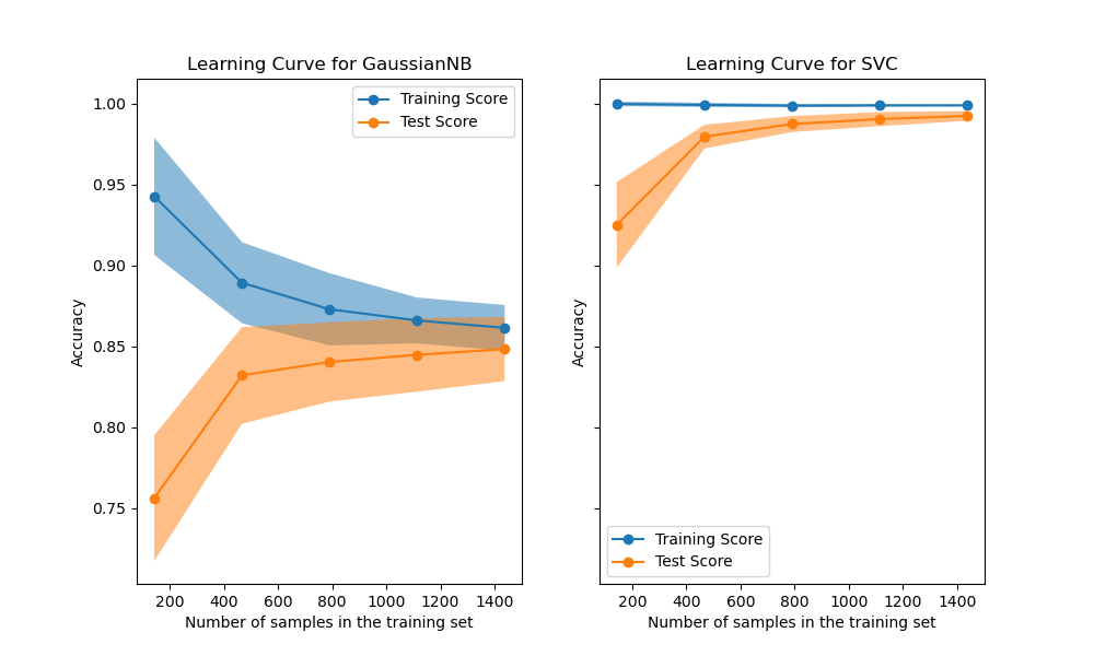
As usual, the scikit-learn developers do a great job explaining the concept in addition to providing a great library. I encourage you to follow that link. This gist is that—for some models on some datasets—training the model on more observations doesn’t improve performance. At some point the learning curve levels off and you’re just wasting time and money training on those extra observations.
For today, we’ll assume that we’re on the flat part of the learning curve. Later in the series we’ll explore cases where we run out of RAM before the learning curve levels off.
Fit, Predict
In my experience, the first place I bump into RAM constraints is when my training dataset fits in memory, but I have to make predictions for a dataset that’s orders of magnitude larger. In these cases, I fit my model like normal, and do my predictions out-of-core (without reading the full dataset into memory at once).
We’ll see that the training side is completely normal (since everything fits in RAM). We’ll see that dask let’s us write normal-looking pandas and NumPy code, so we don’t have to worry about writing the batching code ourself.
To make this concrete, we’ll use the (tried and true) New York City taxi dataset. The goal will be to predict if the passenger leaves a tip. We’ll train the model on a single month’s worth of data (which fits in my laptop’s RAM), and predict on the full dataset2.
Let’s load in the first month of data from disk:
dtype = {
    'vendor_name': 'category',
    'Payment_Type': 'category',
}

df = pd.read_csv("data/yellow_tripdata_2009-01.csv", dtype=dtype,
                 parse_dates=['Trip_Pickup_DateTime', 'Trip_Dropoff_DateTime'],)
df.head()
| vendor_name | Trip_Pickup_DateTime | Trip_Dropoff_DateTime | Passenger_Count | Trip_Distance | Start_Lon | Start_Lat | Rate_Code | store_and_forward | End_Lon | End_Lat | Payment_Type | Fare_Amt | surcharge | mta_tax | Tip_Amt | Tolls_Amt | Total_Amt | |
|---|---|---|---|---|---|---|---|---|---|---|---|---|---|---|---|---|---|---|
| 0 | VTS | 2009-01-04 02:52:00 | 2009-01-04 03:02:00 | 1 | 2.63 | -73.991957 | 40.721567 | NaN | NaN | -73.993803 | 40.695922 | CASH | 8.9 | 0.5 | NaN | 0.00 | 0.0 | 9.40 |
| 1 | VTS | 2009-01-04 03:31:00 | 2009-01-04 03:38:00 | 3 | 4.55 | -73.982102 | 40.736290 | NaN | NaN | -73.955850 | 40.768030 | Credit | 12.1 | 0.5 | NaN | 2.00 | 0.0 | 14.60 |
| 2 | VTS | 2009-01-03 15:43:00 | 2009-01-03 15:57:00 | 5 | 10.35 | -74.002587 | 40.739748 | NaN | NaN | -73.869983 | 40.770225 | Credit | 23.7 | 0.0 | NaN | 4.74 | 0.0 | 28.44 |
| 3 | DDS | 2009-01-01 20:52:58 | 2009-01-01 21:14:00 | 1 | 5.00 | -73.974267 | 40.790955 | NaN | NaN | -73.996558 | 40.731849 | CREDIT | 14.9 | 0.5 | NaN | 3.05 | 0.0 | 18.45 |
| 4 | DDS | 2009-01-24 16:18:23 | 2009-01-24 16:24:56 | 1 | 0.40 | -74.001580 | 40.719382 | NaN | NaN | -74.008378 | 40.720350 | CASH | 3.7 | 0.0 | NaN | 0.00 | 0.0 | 3.70 |
The January 2009 file has about 14M rows, and pandas takes about a minute to read the CSV into memory. We’ll do the usual train-test split:
X = df.drop("Tip_Amt", axis=1)
y = df['Tip_Amt'] > 0

X_train, X_test, y_train, y_test = train_test_split(X, y)

print("Train:", len(X_train))
print("Test: ", len(X_test))
Train: 10569309
Test:  3523104
Aside on Pipelines
The first time you’re introduced to scikit-learn, you’ll typically be shown how
you pass two NumPy arrays X and y straight into an estimator’s .fit
method.
from sklearn.linear_model import LinearRegression

est = LinearRegression()
est.fit(X, y)
Eventually, you might want to use some of scikit-learn’s pre-processing methods.
For example, we might impute missing values with the median and normalize the
data before handing it off to LinearRegression. You could do this “by hand”:
from sklearn.preprocessing import Imputer, StandardScaler

imputer = Imputer(strategy='median')
X_filled = imputer.fit_transform(X, y)

scaler = StandardScaler()
X_scaled = X_scaler.fit_transform(X_filled, y)

est = LinearRegression()
est.fit(X_scaled, y)
We set up each step, and manually pass the data through: X -> X_filled -> X_scaled.
The downside of this approach is that we now have to remember which
pre-processing steps we did, and in what order. The pipeline from raw data to
fit model is spread across multiple python objects. A better approach is to use
scikit-learn’s Pipeline object.
from sklearn.pipeline import make_pipeline

pipe = make_pipeline(
    Imputer(strategy='median'),
    StandardScaler(),
    LinearRegression()
)
pipe.fit(X, y)
Each step in the pipeline implements the fit, transform, and fit_transform
methods. Scikit-learn takes care of shepherding the data through the various
transforms, and finally to the estimator at the end. Pipelines have many
benefits but the main one for our purpose today is that it packages our entire
task into a single python object. Later on, our predict step will be a single
function call, which makes scaling out to the entire dataset extremely
convenient.
If you want more information on Pipelines, check out the scikit-learn
docs, this blog post, and my talk from
PyData Chicago 2016. We’ll be implementing some custom ones,
which is not the point of this post. Don’t get lost in the weeds here, I only
include this section for completeness.
Our Pipeline
This isn’t a perfectly clean dataset, which is nice because it gives us a chance to demonstrate some pandas’ pre-processing prowess, before we hand the data of to scikit-learn to fit the model.
from sklearn.pipeline import make_pipeline
# We'll use FunctionTransformer for simple transforms
from sklearn.preprocessing import FunctionTransformer
# TransformerMixin gives us fit_transform for free
from sklearn.base import TransformerMixin
There are some minor differences in the spelling on “Payment Type”:
df.Payment_Type.cat.categories
Index(['CASH', 'CREDIT', 'Cash', 'Credit', 'Dispute', 'No Charge'], dtype='object')
We’ll reconcile that by lower-casing everything with a .str.lower(). But
resist the temptation to just do that imperatively inplace! We’ll package it up
into a function that will later be wrapped up in a FunctionTransformer.
def payment_lowerer(X):
    return X.assign(Payment_Type=X.Payment_Type.str.lower())
I should note here that I’m using
.assign
to update the variables since it implicitly copies the data. We don’t want to
be modifying the caller’s data without their consent.
Not all the columns look useful. We could have easily solved this by only reading in the data that we’re actually going to use, but let’s solve it now with another simple transformer:
class ColumnSelector(TransformerMixin):
    "Select `columns` from `X`"
    def __init__(self, columns):
        self.columns = columns

    def fit(self, X, y=None):
        return self

    def transform(self, X, y=None):
        return X[self.columns]
Internally, pandas stores datetimes like Trip_Pickup_DateTime as a 64-bit
integer representing the nanoseconds since some time in the 1600s. If we left
this untransformed, scikit-learn would happily transform that column to its
integer representation, which may not be the most meaningful item to stick in
a linear model for predicting tips. A better feature might the hour of the day:
class HourExtractor(TransformerMixin):
    "Transform each datetime in `columns` to integer hour of the day"
    def __init__(self, columns):
        self.columns = columns

    def fit(self, X, y=None):
        return self

    def transform(self, X, y=None):
        return X.assign(**{col: lambda x: x[col].dt.hour
                           for col in self.columns})
Likewise, we’ll need to ensure the categorical variables (in a statistical
sense) are categorical dtype (in a pandas sense). We want categoricals so that
we can call get_dummies later on without worrying about missing or extra
categories in a subset of the data throwing off our linear algebra (See my
talk for more details).
class CategoricalEncoder(TransformerMixin):
    """
    Convert to Categorical with specific `categories`.

    Examples
    --------
    >>> CategoricalEncoder({"A": ['a', 'b', 'c']}).fit_transform(
    ...     pd.DataFrame({"A": ['a', 'b', 'a', 'a']})
    ... )['A']
    0    a
    1    b
    2    a
    3    a
    Name: A, dtype: category
    Categories (2, object): [a, b, c]
    """
    def __init__(self, categories):
        self.categories = categories

    def fit(self, X, y=None):
        return self

    def transform(self, X, y=None):
        X = X.copy()
        for col, categories in self.categories.items():
            X[col] = X[col].astype('category').cat.set_categories(categories)
        return X
Finally, we’d like to normalize the quantitative subset of the data. Scikit-learn has a StandardScaler, which we’ll mimic here, to just operate on a subset of the columns.
class StandardScaler(TransformerMixin):
    "Scale a subset of the columns in a DataFrame"
    def __init__(self, columns):
        self.columns = columns

    def fit(self, X, y=None):
        # Yes, non-ASCII symbols can be a valid identfiers in python 3
        self.μs = X[self.columns].mean()
        self.σs = X[self.columns].std()
        return self

    def transform(self, X, y=None):
        X = X.copy()
        X[self.columns] = X[self.columns].sub(self.μs).div(self.σs)
        return X
Side-note: I’d like to repeat my desire for a library of Transformers that
work well on NumPy arrays, dask arrays, pandas DataFrames and dask dataframes.
I think that’d be a popular library. Essentially everything we’ve written could
go in there and be imported.
Now we can build up the pipeline:
# The columns at the start of the pipeline
columns = ['vendor_name', 'Trip_Pickup_DateTime',
           'Passenger_Count', 'Trip_Distance',
           'Payment_Type', 'Fare_Amt', 'surcharge']

# The mapping of {column: set of categories}
categories = {
    'vendor_name': ['CMT', 'DDS', 'VTS'],
    'Payment_Type': ['cash', 'credit', 'dispute', 'no charge'],
}

scale = ['Trip_Distance', 'Fare_Amt', 'surcharge']

pipe = make_pipeline(
    ColumnSelector(columns),
    HourExtractor(['Trip_Pickup_DateTime']),
    FunctionTransformer(payment_lowerer, validate=False),
    CategoricalEncoder(categories),
    FunctionTransformer(pd.get_dummies, validate=False),
    StandardScaler(scale),
    LogisticRegression(),
)
pipe
[('columnselector', <__main__.ColumnSelector at 0x1a2c726d8>),
 ('hourextractor', <__main__.HourExtractor at 0x10dc72a90>),
 ('functiontransformer-1', FunctionTransformer(accept_sparse=False,
           func=<function payment_lowerer at 0x17e0d5510>, inv_kw_args=None,
           inverse_func=None, kw_args=None, pass_y='deprecated',
           validate=False)),
 ('categoricalencoder', <__main__.CategoricalEncoder at 0x11dd72f98>),
 ('functiontransformer-2', FunctionTransformer(accept_sparse=False,
           func=<function get_dummies at 0x10f43b0d0>, inv_kw_args=None,
           inverse_func=None, kw_args=None, pass_y='deprecated',
           validate=False)),
 ('standardscaler', <__main__.StandardScaler at 0x162580a90>),
 ('logisticregression',
  LogisticRegression(C=1.0, class_weight=None, dual=False, fit_intercept=True,
           intercept_scaling=1, max_iter=100, multi_class='ovr', n_jobs=1,
           penalty='l2', random_state=None, solver='liblinear', tol=0.0001,
           verbose=0, warm_start=False))]
We can fit the pipeline as normal:
%time pipe.fit(X_train, y_train)
This take about a minute on my laptop. We can check the accuracy (but again, this isn’t the point)
>>> pipe.score(X_train, y_train)
0.9931

>>> pipe.score(X_test, y_test)
0.9931
It turns out people essentially tip if and only if they’re paying with a card, so this isn’t a particularly difficult task. Or perhaps more accurately, tips are only recorded when someone pays with a card.
Scaling Out with Dask
OK, so we’ve fit our model and it’s been basically normal. Maybe we’ve been overly-dogmatic about doing everything in a pipeline, but that’s just good model hygiene anyway.
Now, to scale out to the rest of the dataset. We’ll predict the probability of tipping for every cab ride in the dataset (bearing in mind that the full dataset doesn’t fit in my laptop’s RAM, so we’ll do it out-of-core).
To make things a bit easier we’ll use dask, though it isn’t strictly necessary for this section. It saves us from writing a for loop (big whoop). Later on well see that we can, reuse this code when we go to scale out to a cluster (that part is pretty cool, actually). Dask can scale down to a single laptop, and up to thousands of cores.
import dask.dataframe as dd

df = dd.read_csv("data/*.csv", dtype=dtype,
                 parse_dates=['Trip_Pickup_DateTime', 'Trip_Dropoff_DateTime'],)

X = df.drop("Tip_Amt", axis=1)
X is a dask.dataframe, which can be mostly be treated like a pandas
dataframe (internally, operations are done on many smaller dataframes). X has
about 170M rows (compared with the 14M for the training dataset).
Since scikit-learn isn’t dask-aware, we can’t simply call
pipe.predict_proba(X). At some point, our dask.dataframe would be cast to a
numpy.ndarray, and our memory would blow up. Fortunately, dask has some nice
little escape hatches for dealing with functions that know how to operate on
NumPy arrays, but not dask objects. In this case, we’ll use map_partitions.
yhat = X.map_partitions(lambda x: pd.Series(pipe.predict_proba(x)[:, 1],
                                            name='yhat'),
                        meta=('yhat', 'f8'))
map_partitions will go through each partition in your dataframe (one per
file), calling the function on each partition. Dask worries about stitching
together the result (though we provide a hint with the meta keyword, to say
that it’s a Series with name yhat and dtype f8).
Now we can write it out to disk (using parquet rather than CSV, because CSVs are evil).
yhat.to_frame().to_parquet("data/predictions.parq")
This takes about 9 minutes to finish on my laptop.
Scaling Out (even further)
If 9 minutes is too long, and you happen to have a cluster sitting around, you can repurpose that dask code to run on the distributed scheduler. I’ll use dask-kubernetes, to start up a cluster on Google Cloud Platform, but you could also use dask-ec2 for AWS, or dask-drmaa or dask-yarn if already have access to a cluster from your business or institution.
dask-kubernetes create scalable-ml
This sets up a cluster with 8 workers and 54 GB of memory.
The next part of this post is a bit fuzzy, since your teams will probably have different procedures and infrastructure around persisting models. At my old job, I wrote a small utility for serializing a scikit-learn model along with some metadata about what it was trained on, before dumping it in S3. If you want to be fancy, you should watch this talk by Rob Story on how Stripe handles these things (it’s a bit more sophisticated than my “dump it on S3” script).
For this blog post, “shipping it to prod” consists of a joblib.dump(pipe, "taxi-model.pkl") on our laptop, and copying it to somewhere the cluster can
load the file. Then on the cluster, we’ll load it up, and create a Client to
communicate with our cluster’s workers.
from distributed import Client
from sklearn.externals import joblib

pipe = joblib.load("taxi-model.pkl")
c = Client('dask-scheduler:8786')
Depending on how your cluster is set up, specifically with respect to having a shared-file-system or not, the rest of the code is more-or-less identical. If we’re using S3 or Google Cloud Storage as our shared file system, we’d modify the loading code to read from S3 or GCS, rather than our local hard drive:
df = dd.read_csv("s3://bucket/yellow_tripdata_2009*.csv",
                 dtype=dtype,
                 parse_dates=['Trip_Pickup_DateTime', 'Trip_Dropoff_DateTime'],
                 storage_options={'anon': True})
df = c.persist(df)  # persist the dataset in distributed memory
                    # across all the workers in the Dataset
X = df.drop("Tip_Amt", axis=1)
y = df['Tip_Amt'] > 0
Computing the predictions is identical to our out-of-core-on-my-laptop code:
yhat = X.map_partitions(lambda x: pd.Series(pipe.predict_proba(x)[:, 1], name='yhat'),
                        meta=('yhat', 'f8'))
And saving the data (say to S3) might look like
yhat.to_parquet("s3://bucket/predictions.parq")
The loading took about 4 minutes on the cluster, the predict about 10 seconds, and the writing about 1 minute. Not bad overall.
Wrapup
Today, we went into detail on what’s potentially the first scaling problem you’ll hit with scikit-learn: you can train your dataset in-memory (on a laptop, or a large workstation), but you have to predict on a much larger dataset.
We saw that the existing tools handle this case quite well. For training, we
followed best-practices and did everything inside a Pipeline object. For
predicting, we used dask to write regular pandas code that worked out-of-core
on my laptop or on a distributed cluster.
If this topic interests you, you should watch this talk by Stephen Hoover on how Civis is scaling scikit-learn.
In future posts we’ll dig into
- how dask can speed up your existing pipelines by executing them in parallel
- scikit-learn’s out of core API for when your training dataset doesn’t fit in memory
- using dask to implement distributed machine learning algorithms
Until then I would really appreciate your feedback. My personal experience using scikit-learn and pandas can’t cover the diversity of use-cases they’re being thrown into. You can reach me on Twitter @TomAugspurger or by email at mailto:[email protected]. Thanks for reading!
]]>I’m faced with a fairly specific problem: Compute the pairwise distances between two matrices $X$ and $Y$ as quickly as possible. We’ll assume that $Y$ is fairly small, but $X$ may not fit in memory. This post tracks my progress.
]]>Today I released stitch into the
wild. If you haven’t yet, check out the examples
page to see an example of what stitch does,
and the Github repo for how to
install. I’m using this post to explain why I wrote stitch, and some
issues it tries to solve.
Why knitr / knitpy / stitch / RMarkdown?
Each of these tools or formats have the same high-level goal: produce reproducible, dynamic (to changes in the data) reports. They take some source document (typically markdown) that’s a mixture of text and code and convert it to a destination output (HTML, PDF, docx, etc.).
The main difference from something like pandoc, is that these tools actually execute the code and interweave the output of the code back into the document.
Reproducibility is something I care very deeply about. My workflow when writing a report is typically
- prototype in the notebook or IPython REPL (data cleaning, modeling, visualizing, repeat)
- rewrite and cleanup those prototypes in a
.pyfile that produces one or more outputs (figure, table, parameter, etc.) - Write the prose contextualizing a figure or table in markdown
- Source output artifacts (figure or table) when converting the markdown to the final output
This was fine, but had a lot of overhead, and separated the generated report from the code itself (which is sometimes, but not always, what you want).
Stitch aims to make this a simpler process. You (just) write your code and results all in one file, and call
stitch input.md -o output.pdf
Why not Jupyter Notebooks?
A valid question, but I think misguided. I love the notebook, and I use
it every day for exploratory research. That said, there’s a continuum
between all-text reports, and all-code reports. For reports that have a
higher ratio of text:code, I prefer writing in my comfortable
text-editor (yay spellcheck!) and using stitch / pandoc to compile the
document. For reports that have more code:text, or that are very early
on in their lifecycle, I prefer notebooks. Use the right tool for the
job.
When writing my pandas ebook, I had to jump through hoops to get from notebook source to final output (epub or PDF) that looked OK. NBConvert was essential to that workflow, and I couldn’t have done without it. I hope that the stitch-based workflow is a bit smoother.
If a tool similar to podoc is developed, then we can have transparent conversion between text-files with executable blocks of code and notebooks. Living the dream.
Why python?
While RMarkdown / knitr are great (and way more usable than stitch at
this point), they’re essentially only for R. The support for other
languages (last I checked) is limited to passing a code chunk into the
python command-line executable. All state is lost between code chunks.
Stitch supports any language that implements a Jupyter kernel, which is a lot.
Additionally, when RStudio introduced R
Notebooks, they did so
with their own file format, rather than adopting the Jupyter notebook
format. I assume that they were aware of the choice when going their own
way, and made it for the right reasons. But for these types of tasks
(things creating documents) I prefer language-agnostic tools where
possible. It’s certain that RMarkdown / knitr are better than stitch
right now for rendering .Rmd files. It’s quite likely that they will
always be better at working with R than stitch; specialized tools
exist for a reason.
Misc.
Stitch was heavily inspired by Jan Schulz’s knitpy, so you might want to check that out and see if it fits your needs better. Thanks to Jan for giving guidance on difficulty areas he ran into when writing knitpy.
I wrote stitch in about three weeks of random nights and weekends I had free. I stole time that from family or maintaining pandas. Thanks to my wife and the pandas maintainers for picking up my slack.
The three week thing isn’t a boast. It’s a testament to the rich libraries already available. Stitch simply would not exist if we couldn’t reuse
- pandoc via pypandoc for parsing markdown and converting to the destination output (and for installing pandoc via conda-forge)
- Jupyter for providing kernels as execution contexts and a client for easily communicating with them.
- pandocfilters for wrapping code-chunk output
And of course RMarkdown, knitr, and knitpy for proving that a library like this is useful and giving a design that works.
Stitch is still extremely young. It could benefit from users trying it out, and letting me know what’s working and what isn’t. Please do give it a shot and let me know what you think.
© Tom Augspurger
]]>This is part 7 in my series on writing modern idiomatic pandas.
Timeseries
Pandas started out in the financial world, so naturally it has strong timeseries support.
The first half of this post will look at pandas’ capabilities for manipulating time series data. The second half will discuss modelling time series data with statsmodels.
%matplotlib inline

import os
import numpy as np
import pandas as pd
import pandas_datareader.data as web
import seaborn as sns
import matplotlib.pyplot as plt
sns.set(style='ticks', context='talk')

if int(os.environ.get("MODERN_PANDAS_EPUB", 0)):
    import prep # noqa
Let’s grab some stock data for Goldman Sachs using the pandas-datareader package, which spun off of pandas:
gs = web.DataReader("GS", data_source='yahoo', start='2006-01-01',
                    end='2010-01-01')
gs.head().round(2)
| Open | High | Low | Close | Adj Close | Volume | |
|---|---|---|---|---|---|---|
| Date | ||||||
| 2006-01-03 | 126.70 | 129.44 | 124.23 | 128.87 | 112.34 | 6188700 |
| 2006-01-04 | 127.35 | 128.91 | 126.38 | 127.09 | 110.79 | 4861600 |
| 2006-01-05 | 126.00 | 127.32 | 125.61 | 127.04 | 110.74 | 3717400 |
| 2006-01-06 | 127.29 | 129.25 | 127.29 | 128.84 | 112.31 | 4319600 |
| 2006-01-09 | 128.50 | 130.62 | 128.00 | 130.39 | 113.66 | 4723500 |
There isn’t a special data-container just for time series in pandas, they’re just Series or DataFrames with a DatetimeIndex.
Special Slicing
Looking at the elements of gs.index, we see that DatetimeIndexes are made up of pandas.Timestamps:
Looking at the elements of gs.index, we see that DatetimeIndexes are made up of pandas.Timestamps:
gs.index[0]
Timestamp('2006-01-03 00:00:00')
A Timestamp is mostly compatible with the datetime.datetime class, but much amenable to storage in arrays.
Working with Timestamps can be awkward, so Series and DataFrames with DatetimeIndexes have some special slicing rules.
The first special case is partial-string indexing. Say we wanted to select all the days in 2006. Even with Timestamp’s convenient constructors, it’s a pai
gs.loc[pd.Timestamp('2006-01-01'):pd.Timestamp('2006-12-31')].head()
| Open | High | Low | Close | Adj Close | Volume | |
|---|---|---|---|---|---|---|
| Date | ||||||
| 2006-01-03 | 126.699997 | 129.440002 | 124.230003 | 128.869995 | 112.337547 | 6188700 |
| 2006-01-04 | 127.349998 | 128.910004 | 126.379997 | 127.089996 | 110.785889 | 4861600 |
| 2006-01-05 | 126.000000 | 127.320000 | 125.610001 | 127.040001 | 110.742340 | 3717400 |
| 2006-01-06 | 127.290001 | 129.250000 | 127.290001 | 128.839996 | 112.311401 | 4319600 |
| 2006-01-09 | 128.500000 | 130.619995 | 128.000000 | 130.389999 | 113.662605 | 4723500 |
Thanks to partial-string indexing, it’s as simple as
gs.loc['2006'].head()
| Open | High | Low | Close | Adj Close | Volume | |
|---|---|---|---|---|---|---|
| Date | ||||||
| 2006-01-03 | 126.699997 | 129.440002 | 124.230003 | 128.869995 | 112.337547 | 6188700 |
| 2006-01-04 | 127.349998 | 128.910004 | 126.379997 | 127.089996 | 110.785889 | 4861600 |
| 2006-01-05 | 126.000000 | 127.320000 | 125.610001 | 127.040001 | 110.742340 | 3717400 |
| 2006-01-06 | 127.290001 | 129.250000 | 127.290001 | 128.839996 | 112.311401 | 4319600 |
| 2006-01-09 | 128.500000 | 130.619995 | 128.000000 | 130.389999 | 113.662605 | 4723500 |
Since label slicing is inclusive, this slice selects any observation where the year is 2006.
The second “convenience” is __getitem__ (square-bracket) fall-back indexing. I’m only going to mention it here, with the caveat that you should never use it.
DataFrame __getitem__ typically looks in the column: gs['2006'] would search gs.columns for '2006', not find it, and raise a KeyError. But DataFrames with a DatetimeIndex catch that KeyError and try to slice the index.
If it succeeds in slicing the index, the result like gs.loc['2006'] is returned.
If it fails, the KeyError is re-raised.
This is confusing because in pretty much every other case DataFrame.__getitem__ works on columns, and it’s fragile because if you happened to have a column '2006' you would get just that column, and no fall-back indexing would occur. Just use gs.loc['2006'] when slicing DataFrame indexes.
Special Methods
Resampling
Resampling is similar to a groupby: you split the time series into groups (5-day buckets below), apply a function to each group (mean), and combine the result (one row per group).
gs.resample("5d").mean().head()
| Open | High | Low | Close | Adj Close | Volume | |
|---|---|---|---|---|---|---|
| Date | ||||||
| 2006-01-03 | 126.834999 | 128.730002 | 125.877501 | 127.959997 | 111.544294 | 4.771825e+06 |
| 2006-01-08 | 130.349998 | 132.645000 | 130.205002 | 131.660000 | 114.769649 | 4.664300e+06 |
| 2006-01-13 | 131.510002 | 133.395005 | 131.244995 | 132.924995 | 115.872357 | 3.258250e+06 |
| 2006-01-18 | 132.210002 | 133.853333 | 131.656667 | 132.543335 | 115.611125 | 4.997767e+06 |
| 2006-01-23 | 133.771997 | 136.083997 | 133.310001 | 135.153998 | 118.035918 | 3.968500e+06 |
gs.resample("W").agg(['mean', 'sum']).head()
| Open | High | Low | Close | Adj Close | Volume | |||||||
|---|---|---|---|---|---|---|---|---|---|---|---|---|
| mean | sum | mean | sum | mean | sum | mean | sum | mean | sum | mean | sum | |
| Date | ||||||||||||
| 2006-01-08 | 126.834999 | 507.339996 | 128.730002 | 514.920006 | 125.877501 | 503.510002 | 127.959997 | 511.839988 | 111.544294 | 446.177177 | 4771825.0 | 19087300 |
| 2006-01-15 | 130.684000 | 653.419998 | 132.848001 | 664.240006 | 130.544000 | 652.720001 | 131.979999 | 659.899994 | 115.048592 | 575.242958 | 4310420.0 | 21552100 |
| 2006-01-22 | 131.907501 | 527.630005 | 133.672501 | 534.690003 | 131.389999 | 525.559998 | 132.555000 | 530.220000 | 115.603432 | 462.413728 | 4653725.0 | 18614900 |
| 2006-01-29 | 133.771997 | 668.859986 | 136.083997 | 680.419983 | 133.310001 | 666.550003 | 135.153998 | 675.769989 | 118.035918 | 590.179588 | 3968500.0 | 19842500 |
| 2006-02-05 | 140.900000 | 704.500000 | 142.467999 | 712.339996 | 139.937998 | 699.689988 | 141.618002 | 708.090011 | 123.681204 | 618.406020 | 3920120.0 | 19600600 |
You can up-sample to convert to a higher frequency. The new points are filled with NaNs.
gs.resample("6H").mean().head()
| Open | High | Low | Close | Adj Close | Volume | |
|---|---|---|---|---|---|---|
| Date | ||||||
| 2006-01-03 00:00:00 | 126.699997 | 129.440002 | 124.230003 | 128.869995 | 112.337547 | 6188700.0 |
| 2006-01-03 06:00:00 | NaN | NaN | NaN | NaN | NaN | NaN |
| 2006-01-03 12:00:00 | NaN | NaN | NaN | NaN | NaN | NaN |
| 2006-01-03 18:00:00 | NaN | NaN | NaN | NaN | NaN | NaN |
| 2006-01-04 00:00:00 | 127.349998 | 128.910004 | 126.379997 | 127.089996 | 110.785889 | 4861600.0 |
Rolling / Expanding / EW
These methods aren’t unique to DatetimeIndexes, but they often make sense with time series, so I’ll show them here.
gs.Close.plot(label='Raw')
gs.Close.rolling(28).mean().plot(label='28D MA')
gs.Close.expanding().mean().plot(label='Expanding Average')
gs.Close.ewm(alpha=0.03).mean().plot(label='EWMA($\\alpha=.03$)')

plt.legend(bbox_to_anchor=(1.25, .5))
plt.tight_layout()
plt.ylabel("Close ($)")
sns.despine()

Each of .rolling, .expanding, and .ewm return a deferred object, similar to a GroupBy.
roll = gs.Close.rolling(30, center=True)
roll
Rolling [window=30,center=True,axis=0]
m = roll.agg(['mean', 'std'])
ax = m['mean'].plot()
ax.fill_between(m.index, m['mean'] - m['std'], m['mean'] + m['std'],
                alpha=.25)
plt.tight_layout()
plt.ylabel("Close ($)")
sns.despine()

Grab Bag
Offsets
These are similar to dateutil.relativedelta, but works with arrays.
gs.index + pd.DateOffset(months=3, days=-2)
DatetimeIndex(['2006-04-01', '2006-04-02', '2006-04-03', '2006-04-04',
               '2006-04-07', '2006-04-08', '2006-04-09', '2006-04-10',
               '2006-04-11', '2006-04-15',
               ...
               '2010-03-15', '2010-03-16', '2010-03-19', '2010-03-20',
               '2010-03-21', '2010-03-22', '2010-03-26', '2010-03-27',
               '2010-03-28', '2010-03-29'],
              dtype='datetime64[ns]', name='Date', length=1007, freq=None)
Holiday Calendars
There are a whole bunch of special calendars, useful for traders probabaly.
from pandas.tseries.holiday import USColumbusDay
USColumbusDay.dates('2015-01-01', '2020-01-01')
DatetimeIndex(['2015-10-12', '2016-10-10', '2017-10-09', '2018-10-08',
               '2019-10-14'],
              dtype='datetime64[ns]', freq='WOM-2MON')
Timezones
Pandas works with pytz for nice timezone-aware datetimes.
The typical workflow is
- localize timezone-naive timestamps to some timezone
- convert to desired timezone
If you already have timezone-aware Timestamps, there’s no need for step one.
# tz naiive -> tz aware..... to desired UTC
gs.tz_localize('US/Eastern').tz_convert('UTC').head()
| Open | High | Low | Close | Adj Close | Volume | |
|---|---|---|---|---|---|---|
| Date | ||||||
| 2006-01-03 05:00:00+00:00 | 126.699997 | 129.440002 | 124.230003 | 128.869995 | 112.337547 | 6188700 |
| 2006-01-04 05:00:00+00:00 | 127.349998 | 128.910004 | 126.379997 | 127.089996 | 110.785889 | 4861600 |
| 2006-01-05 05:00:00+00:00 | 126.000000 | 127.320000 | 125.610001 | 127.040001 | 110.742340 | 3717400 |
| 2006-01-06 05:00:00+00:00 | 127.290001 | 129.250000 | 127.290001 | 128.839996 | 112.311401 | 4319600 |
| 2006-01-09 05:00:00+00:00 | 128.500000 | 130.619995 | 128.000000 | 130.389999 | 113.662605 | 4723500 |
Modeling Time Series
The rest of this post will focus on time series in the econometric sense. My indented reader for this section isn’t all that clear, so I apologize upfront for any sudden shifts in complexity. I’m roughly targeting material that could be presented in a first or second semester applied statisctics course. What follows certainly isn’t a replacement for that. Any formality will be restricted to footnotes for the curious. I’ve put a whole bunch of resources at the end for people earger to learn more.
We’ll focus on modelling Average Monthly Flights. Let’s download the data. If you’ve been following along in the series, you’ve seen most of this code before, so feel free to skip.
import os
import io
import glob
import zipfile
from utils import download_timeseries

import statsmodels.api as sm


def download_many(start, end):
    months = pd.period_range(start, end=end, freq='M')
    # We could easily parallelize this loop.
    for i, month in enumerate(months):
        download_timeseries(month)


def time_to_datetime(df, columns):
    '''
    Combine all time items into datetimes.

    2014-01-01,1149.0 -> 2014-01-01T11:49:00
    '''
    def converter(col):
        timepart = (col.astype(str)
                       .str.replace('\.0$', '')  # NaNs force float dtype
                       .str.pad(4, fillchar='0'))
        return  pd.to_datetime(df['fl_date'] + ' ' +
                               timepart.str.slice(0, 2) + ':' +
                               timepart.str.slice(2, 4),
                               errors='coerce')
        return datetime_part
    df[columns] = df[columns].apply(converter)
    return df


def read_one(fp):
    df = (pd.read_csv(fp, encoding='latin1')
            .rename(columns=str.lower)
            .drop('unnamed: 6', axis=1)
            .pipe(time_to_datetime, ['dep_time', 'arr_time', 'crs_arr_time',
                                     'crs_dep_time'])
            .assign(fl_date=lambda x: pd.to_datetime(x['fl_date'])))
    return df
/Users/taugspurger/miniconda3/envs/modern-pandas/lib/python3.6/site-packages/statsmodels/compat/pandas.py:56: FutureWarning: The pandas.core.datetools module is deprecated and will be removed in a future version. Please use the pandas.tseries module instead.
  from pandas.core import datetools
store = 'data/ts.hdf5'

if not os.path.exists(store):
    download_many('2000-01-01', '2016-01-01')

    zips = glob.glob(os.path.join('data', 'timeseries', '*.zip'))
    csvs = [unzip_one(fp) for fp in zips]
    dfs = [read_one(fp) for fp in csvs]
    df = pd.concat(dfs, ignore_index=True)

    df['origin'] = df['origin'].astype('category')
    df.to_hdf(store, 'ts', format='table')
else:
    df = pd.read_hdf(store, 'ts')
with pd.option_context('display.max_rows', 100):
    print(df.dtypes)
fl_date         datetime64[ns]
origin                category
crs_dep_time    datetime64[ns]
dep_time        datetime64[ns]
crs_arr_time    datetime64[ns]
arr_time        datetime64[ns]
dtype: object
We can calculate the historical values with a resample.
daily = df.fl_date.value_counts().sort_index()
y = daily.resample('MS').mean()
y.head()
2000-01-01    15176.677419
2000-02-01    15327.551724
2000-03-01    15578.838710
2000-04-01    15442.100000
2000-05-01    15448.677419
Freq: MS, Name: fl_date, dtype: float64
Note that I use the "MS" frequency code there.
Pandas defaults to end of month (or end of year).
Append an 'S' to get the start.
ax = y.plot()
ax.set(ylabel='Average Monthly Flights')
sns.despine()

import statsmodels.formula.api as smf
import statsmodels.tsa.api as smt
import statsmodels.api as sm
One note of warning: I’m using the development version of statsmodels (commit de15ec8 to be precise).
Not all of the items I’ve shown here are available in the currently-released version.
Think back to a typical regression problem, ignoring anything to do with time series for now. The usual task is to predict some value $y$ using some a linear combination of features in $X$.
$$y = \beta_0 + \beta_1 X_1 + \ldots + \beta_p X_p + \epsilon$$
When working with time series, some of the most important (and sometimes only) features are the previous, or lagged, values of $y$.
Let’s start by trying just that “manually”: running a regression of y on lagged values of itself.
We’ll see that this regression suffers from a few problems: multicollinearity, autocorrelation, non-stationarity, and seasonality.
I’ll explain what each of those are in turn and why they’re problems.
Afterwards, we’ll use a second model, seasonal ARIMA, which handles those problems for us.
First, let’s create a dataframe with our lagged values of y using the .shift method, which shifts the index i periods, so it lines up with that observation.
X = (pd.concat([y.shift(i) for i in range(6)], axis=1,
               keys=['y'] + ['L%s' % i for i in range(1, 6)])
       .dropna())
X.head()
| y | L1 | L2 | L3 | L4 | L5 | |
|---|---|---|---|---|---|---|
| 2000-06-01 | 15703.333333 | 15448.677419 | 15442.100000 | 15578.838710 | 15327.551724 | 15176.677419 |
| 2000-07-01 | 15591.677419 | 15703.333333 | 15448.677419 | 15442.100000 | 15578.838710 | 15327.551724 |
| 2000-08-01 | 15850.516129 | 15591.677419 | 15703.333333 | 15448.677419 | 15442.100000 | 15578.838710 |
| 2000-09-01 | 15436.566667 | 15850.516129 | 15591.677419 | 15703.333333 | 15448.677419 | 15442.100000 |
| 2000-10-01 | 15669.709677 | 15436.566667 | 15850.516129 | 15591.677419 | 15703.333333 | 15448.677419 |
We can fit the lagged model using statsmodels (which uses patsy to translate the formula string to a design matrix).
mod_lagged = smf.ols('y ~ trend + L1 + L2 + L3 + L4 + L5',
                     data=X.assign(trend=np.arange(len(X))))
res_lagged = mod_lagged.fit()
res_lagged.summary()
| Dep. Variable: | y | R-squared: | 0.896 |
|---|---|---|---|
| Model: | OLS | Adj. R-squared: | 0.893 |
| Method: | Least Squares | F-statistic: | 261.1 |
| Date: | Sun, 03 Sep 2017 | Prob (F-statistic): | 2.61e-86 |
| Time: | 11:21:46 | Log-Likelihood: | -1461.2 |
| No. Observations: | 188 | AIC: | 2936. |
| Df Residuals: | 181 | BIC: | 2959. |
| Df Model: | 6 | ||
| Covariance Type: | nonrobust |
| coef | std err | t | P>|t| | [0.025 | 0.975] | |
|---|---|---|---|---|---|---|
| Intercept | 1055.4443 | 459.096 | 2.299 | 0.023 | 149.575 | 1961.314 |
| trend | -1.0395 | 0.795 | -1.307 | 0.193 | -2.609 | 0.530 |
| L1 | 1.0143 | 0.075 | 13.543 | 0.000 | 0.867 | 1.162 |
| L2 | -0.0769 | 0.106 | -0.725 | 0.470 | -0.286 | 0.133 |
| L3 | -0.0666 | 0.106 | -0.627 | 0.531 | -0.276 | 0.143 |
| L4 | 0.1311 | 0.106 | 1.235 | 0.219 | -0.078 | 0.341 |
| L5 | -0.0567 | 0.075 | -0.758 | 0.449 | -0.204 | 0.091 |
| Omnibus: | 74.709 | Durbin-Watson: | 1.979 |
|---|---|---|---|
| Prob(Omnibus): | 0.000 | Jarque-Bera (JB): | 851.300 |
| Skew: | 1.114 | Prob(JB): | 1.39e-185 |
| Kurtosis: | 13.184 | Cond. No. | 4.24e+05 |
There are a few problems with this approach though. Since our lagged values are highly correlated with each other, our regression suffers from multicollinearity. That ruins our estimates of the slopes.
sns.heatmap(X.corr());

Second, we’d intuitively expect the $\beta_i$s to gradually decline to zero. The immediately preceding period should be most important ($\beta_1$ is the largest coefficient in absolute value), followed by $\beta_2$, and $\beta_3$… Looking at the regression summary and the bar graph below, this isn’t the case (the cause is related to multicollinearity).
ax = res_lagged.params.drop(['Intercept', 'trend']).plot.bar(rot=0)
plt.ylabel('Coefficeint')
sns.despine()

Finally, our degrees of freedom drop since we lose two for each variable (one for estimating the coefficient, one for the lost observation as a result of the shift).
At least in (macro)econometrics, each observation is precious and we’re loath to throw them away, though sometimes that’s unavoidable.
Autocorrelation
Another problem our lagged model suffered from is autocorrelation (also know as serial correlation).
Roughly speaking, autocorrelation is when there’s a clear pattern in the residuals of your regression (the observed minus the predicted).
Let’s fit a simple model of $y = \beta_0 + \beta_1 T + \epsilon$, where T is the time trend (np.arange(len(y))).
# `Results.resid` is a Series of residuals: y - ŷ
mod_trend = sm.OLS.from_formula(
    'y ~ trend', data=y.to_frame(name='y')
                       .assign(trend=np.arange(len(y))))
res_trend = mod_trend.fit()
Residuals (the observed minus the expected, or $\hat{e_t} = y_t - \hat{y_t}$) are supposed to be white noise. That’s one of the assumptions many of the properties of linear regression are founded upon. In this case there’s a correlation between one residual and the next: if the residual at time $t$ was above expectation, then the residual at time $t + 1$ is much more likely to be above average as well ($e_t > 0 \implies E_t[e_{t+1}] > 0$).
We’ll define a helper function to plot the residuals time series, and some diagnostics about them.
def tsplot(y, lags=None, figsize=(10, 8)):
    fig = plt.figure(figsize=figsize)
    layout = (2, 2)
    ts_ax = plt.subplot2grid(layout, (0, 0), colspan=2)
    acf_ax = plt.subplot2grid(layout, (1, 0))
    pacf_ax = plt.subplot2grid(layout, (1, 1))

    y.plot(ax=ts_ax)
    smt.graphics.plot_acf(y, lags=lags, ax=acf_ax)
    smt.graphics.plot_pacf(y, lags=lags, ax=pacf_ax)
    [ax.set_xlim(1.5) for ax in [acf_ax, pacf_ax]]
    sns.despine()
    plt.tight_layout()
    return ts_ax, acf_ax, pacf_ax
Calling it on the residuals from the linear trend:
tsplot(res_trend.resid, lags=36);

The top subplot shows the time series of our residuals $e_t$, which should be white noise (but it isn’t). The bottom shows the autocorrelation of the residuals as a correlogram. It measures the correlation between a value and it’s lagged self, e.g. $corr(e_t, e_{t-1}), corr(e_t, e_{t-2}), \ldots$. The partial autocorrelation plot in the bottom-right shows a similar concept. It’s partial in the sense that the value for $corr(e_t, e_{t-k})$ is the correlation between those two periods, after controlling for the values at all shorter lags.
Autocorrelation is a problem in regular regressions like above, but we’ll use it to our advantage when we setup an ARIMA model below. The basic idea is pretty sensible: if your regression residuals have a clear pattern, then there’s clearly some structure in the data that you aren’t taking advantage of. If a positive residual today means you’ll likely have a positive residual tomorrow, why not incorporate that information into your forecast, and lower your forecasted value for tomorrow? That’s pretty much what ARIMA does.
It’s important that your dataset be stationary, otherwise you run the risk of finding spurious correlations. A common example is the relationship between number of TVs per person and life expectancy. It’s not likely that there’s an actual causal relationship there. Rather, there could be a third variable that’s driving both (wealth, say). Granger and Newbold (1974) had some stern words for the econometrics literature on this.
We find it very curious that whereas virtually every textbook on econometric methodology contains explicit warnings of the dangers of autocorrelated errors, this phenomenon crops up so frequently in well-respected applied work.
(:fire:), but in that academic passive-aggressive way.
The typical way to handle non-stationarity is to difference the non-stationary variable until is is stationary.
y.to_frame(name='y').assign(Δy=lambda x: x.y.diff()).plot(subplots=True)
sns.despine()

Our original series actually doesn’t look that bad. It doesn’t look like nominal GDP say, where there’s a clearly rising trend. But we have more rigorous methods for detecting whether a series is non-stationary than simply plotting and squinting at it. One popular method is the Augmented Dickey-Fuller test. It’s a statistical hypothesis test that roughly says:
$H_0$ (null hypothesis): $y$ is non-stationary, needs to be differenced
$H_A$ (alternative hypothesis): $y$ is stationary, doesn’t need to be differenced
I don’t want to get into the weeds on exactly what the test statistic is, and what the distribution looks like.
This is implemented in statsmodels as smt.adfuller.
The return type is a bit busy for me, so we’ll wrap it in a namedtuple.
from collections import namedtuple

ADF = namedtuple("ADF", "adf pvalue usedlag nobs critical icbest")
ADF(*smt.adfuller(y))._asdict()
OrderedDict([('adf', -1.3206520699512339),
             ('pvalue', 0.61967180643147923),
             ('usedlag', 15),
             ('nobs', 177),
             ('critical',
              {'1%': -3.4678453197999071,
               '10%': -2.575551186759871,
               '5%': -2.8780117454974392}),
             ('icbest', 2710.6120408261486)])
So we failed to reject the null hypothesis that the original series was non-stationary. Let’s difference it.
ADF(*smt.adfuller(y.diff().dropna()))._asdict()
OrderedDict([('adf', -3.6412428797327996),
             ('pvalue', 0.0050197770854934548),
             ('usedlag', 14),
             ('nobs', 177),
             ('critical',
              {'1%': -3.4678453197999071,
               '10%': -2.575551186759871,
               '5%': -2.8780117454974392}),
             ('icbest', 2696.3891181091631)])
This looks better. It’s not statistically significant at the 5% level, but who cares what statisticins say anyway.
We’ll fit another OLS model of $\Delta y = \beta_0 + \beta_1 L \Delta y_{t-1} + e_t$
data = (y.to_frame(name='y')
         .assign(Δy=lambda df: df.y.diff())
         .assign(LΔy=lambda df: df.Δy.shift()))
mod_stationary = smf.ols('Δy ~ LΔy', data=data.dropna())
res_stationary = mod_stationary.fit()
tsplot(res_stationary.resid, lags=24);

So we’ve taken care of multicolinearity, autocorelation, and stationarity, but we still aren’t done.
Seasonality
We have strong monthly seasonality:
smt.seasonal_decompose(y).plot();

There are a few ways to handle seasonality.
We’ll just rely on the SARIMAX method to do it for us.
For now, recognize that it’s a problem to be solved.
ARIMA
So, we’ve sketched the problems with regular old regression: multicollinearity, autocorrelation, non-stationarity, and seasonality.
Our tool of choice, smt.SARIMAX, which stands for Seasonal ARIMA with eXogenous regressors, can handle all these.
We’ll walk through the components in pieces.
ARIMA stands for AutoRegressive Integrated Moving Average. It’s a relatively simple yet flexible way of modeling univariate time series. It’s made up of three components, and is typically written as $\mathrm{ARIMA}(p, d, q)$.
ARIMA stands for AutoRegressive Integrated Moving Average, and it’s a relatively simple way of modeling univariate time series. It’s made up of three components, and is typically written as $\mathrm{ARIMA}(p, d, q)$.
AutoRegressive
The idea is to predict a variable by a linear combination of its lagged values (auto-regressive as in regressing a value on its past self). An AR(p), where $p$ represents the number of lagged values used, is written as
$$y_t = c + \phi_1 y_{t-1} + \phi_2 y_{t-2} + \ldots + \phi_p y_{t-p} + e_t$$
$c$ is a constant and $e_t$ is white noise. This looks a lot like a linear regression model with multiple predictors, but the predictors happen to be lagged values of $y$ (though they are estimated differently).
Integrated
Integrated is like the opposite of differencing, and is the part that deals with stationarity. If you have to difference your dataset 1 time to get it stationary, then $d=1$. We’ll introduce one bit of notation for differencing: $\Delta y_t = y_t - y_{t-1}$ for $d=1$.
Moving Average
MA models look somewhat similar to the AR component, but it’s dealing with different values.
$$y_t = c + e_t + \theta_1 e_{t-1} + \theta_2 e_{t-2} + \ldots + \theta_q e_{t-q}$$
$c$ again is a constant and $e_t$ again is white noise. But now the coefficients are the residuals from previous predictions.
Combining
Putting that together, an ARIMA(1, 1, 1) process is written as
$$\Delta y_t = c + \phi_1 \Delta y_{t-1} + \theta_t e_{t-1} + e_t$$
Using lag notation, where $L y_t = y_{t-1}$, i.e. y.shift() in pandas, we can rewrite that as
$$(1 - \phi_1 L) (1 - L)y_t = c + (1 + \theta L)e_t$$
That was for our specific $\mathrm{ARIMA}(1, 1, 1)$ model. For the general $\mathrm{ARIMA}(p, d, q)$, that becomes
$$(1 - \phi_1 L - \ldots - \phi_p L^p) (1 - L)^d y_t = c + (1 + \theta L + \ldots + \theta_q L^q)e_t$$
We went through that extremely quickly, so don’t feel bad if things aren’t clear. Fortunately, the model is pretty easy to use with statsmodels (using it correctly, in a statistical sense, is another matter).
mod = smt.SARIMAX(y, trend='c', order=(1, 1, 1))
res = mod.fit()
tsplot(res.resid[2:], lags=24);

res.summary()
| Dep. Variable: | fl_date | No. Observations: | 193 |
|---|---|---|---|
| Model: | SARIMAX(1, 1, 1) | Log Likelihood | -1494.618 |
| Date: | Sun, 03 Sep 2017 | AIC | 2997.236 |
| Time: | 11:21:50 | BIC | 3010.287 |
| Sample: | 01-01-2000 | HQIC | 3002.521 |
| - 01-01-2016 | |||
| Covariance Type: | opg |
| coef | std err | z | P>|z| | [0.025 | 0.975] | |
|---|---|---|---|---|---|---|
| intercept | -5.4306 | 66.818 | -0.081 | 0.935 | -136.391 | 125.529 |
| ar.L1 | -0.0327 | 2.689 | -0.012 | 0.990 | -5.303 | 5.237 |
| ma.L1 | 0.0775 | 2.667 | 0.029 | 0.977 | -5.149 | 5.305 |
| sigma2 | 3.444e+05 | 1.69e+04 | 20.392 | 0.000 | 3.11e+05 | 3.77e+05 |
| Ljung-Box (Q): | 225.58 | Jarque-Bera (JB): | 1211.00 |
|---|---|---|---|
| Prob(Q): | 0.00 | Prob(JB): | 0.00 |
| Heteroskedasticity (H): | 0.67 | Skew: | 1.20 |
| Prob(H) (two-sided): | 0.12 | Kurtosis: | 15.07 |
There’s a bunch of output there with various tests, estimated parameters, and information criteria. Let’s just say that things are looking better, but we still haven’t accounted for seasonality.
A seasonal ARIMA model is written as $\mathrm{ARIMA}(p,d,q)×(P,D,Q)_s$. Lowercase letters are for the non-seasonal component, just like before. Upper-case letters are a similar specification for the seasonal component, where $s$ is the periodicity (4 for quarterly, 12 for monthly).
It’s like we have two processes, one for non-seasonal component and one for seasonal components, and we multiply them together with regular algebra rules.
The general form of that looks like (quoting the statsmodels docs here)
$$\phi_p(L)\tilde{\phi}_P(L^S)\Delta^d\Delta_s^D y_t = A(t) + \theta_q(L)\tilde{\theta}_Q(L^s)e_t$$
where
- $\phi_p(L)$ is the non-seasonal autoregressive lag polynomial
- $\tilde{\phi}_P(L^S)$ is the seasonal autoregressive lag polynomial
- $\Delta^d\Delta_s^D$ is the time series, differenced $d$ times, and seasonally differenced $D$ times.
- $A(t)$ is the trend polynomial (including the intercept)
- $\theta_q(L)$ is the non-seasonal moving average lag polynomial
- $\tilde{\theta}_Q(L^s)$ is the seasonal moving average lag polynomial
I don’t find that to be very clear, but maybe an example will help. We’ll fit a seasonal ARIMA$(1,1,2)×(0, 1, 2)_{12}$.
So the nonseasonal component is
- $p=1$: period autoregressive: use $y_{t-1}$
- $d=1$: one first-differencing of the data (one month)
- $q=2$: use the previous two non-seasonal residual, $e_{t-1}$ and $e_{t-2}$, to forecast
And the seasonal component is
- $P=0$: Don’t use any previous seasonal values
- $D=1$: Difference the series 12 periods back:
y.diff(12) - $Q=2$: Use the two previous seasonal residuals
mod_seasonal = smt.SARIMAX(y, trend='c',
                           order=(1, 1, 2), seasonal_order=(0, 1, 2, 12),
                           simple_differencing=False)
res_seasonal = mod_seasonal.fit()
res_seasonal.summary()
| Dep. Variable: | fl_date | No. Observations: | 193 |
|---|---|---|---|
| Model: | SARIMAX(1, 1, 2)x(0, 1, 2, 12) | Log Likelihood | -1357.847 |
| Date: | Sun, 03 Sep 2017 | AIC | 2729.694 |
| Time: | 11:21:53 | BIC | 2752.533 |
| Sample: | 01-01-2000 | HQIC | 2738.943 |
| - 01-01-2016 | |||
| Covariance Type: | opg |
| coef | std err | z | P>|z| | [0.025 | 0.975] | |
|---|---|---|---|---|---|---|
| intercept | -17.5871 | 44.920 | -0.392 | 0.695 | -105.628 | 70.454 |
| ar.L1 | -0.9988 | 0.013 | -74.479 | 0.000 | -1.025 | -0.973 |
| ma.L1 | 0.9956 | 0.109 | 9.130 | 0.000 | 0.782 | 1.209 |
| ma.L2 | 0.0042 | 0.110 | 0.038 | 0.969 | -0.211 | 0.219 |
| ma.S.L12 | -0.7836 | 0.059 | -13.286 | 0.000 | -0.899 | -0.668 |
| ma.S.L24 | 0.2118 | 0.041 | 5.154 | 0.000 | 0.131 | 0.292 |
| sigma2 | 1.842e+05 | 1.21e+04 | 15.240 | 0.000 | 1.61e+05 | 2.08e+05 |
| Ljung-Box (Q): | 32.57 | Jarque-Bera (JB): | 1298.39 |
|---|---|---|---|
| Prob(Q): | 0.79 | Prob(JB): | 0.00 |
| Heteroskedasticity (H): | 0.17 | Skew: | -1.33 |
| Prob(H) (two-sided): | 0.00 | Kurtosis: | 15.89 |
tsplot(res_seasonal.resid[12:], lags=24);

Things look much better now.
One thing I didn’t really talk about is order selection. How to choose $p, d, q, P, D$ and $Q$.
R’s forecast package does have a handy auto.arima function that does this for you.
Python / statsmodels don’t have that at the minute.
The alternative seems to be experience (boo), intuition (boo), and good-old grid-search.
You can fit a bunch of models for a bunch of combinations of the parameters and use the AIC or BIC to choose the best.
Here is a useful reference, and this StackOverflow answer recommends a few options.
Forecasting
Now that we fit that model, let’s put it to use. First, we’ll make a bunch of one-step ahead forecasts. At each point (month), we take the history up to that point and make a forecast for the next month. So the forecast for January 2014 has available all the data up through December 2013.
pred = res_seasonal.get_prediction(start='2001-03-01')
pred_ci = pred.conf_int()
ax = y.plot(label='observed')
pred.predicted_mean.plot(ax=ax, label='Forecast', alpha=.7)
ax.fill_between(pred_ci.index,
                pred_ci.iloc[:, 0],
                pred_ci.iloc[:, 1], color='k', alpha=.2)
ax.set_ylabel("Monthly Flights")
plt.legend()
sns.despine()

There are a few places where the observed series slips outside the 95% confidence interval. The series seems especially unstable before 2005.
Alternatively, we can make dynamic forecasts as of some month (January 2013 in the example below). That means the forecast from that point forward only use information available as of January 2013. The predictions are generated in a similar way: a bunch of one-step forecasts. Only instead of plugging in the actual values beyond January 2013, we plug in the forecast values.
pred_dy = res_seasonal.get_prediction(start='2002-03-01', dynamic='2013-01-01')
pred_dy_ci = pred_dy.conf_int()
ax = y.plot(label='observed')
pred_dy.predicted_mean.plot(ax=ax, label='Forecast')
ax.fill_between(pred_dy_ci.index,
                pred_dy_ci.iloc[:, 0],
                pred_dy_ci.iloc[:, 1], color='k', alpha=.25)
ax.set_ylabel("Monthly Flights")

# Highlight the forecast area
ax.fill_betweenx(ax.get_ylim(), pd.Timestamp('2013-01-01'), y.index[-1],
                 alpha=.1, zorder=-1)
ax.annotate('Dynamic $\\longrightarrow$', (pd.Timestamp('2013-02-01'), 550))

plt.legend()
sns.despine()

Resources
This is a collection of links for those interested.
Time series modeling in Python
General Textbooks
- Forecasting: Principles and Practice: A great introduction
- Stock and Watson: Readable undergraduate resource, has a few chapters on time series
- Greene’s Econometric Analysis: My favorite PhD level textbook
- Hamilton’s Time Series Analysis: A classic
- Lutkehpohl’s New Introduction to Multiple Time Series Analysis: Extremely dry, but useful if you’re implementing this stuff
Conclusion
Congratulations if you made it this far, this piece just kept growing (and I still had to cut stuff).
The main thing cut was talking about how SARIMAX is implemented on top of using statsmodels’ statespace framework.
The statespace framework, developed mostly by Chad Fulton over the past couple years, is really nice.
You can pretty easily extend it with custom models, but still get all the benefits of the framework’s estimation and results facilities.
I’d recommend reading the notebooks.
We also didn’t get to talk at all about Skipper Seabold’s work on VARs, but maybe some other time.
As always, feedback is welcome.
This is part 6 in my series on writing modern idiomatic pandas.
Visualization and Exploratory Analysis
A few weeks ago, the R community went through some hand-wringing about plotting packages. For outsiders (like me) the details aren’t that important, but some brief background might be useful so we can transfer the takeaways to Python. The competing systems are “base R”, which is the plotting system built into the language, and ggplot2, Hadley Wickham’s implementation of the grammar of graphics. For those interested in more details, start with
The most important takeaways are that
- Either system is capable of producing anything the other can
- ggplot2 is usually better for exploratory analysis
Item 2 is not universally agreed upon, and it certainly isn’t true for every type of chart, but we’ll take it as fact for now. I’m not foolish enough to attempt a formal analogy here, like “matplotlib is python’s base R”. But there’s at least a rough comparison: like dplyr/tidyr and ggplot2, the combination of pandas and seaborn allows for fast iteration and exploration. When you need to, you can “drop down” into matplotlib for further refinement.
Overview
Here’s a brief sketch of the plotting landscape as of April 2016. For some reason, plotting tools feel a bit more personal than other parts of this series so far, so I feel the need to blanket this who discussion in a caveat: this is my personal take, shaped by my personal background and tastes. Also, I’m not at all an expert on visualization, just a consumer. For real advice, you should listen to the experts in this area. Take this all with an extra grain or two of salt.
Matplotlib
Matplotlib is an amazing project, and is the foundation of pandas’ built-in plotting and Seaborn. It handles everything from the integration with various drawing backends, to several APIs handling drawing charts or adding and transforming individual glyphs (artists). I’ve found knowing the pyplot API useful. You’re less likely to need things like Transforms or artists, but when you do the documentation is there.
Matplotlib has built up something of a bad reputation for being verbose. I think that complaint is valid, but misplaced. Matplotlib lets you control essentially anything on the figure. An overly-verbose API just means there’s an opportunity for a higher-level, domain specific, package to exist (like seaborn for statistical graphics).
Pandas’ builtin-plotting
DataFrame and Series have a .plot namespace, with various chart types available (line, hist, scatter, etc.).
Pandas objects provide additional metadata that can be used to enhance plots (the Index for a better automatic x-axis then range(n) or Index names as axis labels for example).
And since pandas had fewer backwards-compatibility constraints, it had a bit better default aesthetics. The matplotlib 2.0 release will level this, and pandas has deprecated its custom plotting styles, in favor of matplotlib’s (technically I just broke it when fixing matplotlib 1.5 compatibility, so we deprecated it after the fact).
At this point, I see pandas DataFrame.plot as a useful exploratory tool for quick throwaway plots.
Seaborn
Seaborn, created by Michael Waskom, “provides a high-level interface for drawing attractive statistical graphics.” Seaborn gives a great API for quickly exploring different visual representations of your data. We’ll be focusing on that today
Bokeh
Bokeh is a (still under heavy development) visualiztion library that targets the browser.
Like matplotlib, Bokeh has a few APIs at various levels of abstraction. They have a glyph API, which I suppose is most similar to matplotlib’s Artists API, for drawing single or arrays of glpyhs (circles, rectangles, polygons, etc.). More recently they introduced a Charts API, for producing canned charts from data structures like dicts or DataFrames.
Other Libraries
This is a (probably incomplete) list of other visualization libraries that I don’t know enough about to comment on
It’s also possible to use Javascript tools like D3 directly in the Jupyter notebook, but we won’t go into those today.
Examples
I do want to pause and explain the type of work I’m doing with these packages. The vast majority of plots I create are for exploratory analysis, helping me understand the dataset I’m working with. They aren’t intended for the client (whoever that is) to see. Occasionally that exploratory plot will evolve towards a final product that will be used to explain things to the client. In this case I’ll either polish the exploratory plot, or rewrite it in another system more suitable for the final product (in D3 or Bokeh, say, if it needs to be an interactive document in the browser).
Now that we have a feel for the overall landscape (from my point of view), let’s delve into a few examples.
We’ll use the diamonds dataset from ggplot2.
You could use Vincent Arelbundock’s RDatasets package to find it (pd.read_csv('http://vincentarelbundock.github.io/Rdatasets/csv/ggplot2/diamonds.csv')), but I wanted to checkout feather.
import os
import feather
import numpy as np
import pandas as pd
import matplotlib.pyplot as plt
import seaborn as sns

if int(os.environ.get("MODERN_PANDAS_EPUB", 0)):
    import prep # noqa
%load_ext rpy2.ipython
%%R
suppressPackageStartupMessages(library(ggplot2))
library(feather)
write_feather(diamonds, 'diamonds.fthr')
import feather
df = feather.read_dataframe('diamonds.fthr')
df.head()
| carat | cut | color | clarity | depth | table | price | x | y | z | |
|---|---|---|---|---|---|---|---|---|---|---|
| 0 | 0.23 | Ideal | E | SI2 | 61.5 | 55.0 | 326 | 3.95 | 3.98 | 2.43 |
| 1 | 0.21 | Premium | E | SI1 | 59.8 | 61.0 | 326 | 3.89 | 3.84 | 2.31 |
| 2 | 0.23 | Good | E | VS1 | 56.9 | 65.0 | 327 | 4.05 | 4.07 | 2.31 |
| 3 | 0.29 | Premium | I | VS2 | 62.4 | 58.0 | 334 | 4.20 | 4.23 | 2.63 |
| 4 | 0.31 | Good | J | SI2 | 63.3 | 58.0 | 335 | 4.34 | 4.35 | 2.75 |
df.info()
<class 'pandas.core.frame.DataFrame'>
RangeIndex: 53940 entries, 0 to 53939
Data columns (total 10 columns):
carat      53940 non-null float64
cut        53940 non-null category
color      53940 non-null category
clarity    53940 non-null category
depth      53940 non-null float64
table      53940 non-null float64
price      53940 non-null int32
x          53940 non-null float64
y          53940 non-null float64
z          53940 non-null float64
dtypes: category(3), float64(6), int32(1)
memory usage: 2.8 MB
It’s not clear to me where the scientific community will come down on Bokeh for exploratory analysis. The ability to share interactive graphics is compelling. The trend towards more and more analysis and communication happening in the browser will only enhance this feature of Bokeh.
Personally though, I have a lot of inertia behind matplotlib so I haven’t switched to Bokeh for day-to-day exploratory analysis.
I have greatly enjoyed Bokeh for building dashboards and webapps with Bokeh server. It’s still young, and I’ve hit some rough edges, but I’m happy to put up with some awkwardness to avoid writing more javascript.
sns.set(context='talk', style='ticks')

%matplotlib inline
Matplotlib
Since it’s relatively new, I should point out that matplotlib 1.5 added support for plotting labeled data.
fig, ax = plt.subplots()

ax.scatter(x='carat', y='depth', data=df, c='k', alpha=.15);

This isn’t limited to just DataFrames.
It supports anything that uses __getitem__ (square-brackets) with string keys.
Other than that, I don’t have much to add to the matplotlib documentation.
Pandas Built-in Plotting
The metadata in DataFrames gives a bit better defaults on plots.
df.plot.scatter(x='carat', y='depth', c='k', alpha=.15)
plt.tight_layout()

We get axis labels from the column names. Nothing major, just nice.
Pandas can be more convenient for plotting a bunch of columns with a shared x-axis (the index), say several timeseries.
from pandas_datareader import fred

gdp = fred.FredReader(['GCEC96', 'GPDIC96'], start='2000-01-01').read()

gdp.rename(columns={"GCEC96": "Government Expenditure",
                    "GPDIC96": "Private Investment"}).plot(figsize=(12, 6))
plt.tight_layout()
/Users/taugspurger/miniconda3/envs/modern-pandas/lib/python3.6/site-packages/ipykernel_launcher.py:3: DeprecationWarning: pandas.core.common.is_list_like is deprecated. import from the public API: pandas.api.types.is_list_like instead
  This is separate from the ipykernel package so we can avoid doing imports until

Seaborn
The rest of this post will focus on seaborn, and why I think it’s especially great for exploratory analysis.
I would encourage you to read Seaborn’s introductory notes, which describe its design philosophy and attempted goals. Some highlights:
Seaborn aims to make visualization a central part of exploring and understanding data.
It does this through a consistent, understandable (to me anyway) API.
The plotting functions try to do something useful when called with a minimal set of arguments, and they expose a number of customizable options through additional parameters.
Which works great for exploratory analysis, with the option to turn that into something more polished if it looks promising.
Some of the functions plot directly into a matplotlib axes object, while others operate on an entire figure and produce plots with several panels.
The fact that seaborn is built on matplotlib means that if you are familiar with the pyplot API, your knowledge will still be useful.
Most seaborn plotting functions (one per chart-type) take an x, y, hue, and data arguments (only some are required, depending on the plot type). If you’re working with DataFrames, you’ll pass in strings referring to column names, and the DataFrame for data.
sns.countplot(x='cut', data=df)
sns.despine()
plt.tight_layout()

sns.barplot(x='cut', y='price', data=df)
sns.despine()
plt.tight_layout()

Bivariate relationships can easily be explored, either one at a time:
sns.jointplot(x='carat', y='price', data=df, size=8, alpha=.25,
              color='k', marker='.')
plt.tight_layout()

Or many at once
g = sns.pairplot(df, hue='cut')

pairplot is a convenience wrapper around PairGrid, and offers our first look at an important seaborn abstraction, the Grid. Seaborn Grids provide a link between a matplotlib Figure with multiple axes and features in your dataset.
There are two main ways of interacting with grids. First, seaborn provides convenience-wrapper functions like pairplot, that have good defaults for common tasks. If you need more flexibility, you can work with the Grid directly by mapping plotting functions over each axes.
def core(df, α=.05):
    mask = (df > df.quantile(α)).all(1) & (df < df.quantile(1 - α)).all(1)
    return df[mask]
cmap = sns.cubehelix_palette(as_cmap=True, dark=0, light=1, reverse=True)

(df.select_dtypes(include=[np.number])
   .pipe(core)
   .pipe(sns.PairGrid)
   .map_upper(plt.scatter, marker='.', alpha=.25)
   .map_diag(sns.kdeplot)
   .map_lower(plt.hexbin, cmap=cmap, gridsize=20)
);

This last example shows the tight integration with matplotlib. g.axes is an array of matplotlib.Axes and g.fig is a matplotlib.Figure.
This is a pretty common pattern when using seaborn: use a seaborn plotting method (or grid) to get a good start, and then adjust with matplotlib as needed.
I think (not an expert on this at all) that one thing people like about the grammar of graphics is its flexibility.
You aren’t limited to a fixed set of chart types defined by the library author.
Instead, you construct your chart by layering scales, aesthetics and geometries.
And using ggplot2 in R is a delight.
That said, I wouldn’t really call what seaborn / matplotlib offer that limited. You can create pretty complex charts suited to your needs.
agged = df.groupby(['cut', 'color']).mean().sort_index().reset_index()
g = sns.PairGrid(agged, x_vars=agged.columns[2:], y_vars=['cut', 'color'],
size=5, aspect=.65)
g.map(sns.stripplot, orient="h", size=10, palette='Blues_d');

g = sns.FacetGrid(df, col='color', hue='color', col_wrap=4)
g.map(sns.regplot, 'carat', 'price');

Initially I had many more examples showing off seaborn, but I’ll spare you. Seaborn’s documentation is thorough (and just beautiful to look at).
We’ll end with a nice scikit-learn integration for exploring the parameter-space on a GridSearch object.
from sklearn.ensemble import RandomForestClassifier
from sklearn.model_selection import GridSearchCV
For those unfamiliar with machine learning or scikit-learn, the basic idea is your algorithm (RandomForestClassifer) is trying to maximize some objective function (percent of correctly classified items in this case).
There are various hyperparameters that affect the fit.
We can search this space by trying out a bunch of possible values for each parameter with the GridSearchCV estimator.
df = sns.load_dataset('titanic')
clf = RandomForestClassifier()
param_grid = dict(max_depth=[1, 2, 5, 10, 20, 30, 40],
min_samples_split=[2, 5, 10],
min_samples_leaf=[2, 3, 5])
est = GridSearchCV(clf, param_grid=param_grid, n_jobs=4)
y = df['survived']
X = df.drop(['survived', 'who', 'alive'], axis=1)
X = pd.get_dummies(X, drop_first=True)
X = X.fillna(value=X.median())
est.fit(X, y);
scores = pd.DataFrame(est.cv_results_)
scores.head()
| mean_fit_time | mean_score_time | mean_test_score | mean_train_score | param_max_depth | param_min_samples_leaf | param_min_samples_split | params | rank_test_score | split0_test_score | split0_train_score | split1_test_score | split1_train_score | split2_test_score | split2_train_score | std_fit_time | std_score_time | std_test_score | std_train_score | |
|---|---|---|---|---|---|---|---|---|---|---|---|---|---|---|---|---|---|---|---|
| 0 | 0.017463 | 0.002174 | 0.786756 | 0.797419 | 1 | 2 | 2 | {'max_depth': 1, 'min_samples_leaf': 2, 'min_s... | 54 | 0.767677 | 0.804714 | 0.808081 | 0.797980 | 0.784512 | 0.789562 | 0.000489 | 0.000192 | 0.016571 | 0.006198 |
| 1 | 0.014982 | 0.001843 | 0.773288 | 0.783951 | 1 | 2 | 5 | {'max_depth': 1, 'min_samples_leaf': 2, 'min_s... | 57 | 0.767677 | 0.804714 | 0.754209 | 0.752525 | 0.797980 | 0.794613 | 0.001900 | 0.000356 | 0.018305 | 0.022600 |
| 2 | 0.013890 | 0.001895 | 0.771044 | 0.786195 | 1 | 2 | 10 | {'max_depth': 1, 'min_samples_leaf': 2, 'min_s... | 58 | 0.767677 | 0.811448 | 0.754209 | 0.752525 | 0.791246 | 0.794613 | 0.000935 | 0.000112 | 0.015307 | 0.024780 |
| 3 | 0.015679 | 0.001691 | 0.764310 | 0.760943 | 1 | 3 | 2 | {'max_depth': 1, 'min_samples_leaf': 3, 'min_s... | 61 | 0.801347 | 0.799663 | 0.700337 | 0.695286 | 0.791246 | 0.787879 | 0.001655 | 0.000025 | 0.045423 | 0.046675 |
| 4 | 0.013034 | 0.001695 | 0.765432 | 0.787318 | 1 | 3 | 5 | {'max_depth': 1, 'min_samples_leaf': 3, 'min_s... | 60 | 0.710438 | 0.772727 | 0.801347 | 0.781145 | 0.784512 | 0.808081 | 0.000289 | 0.000038 | 0.039490 | 0.015079 |
sns.factorplot(x='param_max_depth', y='mean_test_score',
col='param_min_samples_split',
hue='param_min_samples_leaf',
data=scores);

Thanks for reading! I want to reiterate at the end that this is just my way of doing data visualization. Your needs might differ, meaning you might need different tools. You can still use pandas to get it to the point where it’s ready to be visualized!
As always, feedback is welcome.
]]>This is part 5 in my series on writing modern idiomatic pandas.
Reshaping & Tidy Data
Structuring datasets to facilitate analysis (Wickham 2014)
So, you’ve sat down to analyze a new dataset. What do you do first?
In episode 11 of Not So Standard Deviations, Hilary and Roger discussed their typical approaches. I’m with Hilary on this one, you should make sure your data is tidy. Before you do any plots, filtering, transformations, summary statistics, regressions… Without a tidy dataset, you’ll be fighting your tools to get the result you need. With a tidy dataset, it’s relatively easy to do all of those.
Hadley Wickham kindly summarized tidiness as a dataset where
- Each variable forms a column
- Each observation forms a row
- Each type of observational unit forms a table
And today we’ll only concern ourselves with the first two. As quoted at the top, this really is about facilitating analysis: going as quickly as possible from question to answer.
%matplotlib inline
import os
import numpy as np
import pandas as pd
import seaborn as sns
import matplotlib.pyplot as plt
if int(os.environ.get("MODERN_PANDAS_EPUB", 0)):
import prep # noqa
pd.options.display.max_rows = 10
sns.set(style='ticks', context='talk')
NBA Data
This StackOverflow question asked about calculating the number of days of rest NBA teams have between games. The answer would have been difficult to compute with the raw data. After transforming the dataset to be tidy, we’re able to quickly get the answer.
We’ll grab some NBA game data from basketball-reference.com using pandas’ read_html function, which returns a list of DataFrames.
fp = 'data/nba.csv'
if not os.path.exists(fp):
tables = pd.read_html("http://www.basketball-reference.com/leagues/NBA_2016_games.html")
games = tables[0]
games.to_csv(fp)
else:
games = pd.read_csv(fp)
games.head()
| Date | Start (ET) | Unnamed: 2 | Visitor/Neutral | PTS | Home/Neutral | PTS.1 | Unnamed: 7 | Notes | |
|---|---|---|---|---|---|---|---|---|---|
| 0 | October | NaN | NaN | NaN | NaN | NaN | NaN | NaN | NaN |
| 1 | Tue, Oct 27, 2015 | 8:00 pm | Box Score | Detroit Pistons | 106.0 | Atlanta Hawks | 94.0 | NaN | NaN |
| 2 | Tue, Oct 27, 2015 | 8:00 pm | Box Score | Cleveland Cavaliers | 95.0 | Chicago Bulls | 97.0 | NaN | NaN |
| 3 | Tue, Oct 27, 2015 | 10:30 pm | Box Score | New Orleans Pelicans | 95.0 | Golden State Warriors | 111.0 | NaN | NaN |
| 4 | Wed, Oct 28, 2015 | 7:30 pm | Box Score | Philadelphia 76ers | 95.0 | Boston Celtics | 112.0 | NaN | NaN |
Side note: pandas’ read_html is pretty good. On simple websites it almost always works.
It provides a couple parameters for controlling what gets selected from the webpage if the defaults fail.
I’ll always use it first, before moving on to BeautifulSoup or lxml if the page is more complicated.
As you can see, we have a bit of general munging to do before tidying. Each month slips in an extra row of mostly NaNs, the column names aren’t too useful, and we have some dtypes to fix up.
column_names = {'Date': 'date', 'Start (ET)': 'start',
'Unamed: 2': 'box', 'Visitor/Neutral': 'away_team',
'PTS': 'away_points', 'Home/Neutral': 'home_team',
'PTS.1': 'home_points', 'Unamed: 7': 'n_ot'}
games = (games.rename(columns=column_names)
.dropna(thresh=4)
[['date', 'away_team', 'away_points', 'home_team', 'home_points']]
.assign(date=lambda x: pd.to_datetime(x['date'], format='%a, %b %d, %Y'))
.set_index('date', append=True)
.rename_axis(["game_id", "date"])
.sort_index())
games.head()
| away_team | away_points | home_team | home_points | ||
|---|---|---|---|---|---|
| game_id | date | ||||
| 1 | 2015-10-27 | Detroit Pistons | 106.0 | Atlanta Hawks | 94.0 |
| 2 | 2015-10-27 | Cleveland Cavaliers | 95.0 | Chicago Bulls | 97.0 |
| 3 | 2015-10-27 | New Orleans Pelicans | 95.0 | Golden State Warriors | 111.0 |
| 4 | 2015-10-28 | Philadelphia 76ers | 95.0 | Boston Celtics | 112.0 |
| 5 | 2015-10-28 | Chicago Bulls | 115.0 | Brooklyn Nets | 100.0 |
A quick aside on that last block.
dropnahas athreshargument. If at leastthreshitems are missing, the row is dropped. We used it to remove the “Month headers” that slipped into the table.assigncan take a callable. This lets us refer to the DataFrame in the previous step of the chain. Otherwise we would have to assigntemp_df = games.dropna()...And then do thepd.to_datetimeon that.set_indexhas anappendkeyword. We keep the original index around since it will be our unique identifier per game.- We use
.rename_axisto set the index names (this behavior is new in pandas 0.18; before.rename_axisonly took a mapping for changing labels).
The Question:
How many days of rest did each team get between each game?
Whether or not your dataset is tidy depends on your question. Given our question, what is an observation?
In this case, an observation is a (team, game) pair, which we don’t have yet. Rather, we have two observations per row, one for home and one for away. We’ll fix that with pd.melt.
pd.melt works by taking observations that are spread across columns (away_team, home_team), and melting them down into one column with multiple rows. However, we don’t want to lose the metadata (like game_id and date) that is shared between the observations. By including those columns as id_vars, the values will be repeated as many times as needed to stay with their observations.
tidy = pd.melt(games.reset_index(),
id_vars=['game_id', 'date'], value_vars=['away_team', 'home_team'],
value_name='team')
tidy.head()
| game_id | date | variable | team | |
|---|---|---|---|---|
| 0 | 1 | 2015-10-27 | away_team | Detroit Pistons |
| 1 | 2 | 2015-10-27 | away_team | Cleveland Cavaliers |
| 2 | 3 | 2015-10-27 | away_team | New Orleans Pelicans |
| 3 | 4 | 2015-10-28 | away_team | Philadelphia 76ers |
| 4 | 5 | 2015-10-28 | away_team | Chicago Bulls |
The DataFrame tidy meets our rules for tidiness: each variable is in a column, and each observation (team, date pair) is on its own row.
Now the translation from question (“How many days of rest between games”) to operation (“date of today’s game - date of previous game - 1”) is direct:
# For each team... get number of days between games
tidy.groupby('team')['date'].diff().dt.days - 1
0 NaN
1 NaN
2 NaN
3 NaN
4 NaN
...
2455 7.0
2456 1.0
2457 1.0
2458 3.0
2459 2.0
Name: date, Length: 2460, dtype: float64
That’s the essence of tidy data, the reason why it’s worth considering what shape your data should be in. It’s about setting yourself up for success so that the answers naturally flow from the data (just kidding, it’s usually still difficult. But hopefully less so).
Let’s assign that back into our DataFrame
tidy['rest'] = tidy.sort_values('date').groupby('team').date.diff().dt.days - 1
tidy.dropna().head()
| game_id | date | variable | team | rest | |
|---|---|---|---|---|---|
| 4 | 5 | 2015-10-28 | away_team | Chicago Bulls | 0.0 |
| 8 | 9 | 2015-10-28 | away_team | Cleveland Cavaliers | 0.0 |
| 14 | 15 | 2015-10-28 | away_team | New Orleans Pelicans | 0.0 |
| 17 | 18 | 2015-10-29 | away_team | Memphis Grizzlies | 0.0 |
| 18 | 19 | 2015-10-29 | away_team | Dallas Mavericks | 0.0 |
To show the inverse of melt, let’s take rest values we just calculated and place them back in the original DataFrame with a pivot_table.
by_game = (pd.pivot_table(tidy, values='rest',
index=['game_id', 'date'],
columns='variable')
.rename(columns={'away_team': 'away_rest',
'home_team': 'home_rest'}))
df = pd.concat([games, by_game], axis=1)
df.dropna().head()
| away_team | away_points | home_team | home_points | away_rest | home_rest | ||
|---|---|---|---|---|---|---|---|
| game_id | date | ||||||
| 18 | 2015-10-29 | Memphis Grizzlies | 112.0 | Indiana Pacers | 103.0 | 0.0 | 0.0 |
| 19 | 2015-10-29 | Dallas Mavericks | 88.0 | Los Angeles Clippers | 104.0 | 0.0 | 0.0 |
| 20 | 2015-10-29 | Atlanta Hawks | 112.0 | New York Knicks | 101.0 | 1.0 | 0.0 |
| 21 | 2015-10-30 | Charlotte Hornets | 94.0 | Atlanta Hawks | 97.0 | 1.0 | 0.0 |
| 22 | 2015-10-30 | Toronto Raptors | 113.0 | Boston Celtics | 103.0 | 1.0 | 1.0 |
One somewhat subtle point: an “observation” depends on the question being asked.
So really, we have two tidy datasets, tidy for answering team-level questions, and df for answering game-level questions.
One potentially interesting question is “what was each team’s average days of rest, at home and on the road?” With a tidy dataset (the DataFrame tidy, since it’s team-level), seaborn makes this easy (more on seaborn in a future post):
sns.set(style='ticks', context='paper')
g = sns.FacetGrid(tidy, col='team', col_wrap=6, hue='team', size=2)
g.map(sns.barplot, 'variable', 'rest');

An example of a game-level statistic is the distribution of rest differences in games:
df['home_win'] = df['home_points'] > df['away_points']
df['rest_spread'] = df['home_rest'] - df['away_rest']
df.dropna().head()
| away_team | away_points | home_team | home_points | away_rest | home_rest | home_win | rest_spread | ||
|---|---|---|---|---|---|---|---|---|---|
| game_id | date | ||||||||
| 18 | 2015-10-29 | Memphis Grizzlies | 112.0 | Indiana Pacers | 103.0 | 0.0 | 0.0 | False | 0.0 |
| 19 | 2015-10-29 | Dallas Mavericks | 88.0 | Los Angeles Clippers | 104.0 | 0.0 | 0.0 | True | 0.0 |
| 20 | 2015-10-29 | Atlanta Hawks | 112.0 | New York Knicks | 101.0 | 1.0 | 0.0 | False | -1.0 |
| 21 | 2015-10-30 | Charlotte Hornets | 94.0 | Atlanta Hawks | 97.0 | 1.0 | 0.0 | True | -1.0 |
| 22 | 2015-10-30 | Toronto Raptors | 113.0 | Boston Celtics | 103.0 | 1.0 | 1.0 | False | 0.0 |
delta = (by_game.home_rest - by_game.away_rest).dropna().astype(int)
ax = (delta.value_counts()
.reindex(np.arange(delta.min(), delta.max() + 1), fill_value=0)
.sort_index()
.plot(kind='bar', color='k', width=.9, rot=0, figsize=(12, 6))
)
sns.despine()
ax.set(xlabel='Difference in Rest (Home - Away)', ylabel='Games');

Or the win percent by rest difference
fig, ax = plt.subplots(figsize=(12, 6))
sns.barplot(x='rest_spread', y='home_win', data=df.query('-3 <= rest_spread <= 3'),
color='#4c72b0', ax=ax)
sns.despine()

Stack / Unstack
Pandas has two useful methods for quickly converting from wide to long format (stack) and long to wide (unstack).
rest = (tidy.groupby(['date', 'variable'])
.rest.mean()
.dropna())
rest.head()
date variable
2015-10-28 away_team 0.000000
home_team 0.000000
2015-10-29 away_team 0.333333
home_team 0.000000
2015-10-30 away_team 1.083333
Name: rest, dtype: float64
rest is in a “long” form since we have a single column of data, with multiple “columns” of metadata (in the MultiIndex). We use .unstack to move from long to wide.
rest.unstack().head()
| variable | away_team | home_team |
|---|---|---|
| date | ||
| 2015-10-28 | 0.000000 | 0.000000 |
| 2015-10-29 | 0.333333 | 0.000000 |
| 2015-10-30 | 1.083333 | 0.916667 |
| 2015-10-31 | 0.166667 | 0.833333 |
| 2015-11-01 | 1.142857 | 1.000000 |
unstack moves a level of a MultiIndex (innermost by default) up to the columns.
stack is the inverse.
rest.unstack().stack()
date variable
2015-10-28 away_team 0.000000
home_team 0.000000
2015-10-29 away_team 0.333333
home_team 0.000000
2015-10-30 away_team 1.083333
...
2016-04-11 home_team 0.666667
2016-04-12 away_team 1.000000
home_team 1.400000
2016-04-13 away_team 0.500000
home_team 1.214286
Length: 320, dtype: float64
With .unstack you can move between those APIs that expect there data in long-format and those APIs that work with wide-format data. For example, DataFrame.plot(), works with wide-form data, one line per column.
with sns.color_palette() as pal:
b, g = pal.as_hex()[:2]
ax=(rest.unstack()
.query('away_team < 7')
.rolling(7)
.mean()
.plot(figsize=(12, 6), linewidth=3, legend=False))
ax.set(ylabel='Rest (7 day MA)')
ax.annotate("Home", (rest.index[-1][0], 1.02), color=g, size=14)
ax.annotate("Away", (rest.index[-1][0], 0.82), color=b, size=14)
sns.despine()

The most conenient form will depend on exactly what you’re doing.
When interacting with databases you’ll often deal with long form data.
Pandas’ DataFrame.plot often expects wide-form data, while seaborn often expect long-form data. Regressions will expect wide-form data. Either way, it’s good to be comfortable with stack and unstack (and MultiIndexes) to quickly move between the two.
Mini Project: Home Court Advantage?
We’ve gone to all that work tidying our dataset, let’s put it to use. What’s the effect (in terms of probability to win) of being the home team?
Step 1: Create an outcome variable
We need to create an indicator for whether the home team won.
Add it as a column called home_win in games.
df['home_win'] = df.home_points > df.away_points
Step 2: Find the win percent for each team
In the 10-minute literature review I did on the topic, it seems like people include a team-strength variable in their regressions. I suppose that makes sense; if stronger teams happened to play against weaker teams at home more often than away, it’d look like the home-effect is stronger than it actually is. We’ll do a terrible job of controlling for team strength by calculating each team’s win percent and using that as a predictor. It’d be better to use some kind of independent measure of team strength, but this will do for now.
We’ll use a similar melt operation as earlier, only now with the home_win variable we just created.
wins = (
pd.melt(df.reset_index(),
id_vars=['game_id', 'date', 'home_win'],
value_name='team', var_name='is_home',
value_vars=['home_team', 'away_team'])
.assign(win=lambda x: x.home_win == (x.is_home == 'home_team'))
.groupby(['team', 'is_home'])
.win
.agg(['sum', 'count', 'mean'])
.rename(columns=dict(sum='n_wins',
count='n_games',
mean='win_pct'))
)
wins.head()
| n_wins | n_games | win_pct | ||
|---|---|---|---|---|
| team | is_home | |||
| Atlanta Hawks | away_team | 21.0 | 41 | 0.512195 |
| home_team | 27.0 | 41 | 0.658537 | |
| Boston Celtics | away_team | 20.0 | 41 | 0.487805 |
| home_team | 28.0 | 41 | 0.682927 | |
| Brooklyn Nets | away_team | 7.0 | 41 | 0.170732 |
Pause for visualiztion, because why not
g = sns.FacetGrid(wins.reset_index(), hue='team', size=7, aspect=.5, palette=['k'])
g.map(sns.pointplot, 'is_home', 'win_pct').set(ylim=(0, 1));

(It’d be great if there was a library built on top of matplotlib that auto-labeled each point decently well. Apparently this is a difficult problem to do in general).
g = sns.FacetGrid(wins.reset_index(), col='team', hue='team', col_wrap=5, size=2)
g.map(sns.pointplot, 'is_home', 'win_pct')
<seaborn.axisgrid.FacetGrid at 0x11a0fe588>

Those two graphs show that most teams have a higher win-percent at home than away. So we can continue to investigate. Let’s aggregate over home / away to get an overall win percent per team.
win_percent = (
# Use sum(games) / sum(games) instead of mean
# since I don't know if teams play the same
# number of games at home as away
wins.groupby(level='team', as_index=True)
.apply(lambda x: x.n_wins.sum() / x.n_games.sum())
)
win_percent.head()
team
Atlanta Hawks 0.585366
Boston Celtics 0.585366
Brooklyn Nets 0.256098
Charlotte Hornets 0.585366
Chicago Bulls 0.512195
dtype: float64
win_percent.sort_values().plot.barh(figsize=(6, 12), width=.85, color='k')
plt.tight_layout()
sns.despine()
plt.xlabel("Win Percent")

Is there a relationship between overall team strength and their home-court advantage?
plt.figure(figsize=(8, 5))
(wins.win_pct
.unstack()
.assign(**{'Home Win % - Away %': lambda x: x.home_team - x.away_team,
'Overall %': lambda x: (x.home_team + x.away_team) / 2})
.pipe((sns.regplot, 'data'), x='Overall %', y='Home Win % - Away %')
)
sns.despine()
plt.tight_layout()

Let’s get the team strength back into df.
You could you pd.merge, but I prefer .map when joining a Series.
df = df.assign(away_strength=df['away_team'].map(win_percent),
home_strength=df['home_team'].map(win_percent),
point_diff=df['home_points'] - df['away_points'],
rest_diff=df['home_rest'] - df['away_rest'])
df.head()
| away_team | away_points | home_team | home_points | away_rest | home_rest | home_win | rest_spread | away_strength | home_strength | point_diff | rest_diff | ||
|---|---|---|---|---|---|---|---|---|---|---|---|---|---|
| game_id | date | ||||||||||||
| 1 | 2015-10-27 | Detroit Pistons | 106.0 | Atlanta Hawks | 94.0 | NaN | NaN | False | NaN | 0.536585 | 0.585366 | -12.0 | NaN |
| 2 | 2015-10-27 | Cleveland Cavaliers | 95.0 | Chicago Bulls | 97.0 | NaN | NaN | True | NaN | 0.695122 | 0.512195 | 2.0 | NaN |
| 3 | 2015-10-27 | New Orleans Pelicans | 95.0 | Golden State Warriors | 111.0 | NaN | NaN | True | NaN | 0.365854 | 0.890244 | 16.0 | NaN |
| 4 | 2015-10-28 | Philadelphia 76ers | 95.0 | Boston Celtics | 112.0 | NaN | NaN | True | NaN | 0.121951 | 0.585366 | 17.0 | NaN |
| 5 | 2015-10-28 | Chicago Bulls | 115.0 | Brooklyn Nets | 100.0 | 0.0 | NaN | False | NaN | 0.512195 | 0.256098 | -15.0 | NaN |
import statsmodels.formula.api as sm
df['home_win'] = df.home_win.astype(int) # for statsmodels
mod = sm.logit('home_win ~ home_strength + away_strength + home_rest + away_rest', df)
res = mod.fit()
res.summary()
Optimization terminated successfully.
Current function value: 0.552792
Iterations 6
| Dep. Variable: | home_win | No. Observations: | 1213 |
|---|---|---|---|
| Model: | Logit | Df Residuals: | 1208 |
| Method: | MLE | Df Model: | 4 |
| Date: | Sun, 03 Sep 2017 | Pseudo R-squ.: | 0.1832 |
| Time: | 07:25:41 | Log-Likelihood: | -670.54 |
| converged: | True | LL-Null: | -820.91 |
| LLR p-value: | 7.479e-64 |
| coef | std err | z | P>|z| | [0.025 | 0.975] | |
|---|---|---|---|---|---|---|
| Intercept | 0.0707 | 0.314 | 0.225 | 0.822 | -0.546 | 0.687 |
| home_strength | 5.4204 | 0.465 | 11.647 | 0.000 | 4.508 | 6.333 |
| away_strength | -4.7445 | 0.452 | -10.506 | 0.000 | -5.630 | -3.859 |
| home_rest | 0.0894 | 0.079 | 1.137 | 0.255 | -0.065 | 0.243 |
| away_rest | -0.0422 | 0.067 | -0.629 | 0.529 | -0.174 | 0.089 |
The strength variables both have large coefficeints (really we should be using some independent measure of team strength here, win_percent is showing up on the left and right side of the equation). The rest variables don’t seem to matter as much.
With .assign we can quickly explore variations in formula.
(sm.Logit.from_formula('home_win ~ strength_diff + rest_spread',
df.assign(strength_diff=df.home_strength - df.away_strength))
.fit().summary())
Optimization terminated successfully.
Current function value: 0.553499
Iterations 6
| Dep. Variable: | home_win | No. Observations: | 1213 |
|---|---|---|---|
| Model: | Logit | Df Residuals: | 1210 |
| Method: | MLE | Df Model: | 2 |
| Date: | Sun, 03 Sep 2017 | Pseudo R-squ.: | 0.1821 |
| Time: | 07:25:41 | Log-Likelihood: | -671.39 |
| converged: | True | LL-Null: | -820.91 |
| LLR p-value: | 1.165e-65 |
| coef | std err | z | P>|z| | [0.025 | 0.975] | |
|---|---|---|---|---|---|---|
| Intercept | 0.4610 | 0.068 | 6.756 | 0.000 | 0.327 | 0.595 |
| strength_diff | 5.0671 | 0.349 | 14.521 | 0.000 | 4.383 | 5.751 |
| rest_spread | 0.0566 | 0.062 | 0.912 | 0.362 | -0.065 | 0.178 |
mod = sm.Logit.from_formula('home_win ~ home_rest + away_rest', df)
res = mod.fit()
res.summary()
Optimization terminated successfully.
Current function value: 0.676549
Iterations 4
| Dep. Variable: | home_win | No. Observations: | 1213 |
|---|---|---|---|
| Model: | Logit | Df Residuals: | 1210 |
| Method: | MLE | Df Model: | 2 |
| Date: | Sun, 03 Sep 2017 | Pseudo R-squ.: | 0.0003107 |
| Time: | 07:25:41 | Log-Likelihood: | -820.65 |
| converged: | True | LL-Null: | -820.91 |
| LLR p-value: | 0.7749 |
| coef | std err | z | P>|z| | [0.025 | 0.975] | |
|---|---|---|---|---|---|---|
| Intercept | 0.3667 | 0.094 | 3.889 | 0.000 | 0.182 | 0.552 |
| home_rest | 0.0338 | 0.069 | 0.486 | 0.627 | -0.102 | 0.170 |
| away_rest | -0.0420 | 0.061 | -0.693 | 0.488 | -0.161 | 0.077 |
Overall not seeing to much support for rest mattering, but we got to see some more tidy data.
That’s it for today. Next time we’ll look at data visualization.
]]>This is part 3 in my series on writing modern idiomatic pandas.
Indexes can be a difficult concept to grasp at first.
I suspect this is partly becuase they’re somewhat peculiar to pandas.
These aren’t like the indexes put on relational database tables for performance optimizations.
Rather, they’re more like the row_labels of an R DataFrame, but much more capable.
Indexes offer
- metadata container
- easy label-based row selection
- easy label-based alignment in operations
- label-based concatenation
To demonstrate these, we’ll first fetch some more data. This will be weather data from sensors at a bunch of airports across the US. See here for the example scraper I based this off of.
%matplotlib inline
import json
import glob
import datetime
from io import StringIO
import requests
import numpy as np
import pandas as pd
import seaborn as sns
import matplotlib.pyplot as plt
sns.set_style('ticks')
# States are broken into networks. The networks have a list of ids, each representing a station.
# We will take that list of ids and pass them as query parameters to the URL we built up ealier.
states = """AK AL AR AZ CA CO CT DE FL GA HI IA ID IL IN KS KY LA MA MD ME
MI MN MO MS MT NC ND NE NH NJ NM NV NY OH OK OR PA RI SC SD TN TX UT VA VT
WA WI WV WY""".split()
# IEM has Iowa AWOS sites in its own labeled network
networks = ['AWOS'] + ['{}_ASOS'.format(state) for state in states]
def get_weather(stations, start=pd.Timestamp('2014-01-01'),
end=pd.Timestamp('2014-01-31')):
'''
Fetch weather data from MESONet between ``start`` and ``stop``.
'''
url = ("http://mesonet.agron.iastate.edu/cgi-bin/request/asos.py?"
"&data=tmpf&data=relh&data=sped&data=mslp&data=p01i&data=vsby&data=gust_mph&data=skyc1&data=skyc2&data=skyc3"
"&tz=Etc/UTC&format=comma&latlon=no"
"&{start:year1=%Y&month1=%m&day1=%d}"
"&{end:year2=%Y&month2=%m&day2=%d}&{stations}")
stations = "&".join("station=%s" % s for s in stations)
weather = (pd.read_csv(url.format(start=start, end=end, stations=stations),
comment="#")
.rename(columns={"valid": "date"})
.rename(columns=str.strip)
.assign(date=lambda df: pd.to_datetime(df['date']))
.set_index(["station", "date"])
.sort_index())
float_cols = ['tmpf', 'relh', 'sped', 'mslp', 'p01i', 'vsby', "gust_mph"]
weather[float_cols] = weather[float_cols].apply(pd.to_numeric, errors="corce")
return weather
def get_ids(network):
url = "http://mesonet.agron.iastate.edu/geojson/network.php?network={}"
r = requests.get(url.format(network))
md = pd.io.json.json_normalize(r.json()['features'])
md['network'] = network
return md
Talk briefly about the gem of a method that is json_normalize.
url = "http://mesonet.agron.iastate.edu/geojson/network.php?network={}"
r = requests.get(url.format("AWOS"))
js = r.json()
js['features'][:2]
[{'geometry': {'coordinates': [-94.2723694444, 43.0796472222],
'type': 'Point'},
'id': 'AXA',
'properties': {'sid': 'AXA', 'sname': 'ALGONA'},
'type': 'Feature'},
{'geometry': {'coordinates': [-93.569475, 41.6878083333], 'type': 'Point'},
'id': 'IKV',
'properties': {'sid': 'IKV', 'sname': 'ANKENY'},
'type': 'Feature'}]
pd.DataFrame(js['features']).head().to_html()
| geometry | id | properties | type | |
|---|---|---|---|---|
| 0 | {\'coordinates\': [-94.2723694444, 43.0796472222... | AXA | {\'sname\': \'ALGONA\', \'sid\': \'AXA\'} | Feature |
| 1 | {\'coordinates\': [-93.569475, 41.6878083333], \'... | IKV | {\'sname\': \'ANKENY\', \'sid\': \'IKV\'} | Feature |
| 2 | {\'coordinates\': [-95.0465277778, 41.4058805556... | AIO | {\'sname\': \'ATLANTIC\', \'sid\': \'AIO\'} | Feature |
| 3 | {\'coordinates\': [-94.9204416667, 41.6993527778... | ADU | {\'sname\': \'AUDUBON\', \'sid\': \'ADU\'} | Feature |
| 4 | {\'coordinates\': [-93.848575, 42.0485694444], \'... | BNW | {\'sname\': \'BOONE MUNI\', \'sid\': \'BNW\'} | Feature |
js['features'][0]
{
'geometry': {
'coordinates': [-94.2723694444, 43.0796472222],
'type': 'Point'
},
'id': 'AXA',
'properties': {
'sid': 'AXA',
'sname': 'ALGONA'
},
'type': 'Feature'
}
js['features']
[{'geometry': {'coordinates': [-94.2723694444, 43.0796472222],
'type': 'Point'},
'id': 'AXA',
'properties': {'sid': 'AXA', 'sname': 'ALGONA'},
'type': 'Feature'},
{'geometry': {'coordinates': [-93.569475, 41.6878083333], 'type': 'Point'},
'id': 'IKV',
'properties': {'sid': 'IKV', 'sname': 'ANKENY'},
'type': 'Feature'},
{'geometry': {'coordinates': [-95.0465277778, 41.4058805556],
'type': 'Point'},
'id': 'AIO',
'properties': {'sid': 'AIO', 'sname': 'ATLANTIC'},
'type': 'Feature'},
{'geometry': {'coordinates': [-94.9204416667, 41.6993527778],
'type': 'Point'},
'id': 'ADU',
'properties': {'sid': 'ADU', 'sname': 'AUDUBON'},
'type': 'Feature'},
{'geometry': {'coordinates': [-93.848575, 42.0485694444], 'type': 'Point'},
'id': 'BNW',
'properties': {'sid': 'BNW', 'sname': 'BOONE MUNI'},
'type': 'Feature'},
{'geometry': {'coordinates': [-94.7888805556, 42.0443611111],
'type': 'Point'},
'id': 'CIN',
'properties': {'sid': 'CIN', 'sname': 'CARROLL'},
'type': 'Feature'},
{'geometry': {'coordinates': [-92.8983388889, 40.6831805556],
'type': 'Point'},
'id': 'TVK',
'properties': {'sid': 'TVK', 'sname': 'Centerville'},
'type': 'Feature'},
{'geometry': {'coordinates': [-93.3607694444, 41.0184305556],
'type': 'Point'},
'id': 'CNC',
'properties': {'sid': 'CNC', 'sname': 'CHARITON'},
'type': 'Feature'},
{'geometry': {'coordinates': [-92.6132222222, 43.0730055556],
'type': 'Point'},
'id': 'CCY',
'properties': {'sid': 'CCY', 'sname': 'CHARLES CITY'},
'type': 'Feature'},
{'geometry': {'coordinates': [-95.553775, 42.7304194444], 'type': 'Point'},
'id': 'CKP',
'properties': {'sid': 'CKP', 'sname': 'Cherokee'},
'type': 'Feature'},
{'geometry': {'coordinates': [-95.0222722222, 40.7241527778],
'type': 'Point'},
'id': 'ICL',
'properties': {'sid': 'ICL', 'sname': 'CLARINDA'},
'type': 'Feature'},
{'geometry': {'coordinates': [-93.7592583333, 42.7430416667],
'type': 'Point'},
'id': 'CAV',
'properties': {'sid': 'CAV', 'sname': 'CLARION'},
'type': 'Feature'},
{'geometry': {'coordinates': [-90.332796, 41.829504], 'type': 'Point'},
'id': 'CWI',
'properties': {'sid': 'CWI', 'sname': 'CLINTON'},
'type': 'Feature'},
{'geometry': {'coordinates': [-95.7604083333, 41.2611111111],
'type': 'Point'},
'id': 'CBF',
'properties': {'sid': 'CBF', 'sname': 'COUNCIL BLUFFS'},
'type': 'Feature'},
{'geometry': {'coordinates': [-94.3607972222, 41.0187888889],
'type': 'Point'},
'id': 'CSQ',
'properties': {'sid': 'CSQ', 'sname': 'CRESTON'},
'type': 'Feature'},
{'geometry': {'coordinates': [-91.7433138889, 43.2755194444],
'type': 'Point'},
'id': 'DEH',
'properties': {'sid': 'DEH', 'sname': 'DECORAH'},
'type': 'Feature'},
{'geometry': {'coordinates': [-95.3799888889, 41.9841944444],
'type': 'Point'},
'id': 'DNS',
'properties': {'sid': 'DNS', 'sname': 'DENISON'},
'type': 'Feature'},
{'geometry': {'coordinates': [-91.9834111111, 41.0520888889],
'type': 'Point'},
'id': 'FFL',
'properties': {'sid': 'FFL', 'sname': 'FAIRFIELD'},
'type': 'Feature'},
{'geometry': {'coordinates': [-93.6236694444, 43.2323166667],
'type': 'Point'},
'id': 'FXY',
'properties': {'sid': 'FXY', 'sname': 'Forest City'},
'type': 'Feature'},
{'geometry': {'coordinates': [-94.203203, 42.549741], 'type': 'Point'},
'id': 'FOD',
'properties': {'sid': 'FOD', 'sname': 'FORT DODGE'},
'type': 'Feature'},
{'geometry': {'coordinates': [-91.3267166667, 40.6614833333],
'type': 'Point'},
'id': 'FSW',
'properties': {'sid': 'FSW', 'sname': 'FORT MADISON'},
'type': 'Feature'},
{'geometry': {'coordinates': [-92.7331972222, 41.7097305556],
'type': 'Point'},
'id': 'GGI',
'properties': {'sid': 'GGI', 'sname': 'Grinnell'},
'type': 'Feature'},
{'geometry': {'coordinates': [-95.3354555556, 41.5834194444],
'type': 'Point'},
'id': 'HNR',
'properties': {'sid': 'HNR', 'sname': 'HARLAN'},
'type': 'Feature'},
{'geometry': {'coordinates': [-91.9504, 42.4544277778], 'type': 'Point'},
'id': 'IIB',
'properties': {'sid': 'IIB', 'sname': 'INDEPENDENCE'},
'type': 'Feature'},
{'geometry': {'coordinates': [-93.2650805556, 42.4690972222],
'type': 'Point'},
'id': 'IFA',
'properties': {'sid': 'IFA', 'sname': 'Iowa Falls'},
'type': 'Feature'},
{'geometry': {'coordinates': [-91.4273916667, 40.4614611111],
'type': 'Point'},
'id': 'EOK',
'properties': {'sid': 'EOK', 'sname': 'KEOKUK MUNI'},
'type': 'Feature'},
{'geometry': {'coordinates': [-93.1113916667, 41.2984472222],
'type': 'Point'},
'id': 'OXV',
'properties': {'sid': 'OXV', 'sname': 'Knoxville'},
'type': 'Feature'},
{'geometry': {'coordinates': [-96.19225, 42.775375], 'type': 'Point'},
'id': 'LRJ',
'properties': {'sid': 'LRJ', 'sname': 'LE MARS'},
'type': 'Feature'},
{'geometry': {'coordinates': [-91.1604555556, 42.2203611111],
'type': 'Point'},
'id': 'MXO',
'properties': {'sid': 'MXO', 'sname': 'MONTICELLO MUNI'},
'type': 'Feature'},
{'geometry': {'coordinates': [-91.5122277778, 40.9452527778],
'type': 'Point'},
'id': 'MPZ',
'properties': {'sid': 'MPZ', 'sname': 'MOUNT PLEASANT'},
'type': 'Feature'},
{'geometry': {'coordinates': [-91.140575, 41.3669944444], 'type': 'Point'},
'id': 'MUT',
'properties': {'sid': 'MUT', 'sname': 'MUSCATINE'},
'type': 'Feature'},
{'geometry': {'coordinates': [-93.0190416667, 41.6701111111],
'type': 'Point'},
'id': 'TNU',
'properties': {'sid': 'TNU', 'sname': 'NEWTON MUNI'},
'type': 'Feature'},
{'geometry': {'coordinates': [-91.9759888889, 42.6831388889],
'type': 'Point'},
'id': 'OLZ',
'properties': {'sid': 'OLZ', 'sname': 'OELWEIN'},
'type': 'Feature'},
{'geometry': {'coordinates': [-96.0605861111, 42.9894916667],
'type': 'Point'},
'id': 'ORC',
'properties': {'sid': 'ORC', 'sname': 'Orange City'},
'type': 'Feature'},
{'geometry': {'coordinates': [-93.6876138889, 41.0471722222],
'type': 'Point'},
'id': 'I75',
'properties': {'sid': 'I75', 'sname': 'Osceola'},
'type': 'Feature'},
{'geometry': {'coordinates': [-92.4918666667, 41.227275], 'type': 'Point'},
'id': 'OOA',
'properties': {'sid': 'OOA', 'sname': 'Oskaloosa'},
'type': 'Feature'},
{'geometry': {'coordinates': [-92.9431083333, 41.3989138889],
'type': 'Point'},
'id': 'PEA',
'properties': {'sid': 'PEA', 'sname': 'PELLA'},
'type': 'Feature'},
{'geometry': {'coordinates': [-94.1637083333, 41.8277916667],
'type': 'Point'},
'id': 'PRO',
'properties': {'sid': 'PRO', 'sname': 'Perry'},
'type': 'Feature'},
{'geometry': {'coordinates': [-95.2624111111, 41.01065], 'type': 'Point'},
'id': 'RDK',
'properties': {'sid': 'RDK', 'sname': 'RED OAK'},
'type': 'Feature'},
{'geometry': {'coordinates': [-95.8353138889, 43.2081611111],
'type': 'Point'},
'id': 'SHL',
'properties': {'sid': 'SHL', 'sname': 'SHELDON'},
'type': 'Feature'},
{'geometry': {'coordinates': [-95.4112333333, 40.753275], 'type': 'Point'},
'id': 'SDA',
'properties': {'sid': 'SDA', 'sname': 'SHENANDOAH MUNI'},
'type': 'Feature'},
{'geometry': {'coordinates': [-95.2399194444, 42.5972277778],
'type': 'Point'},
'id': 'SLB',
'properties': {'sid': 'SLB', 'sname': 'Storm Lake'},
'type': 'Feature'},
{'geometry': {'coordinates': [-92.0248416667, 42.2175777778],
'type': 'Point'},
'id': 'VTI',
'properties': {'sid': 'VTI', 'sname': 'VINTON'},
'type': 'Feature'},
{'geometry': {'coordinates': [-91.6748111111, 41.2751444444],
'type': 'Point'},
'id': 'AWG',
'properties': {'sid': 'AWG', 'sname': 'WASHINGTON'},
'type': 'Feature'},
{'geometry': {'coordinates': [-93.8690777778, 42.4392305556],
'type': 'Point'},
'id': 'EBS',
'properties': {'sid': 'EBS', 'sname': 'Webster City'},
'type': 'Feature'}]
stations = pd.io.json.json_normalize(js['features']).id
url = ("http://mesonet.agron.iastate.edu/cgi-bin/request/asos.py?"
"&data=tmpf&data=relh&data=sped&data=mslp&data=p01i&data=vsby&data=gust_mph&data=skyc1&data=skyc2&data=skyc3"
"&tz=Etc/UTC&format=comma&latlon=no"
"&{start:year1=%Y&month1=%m&day1=%d}"
"&{end:year2=%Y&month2=%m&day2=%d}&{stations}")
stations = "&".join("station=%s" % s for s in stations)
start = pd.Timestamp('2014-01-01')
end=pd.Timestamp('2014-01-31')
weather = (pd.read_csv(url.format(start=start, end=end, stations=stations),
comment="#"))
import os
ids = pd.concat([get_ids(network) for network in networks], ignore_index=True)
gr = ids.groupby('network')
os.makedirs("weather", exist_ok=True)
for i, (k, v) in enumerate(gr):
print("{}/{}".format(i, len(network)), end='\r')
weather = get_weather(v['id'])
weather.to_csv("weather/{}.csv".format(k))
weather = pd.concat([
pd.read_csv(f, parse_dates='date', index_col=['station', 'date'])
for f in glob.glob('weather/*.csv')])
weather.to_hdf("weather.h5", "weather")
weather = pd.read_hdf("weather.h5", "weather").sort_index()
weather.head()
| tmpf | relh | sped | mslp | p01i | vsby | gust_mph | skyc1 | skyc2 | skyc3 | ||
|---|---|---|---|---|---|---|---|---|---|---|---|
| station | date | ||||||||||
| 01M | 2014-01-01 00:15:00 | 33.80 | 85.86 | 0.0 | NaN | 0.0 | 10.0 | NaN | CLR | M | M |
| 2014-01-01 00:35:00 | 33.44 | 87.11 | 0.0 | NaN | 0.0 | 10.0 | NaN | CLR | M | M | |
| 2014-01-01 00:55:00 | 32.54 | 90.97 | 0.0 | NaN | 0.0 | 10.0 | NaN | CLR | M | M | |
| 2014-01-01 01:15:00 | 31.82 | 93.65 | 0.0 | NaN | 0.0 | 10.0 | NaN | CLR | M | M | |
| 2014-01-01 01:35:00 | 32.00 | 92.97 | 0.0 | NaN | 0.0 | 10.0 | NaN | CLR | M | M |
OK, that was a bit of work. Here’s a plot to reward ourselves.
airports = ['DSM', 'ORD', 'JFK', 'PDX']
g = sns.FacetGrid(weather.sort_index().loc[airports].reset_index(),
col='station', hue='station', col_wrap=2, size=4)
g.map(sns.regplot, 'sped', 'gust_mph')
plt.savefig('../content/images/indexes_wind_gust_facet.png');
airports = ['DSM', 'ORD', 'JFK', 'PDX']
g = sns.FacetGrid(weather.sort_index().loc[airports].reset_index(),
col='station', hue='station', col_wrap=2, size=4)
g.map(sns.regplot, 'sped', 'gust_mph')
plt.savefig('../content/images/indexes_wind_gust_facet.svg', transparent=True);

Set Operations
Indexes are set-like (technically multisets, since you can have duplicates), so they support most python set operations. Indexes are immutable so you won’t find any of the inplace set operations.
One other difference is that since Indexes are also array like, you can’t use some infix operators like - for difference. If you have a numeric index it is unclear whether you intend to perform math operations or set operations.
You can use & for intersetion, | for union, and ^ for symmetric difference though, since there’s no ambiguity.
For example, lets find the set of airports that we have weather and flight information on. Since weather had a MultiIndex of airport,datetime, we’ll use the levels attribute to get at the airport data, separate from the date data.
# Bring in the flights data
flights = pd.read_hdf('flights.h5', 'flights')
weather_locs = weather.index.levels[0]
# The `categories` attribute of a Categorical is an Index
origin_locs = flights.origin.cat.categories
dest_locs = flights.dest.cat.categories
airports = weather_locs & origin_locs & dest_locs
airports
Index(['ABE', 'ABI', 'ABQ', 'ABR', 'ABY', 'ACT', 'ACV', 'AEX', 'AGS', 'ALB',
...
'TUL', 'TUS', 'TVC', 'TWF', 'TXK', 'TYR', 'TYS', 'VLD', 'VPS', 'XNA'],
dtype='object', length=267)
print("Weather, no flights:\n\t", weather_locs.difference(origin_locs | dest_locs), end='\n\n')
print("Flights, no weather:\n\t", (origin_locs | dest_locs).difference(weather_locs), end='\n\n')
print("Dropped Stations:\n\t", (origin_locs | dest_locs) ^ weather_locs)
Weather, no flights:
Index(['01M', '04V', '04W', '05U', '06D', '08D', '0A9', '0CO', '0E0', '0F2',
...
'Y50', 'Y51', 'Y63', 'Y70', 'YIP', 'YKM', 'YKN', 'YNG', 'ZPH', 'ZZV'],
dtype='object', length=1909)
Flights, no weather:
Index(['ADK', 'ADQ', 'ANC', 'BET', 'BKG', 'BQN', 'BRW', 'CDV', 'CLD', 'FAI',
'FCA', 'GUM', 'HNL', 'ITO', 'JNU', 'KOA', 'KTN', 'LIH', 'MQT', 'OGG',
'OME', 'OTZ', 'PPG', 'PSE', 'PSG', 'SCC', 'SCE', 'SIT', 'SJU', 'STT',
'STX', 'WRG', 'YAK', 'YUM'],
dtype='object')
Dropped Stations:
Index(['01M', '04V', '04W', '05U', '06D', '08D', '0A9', '0CO', '0E0', '0F2',
...
'Y63', 'Y70', 'YAK', 'YIP', 'YKM', 'YKN', 'YNG', 'YUM', 'ZPH', 'ZZV'],
dtype='object', length=1943)
Flavors
Pandas has many subclasses of the regular Index, each tailored to a specific kind of data.
Most of the time these will be created for you automatically, so you don’t have to worry about which one to choose.
IndexInt64IndexRangeIndex(Memory-saving special case ofInt64Index)FloatIndexDatetimeIndex: Datetime64[ns] precision dataPeriodIndex: Regularly-spaced, arbitrary precision datetime data.TimedeltaIndex: Timedelta dataCategoricalIndex:
Some of these are purely optimizations, others use information about the data to provide additional methods. And while sometimes you might work with indexes directly (like the set operations above), most of they time you’ll be operating on a Series or DataFrame, which in turn makes use of its Index.
Row Slicing
We saw in part one that they’re great for making row subsetting as easy as column subsetting.
weather.loc['DSM'].head()
| tmpf | relh | sped | mslp | p01i | vsby | gust_mph | skyc1 | skyc2 | skyc3 | |
|---|---|---|---|---|---|---|---|---|---|---|
| date | ||||||||||
| 2014-01-01 00:54:00 | 10.94 | 72.79 | 10.3 | 1024.9 | 0.0 | 10.0 | NaN | FEW | M | M |
| 2014-01-01 01:54:00 | 10.94 | 72.79 | 11.4 | 1025.4 | 0.0 | 10.0 | NaN | OVC | M | M |
| 2014-01-01 02:54:00 | 10.94 | 72.79 | 8.0 | 1025.3 | 0.0 | 10.0 | NaN | BKN | M | M |
| 2014-01-01 03:54:00 | 10.94 | 72.79 | 9.1 | 1025.3 | 0.0 | 10.0 | NaN | OVC | M | M |
| 2014-01-01 04:54:00 | 10.04 | 72.69 | 9.1 | 1024.7 | 0.0 | 10.0 | NaN | BKN | M | M |
Without indexes we’d probably resort to boolean masks.
weather2 = weather.reset_index()
weather2[weather2['station'] == 'DSM'].head()
| station | date | tmpf | relh | sped | mslp | p01i | vsby | gust_mph | skyc1 | skyc2 | skyc3 | |
|---|---|---|---|---|---|---|---|---|---|---|---|---|
| 884855 | DSM | 2014-01-01 00:54:00 | 10.94 | 72.79 | 10.3 | 1024.9 | 0.0 | 10.0 | NaN | FEW | M | M |
| 884856 | DSM | 2014-01-01 01:54:00 | 10.94 | 72.79 | 11.4 | 1025.4 | 0.0 | 10.0 | NaN | OVC | M | M |
| 884857 | DSM | 2014-01-01 02:54:00 | 10.94 | 72.79 | 8.0 | 1025.3 | 0.0 | 10.0 | NaN | BKN | M | M |
| 884858 | DSM | 2014-01-01 03:54:00 | 10.94 | 72.79 | 9.1 | 1025.3 | 0.0 | 10.0 | NaN | OVC | M | M |
| 884859 | DSM | 2014-01-01 04:54:00 | 10.04 | 72.69 | 9.1 | 1024.7 | 0.0 | 10.0 | NaN | BKN | M | M |
Slightly less convenient, but still doable.
Indexes for Easier Arithmetic, Analysis
It’s nice to have your metadata (labels on each observation) next to you actual values. But if you store them in an array, they’ll get in the way. Say we wanted to translate the farenheit temperature to celcius.
# With indecies
temp = weather['tmpf']
c = (temp - 32) * 5 / 9
c.to_frame()
| tmpf | ||
|---|---|---|
| station | date | |
| 01M | 2014-01-01 00:15:00 | 1.0 |
| 2014-01-01 00:35:00 | 0.8 | |
| 2014-01-01 00:55:00 | 0.3 | |
| 2014-01-01 01:15:00 | -0.1 | |
| 2014-01-01 01:35:00 | 0.0 | |
| ... | ... | ... |
| ZZV | 2014-01-30 19:53:00 | -2.8 |
| 2014-01-30 20:53:00 | -2.2 | |
| 2014-01-30 21:53:00 | -2.2 | |
| 2014-01-30 22:53:00 | -2.8 | |
| 2014-01-30 23:53:00 | -1.7 |
3303647 rows × 1 columns
# without
temp2 = weather.reset_index()[['station', 'date', 'tmpf']]
temp2['tmpf'] = (temp2['tmpf'] - 32) * 5 / 9
temp2.head()
| station | date | tmpf | |
|---|---|---|---|
| 0 | 01M | 2014-01-01 00:15:00 | 1.0 |
| 1 | 01M | 2014-01-01 00:35:00 | 0.8 |
| 2 | 01M | 2014-01-01 00:55:00 | 0.3 |
| 3 | 01M | 2014-01-01 01:15:00 | -0.1 |
| 4 | 01M | 2014-01-01 01:35:00 | 0.0 |
Again, not terrible, but not as good.
And, what if you had wanted to keep farenheit around as well, instead of overwriting it like we did?
Then you’d need to make a copy of everything, including the station and date columns.
We don’t have that problem, since indexes are mutable and safely shared between DataFrames / Series.
temp.index is c.index
True
Indexes for Alignment
I’ve saved the best for last. Automatic alignment, or reindexing, is fundamental to pandas.
All binary operations (add, multiply, etc…) between Series/DataFrames first align and then proceed.
Let’s suppose we have hourly observations on temperature and windspeed. And suppose some of the observations were invalid, and not reported (simulated below by sampling from the full dataset). We’ll assume the missing windspeed observations were potentially different from the missing temperature observations.
dsm = weather.loc['DSM']
hourly = dsm.resample('H').mean()
temp = hourly['tmpf'].sample(frac=.5, random_state=1).sort_index()
sped = hourly['sped'].sample(frac=.5, random_state=2).sort_index()
temp.head().to_frame()
| tmpf | |
|---|---|
| date | |
| 2014-01-01 00:00:00 | 10.94 |
| 2014-01-01 02:00:00 | 10.94 |
| 2014-01-01 03:00:00 | 10.94 |
| 2014-01-01 04:00:00 | 10.04 |
| 2014-01-01 05:00:00 | 10.04 |
sped.head()
date
2014-01-01 01:00:00 11.4
2014-01-01 02:00:00 8.0
2014-01-01 03:00:00 9.1
2014-01-01 04:00:00 9.1
2014-01-01 05:00:00 10.3
Name: sped, dtype: float64
Notice that the two indexes aren’t identical.
Suppose that the windspeed : temperature ratio is meaningful.
When we go to compute that, pandas will automatically align the two by index label.
sped / temp
date
2014-01-01 00:00:00 NaN
2014-01-01 01:00:00 NaN
2014-01-01 02:00:00 0.731261
2014-01-01 03:00:00 0.831810
2014-01-01 04:00:00 0.906375
...
2014-01-30 13:00:00 NaN
2014-01-30 14:00:00 0.584712
2014-01-30 17:00:00 NaN
2014-01-30 21:00:00 NaN
2014-01-30 23:00:00 NaN
dtype: float64
This lets you focus on doing the operation, rather than manually aligning things, ensuring that the arrays are the same length and in the same order.
By deault, missing values are inserted where the two don’t align.
You can use the method version of any binary operation to specify a fill_value
sped.div(temp, fill_value=1)
date
2014-01-01 00:00:00 0.091408
2014-01-01 01:00:00 11.400000
2014-01-01 02:00:00 0.731261
2014-01-01 03:00:00 0.831810
2014-01-01 04:00:00 0.906375
...
2014-01-30 13:00:00 0.027809
2014-01-30 14:00:00 0.584712
2014-01-30 17:00:00 0.023267
2014-01-30 21:00:00 0.035663
2014-01-30 23:00:00 13.700000
dtype: float64
And since I couldn’t find anywhere else to put it, you can control the axis the operation is aligned along as well.
hourly.div(sped, axis='index')
| tmpf | relh | sped | mslp | p01i | vsby | gust_mph | |
|---|---|---|---|---|---|---|---|
| date | |||||||
| 2014-01-01 00:00:00 | NaN | NaN | NaN | NaN | NaN | NaN | NaN |
| 2014-01-01 01:00:00 | 0.959649 | 6.385088 | 1.0 | 89.947368 | 0.0 | 0.877193 | NaN |
| 2014-01-01 02:00:00 | 1.367500 | 9.098750 | 1.0 | 128.162500 | 0.0 | 1.250000 | NaN |
| 2014-01-01 03:00:00 | 1.202198 | 7.998901 | 1.0 | 112.670330 | 0.0 | 1.098901 | NaN |
| 2014-01-01 04:00:00 | 1.103297 | 7.987912 | 1.0 | 112.604396 | 0.0 | 1.098901 | NaN |
| ... | ... | ... | ... | ... | ... | ... | ... |
| 2014-01-30 19:00:00 | NaN | NaN | NaN | NaN | NaN | NaN | NaN |
| 2014-01-30 20:00:00 | NaN | NaN | NaN | NaN | NaN | NaN | NaN |
| 2014-01-30 21:00:00 | NaN | NaN | NaN | NaN | NaN | NaN | NaN |
| 2014-01-30 22:00:00 | NaN | NaN | NaN | NaN | NaN | NaN | NaN |
| 2014-01-30 23:00:00 | 1.600000 | 4.535036 | 1.0 | 73.970803 | 0.0 | 0.729927 | NaN |
720 rows × 7 columns
The non row-labeled version of this is messy.
temp2 = temp.reset_index()
sped2 = sped.reset_index()
# Find rows where the operation is defined
common_dates = pd.Index(temp2.date) & sped2.date
pd.concat([
# concat to not lose date information
sped2.loc[sped2['date'].isin(common_dates), 'date'],
(sped2.loc[sped2.date.isin(common_dates), 'sped'] /
temp2.loc[temp2.date.isin(common_dates), 'tmpf'])],
axis=1).dropna(how='all')
| date | 0 | |
|---|---|---|
| 1 | 2014-01-01 02:00:00 | 0.731261 |
| 2 | 2014-01-01 03:00:00 | 0.831810 |
| 3 | 2014-01-01 04:00:00 | 0.906375 |
| 4 | 2014-01-01 05:00:00 | 1.025896 |
| 8 | 2014-01-01 13:00:00 | NaN |
| ... | ... | ... |
| 351 | 2014-01-29 23:00:00 | 0.535609 |
| 354 | 2014-01-30 05:00:00 | 0.487735 |
| 356 | 2014-01-30 09:00:00 | NaN |
| 357 | 2014-01-30 10:00:00 | 0.618939 |
| 358 | 2014-01-30 14:00:00 | NaN |
170 rows × 2 columns
Yeah, I prefer the temp / sped version.
Alignment isn’t limited to arithmetic operations, although those are the most obvious and easiest to demonstrate.
Merging
There are two ways of merging DataFrames / Series in pandas
- Relational Database style with
pd.merge - Array style with
pd.concat
Personally, I think in terms of the concat style.
I learned pandas before I ever really used SQL, so it comes more naturally to me I suppose.
pd.merge has more flexibilty, though I think most of the time you don’t need this flexibilty.
Concat Version
pd.concat([temp, sped], axis=1).head()
| tmpf | sped | |
|---|---|---|
| date | ||
| 2014-01-01 00:00:00 | 10.94 | NaN |
| 2014-01-01 01:00:00 | NaN | 11.4 |
| 2014-01-01 02:00:00 | 10.94 | 8.0 |
| 2014-01-01 03:00:00 | 10.94 | 9.1 |
| 2014-01-01 04:00:00 | 10.04 | 9.1 |
The axis parameter controls how the data should be stacked, 0 for vertically, 1 for horizontally.
The join parameter controls the merge behavior on the shared axis, (the Index for axis=1). By default it’s like a union of the two indexes, or an outer join.
pd.concat([temp, sped], axis=1, join='inner')
| tmpf | sped | |
|---|---|---|
| date | ||
| 2014-01-01 02:00:00 | 10.94 | 8.000 |
| 2014-01-01 03:00:00 | 10.94 | 9.100 |
| 2014-01-01 04:00:00 | 10.04 | 9.100 |
| 2014-01-01 05:00:00 | 10.04 | 10.300 |
| 2014-01-01 13:00:00 | 8.96 | 13.675 |
| ... | ... | ... |
| 2014-01-29 23:00:00 | 35.96 | 18.200 |
| 2014-01-30 05:00:00 | 33.98 | 17.100 |
| 2014-01-30 09:00:00 | 35.06 | 16.000 |
| 2014-01-30 10:00:00 | 35.06 | 21.700 |
| 2014-01-30 14:00:00 | 35.06 | 20.500 |
170 rows × 2 columns
Merge Version
Since we’re joining by index here the merge version is quite similar. We’ll see an example later of a one-to-many join where the two differ.
pd.merge(temp.to_frame(), sped.to_frame(), left_index=True, right_index=True).head()
| tmpf | sped | |
|---|---|---|
| date | ||
| 2014-01-01 02:00:00 | 10.94 | 8.000 |
| 2014-01-01 03:00:00 | 10.94 | 9.100 |
| 2014-01-01 04:00:00 | 10.04 | 9.100 |
| 2014-01-01 05:00:00 | 10.04 | 10.300 |
| 2014-01-01 13:00:00 | 8.96 | 13.675 |
pd.merge(temp.to_frame(), sped.to_frame(), left_index=True, right_index=True,
how='outer').head()
| tmpf | sped | |
|---|---|---|
| date | ||
| 2014-01-01 00:00:00 | 10.94 | NaN |
| 2014-01-01 01:00:00 | NaN | 11.4 |
| 2014-01-01 02:00:00 | 10.94 | 8.0 |
| 2014-01-01 03:00:00 | 10.94 | 9.1 |
| 2014-01-01 04:00:00 | 10.04 | 9.1 |
Like I said, I typically prefer concat to merge.
The exception here is one-to-many type joins. Let’s walk through one of those,
where we join the flight data to the weather data.
To focus just on the merge, we’ll aggregate hour weather data to be daily, rather than trying to find the closest recorded weather observation to each departure (you could do that, but it’s not the focus right now). We’ll then join the one (airport, date) record to the many (airport, date, flight) records.
Quick tangent, to get the weather data to daily frequency, we’ll need to resample (more on that in the timeseries section). The resample essentially involves breaking the recorded values into daily buckets and computing the aggregation function on each bucket. The only wrinkle is that we have to resample by station, so we’ll use the pd.TimeGrouper helper.
idx_cols = ['unique_carrier', 'origin', 'dest', 'tail_num', 'fl_num', 'fl_date']
data_cols = ['crs_dep_time', 'dep_delay', 'crs_arr_time', 'arr_delay',
'taxi_out', 'taxi_in', 'wheels_off', 'wheels_on', 'distance']
df = flights.set_index(idx_cols)[data_cols].sort_index()
def mode(x):
'''
Arbitrarily break ties.
'''
return x.value_counts().index[0]
aggfuncs = {'tmpf': 'mean', 'relh': 'mean',
'sped': 'mean', 'mslp': 'mean',
'p01i': 'mean', 'vsby': 'mean',
'gust_mph': 'mean', 'skyc1': mode,
'skyc2': mode, 'skyc3': mode}
# TimeGrouper works on a DatetimeIndex, so we move `station` to the
# columns and then groupby it as well.
daily = (weather.reset_index(level="station")
.groupby([pd.TimeGrouper('1d'), "station"])
.agg(aggfuncs))
daily.head()
| gust_mph | vsby | sped | relh | skyc1 | tmpf | skyc2 | mslp | p01i | skyc3 | ||
|---|---|---|---|---|---|---|---|---|---|---|---|
| date | station | ||||||||||
| 2014-01-01 | 01M | NaN | 9.229167 | 2.262500 | 81.117917 | CLR | 35.747500 | M | NaN | 0.0 | M |
| 04V | 31.307143 | 9.861111 | 11.131944 | 72.697778 | CLR | 18.350000 | M | NaN | 0.0 | M | |
| 04W | NaN | 10.000000 | 3.601389 | 69.908056 | OVC | -9.075000 | M | NaN | 0.0 | M | |
| 05U | NaN | 9.929577 | 3.770423 | 71.519859 | CLR | 26.321127 | M | NaN | 0.0 | M | |
| 06D | NaN | 9.576389 | 5.279167 | 73.784179 | CLR | -11.388060 | M | NaN | 0.0 | M |
The merge version
m = pd.merge(flights, daily.reset_index().rename(columns={'date': 'fl_date', 'station': 'origin'}),
on=['fl_date', 'origin']).set_index(idx_cols).sort_index()
m.head()
| airline_id | origin_airport_id | origin_airport_seq_id | origin_city_market_id | origin_city_name | origin_state_nm | dest_airport_id | dest_airport_seq_id | dest_city_market_id | dest_city_name | ... | gust_mph | vsby | sped | relh | skyc1 | tmpf | skyc2 | mslp | p01i | skyc3 | ||||||
|---|---|---|---|---|---|---|---|---|---|---|---|---|---|---|---|---|---|---|---|---|---|---|---|---|---|---|
| unique_carrier | origin | dest | tail_num | fl_num | fl_date | |||||||||||||||||||||
| AA | ABQ | DFW | N200AA | 1090 | 2014-01-27 | 19805 | 10140 | 1014002 | 30140 | Albuquerque, NM | New Mexico | 11298 | 1129803 | 30194 | Dallas/Fort Worth, TX | ... | NaN | 10.0 | 6.737500 | 34.267500 | SCT | 41.8325 | M | 1014.620833 | 0.0 | M |
| 1662 | 2014-01-06 | 19805 | 10140 | 1014002 | 30140 | Albuquerque, NM | New Mexico | 11298 | 1129803 | 30194 | Dallas/Fort Worth, TX | ... | NaN | 10.0 | 9.270833 | 27.249167 | CLR | 28.7900 | M | 1029.016667 | 0.0 | M | ||||
| N202AA | 1332 | 2014-01-27 | 19805 | 10140 | 1014002 | 30140 | Albuquerque, NM | New Mexico | 11298 | 1129803 | 30194 | Dallas/Fort Worth, TX | ... | NaN | 10.0 | 6.737500 | 34.267500 | SCT | 41.8325 | M | 1014.620833 | 0.0 | M | |||
| N426AA | 1467 | 2014-01-15 | 19805 | 10140 | 1014002 | 30140 | Albuquerque, NM | New Mexico | 11298 | 1129803 | 30194 | Dallas/Fort Worth, TX | ... | NaN | 10.0 | 6.216667 | 34.580000 | FEW | 40.2500 | M | 1027.800000 | 0.0 | M | |||
| 1662 | 2014-01-09 | 19805 | 10140 | 1014002 | 30140 | Albuquerque, NM | New Mexico | 11298 | 1129803 | 30194 | Dallas/Fort Worth, TX | ... | NaN | 10.0 | 3.087500 | 42.162500 | FEW | 34.6700 | M | 1018.379167 | 0.0 | M |
5 rows × 40 columns
m.sample(n=10000).pipe((sns.jointplot, 'data'), 'sped', 'dep_delay')
plt.savefig('../content/images/indexes_sped_delay_join.svg', transparent=True)

m.groupby('skyc1').dep_delay.agg(['mean', 'count']).sort_values(by='mean')
| mean | count | |
|---|---|---|
| skyc1 | ||
| M | -1.948052 | 77 |
| CLR | 11.222288 | 115121 |
| FEW | 16.863177 | 161727 |
| SCT | 17.803048 | 19289 |
| BKN | 18.638034 | 54030 |
| OVC | 21.667762 | 52643 |
| VV | 30.487008 | 9583 |
import statsmodels.api as sm
mod = sm.OLS.from_formula('dep_delay ~ C(skyc1) + distance + tmpf + relh + sped + mslp', data=m)
res = mod.fit()
res.summary()
| Dep. Variable: | dep_delay | R-squared: | 0.026 |
|---|---|---|---|
| Model: | OLS | Adj. R-squared: | 0.025 |
| Method: | Least Squares | F-statistic: | 976.4 |
| Date: | Sun, 10 Apr 2016 | Prob (F-statistic): | 0.00 |
| Time: | 16:06:15 | Log-Likelihood: | -2.1453e+06 |
| No. Observations: | 410372 | AIC: | 4.291e+06 |
| Df Residuals: | 410360 | BIC: | 4.291e+06 |
| Df Model: | 11 | ||
| Covariance Type: | nonrobust |
| coef | std err | t | P>|t| | [95.0% Conf. Int.] | |
|---|---|---|---|---|---|
| Intercept | -331.1032 | 10.828 | -30.577 | 0.000 | -352.327 -309.880 |
| C(skyc1)[T.CLR] | -4.4041 | 0.249 | -17.662 | 0.000 | -4.893 -3.915 |
| C(skyc1)[T.FEW] | -0.7330 | 0.226 | -3.240 | 0.001 | -1.176 -0.290 |
| C(skyc1)[T.M] | -16.4341 | 8.681 | -1.893 | 0.058 | -33.448 0.580 |
| C(skyc1)[T.OVC] | 0.3818 | 0.281 | 1.358 | 0.174 | -0.169 0.933 |
| C(skyc1)[T.SCT] | 0.8589 | 0.380 | 2.260 | 0.024 | 0.114 1.604 |
| C(skyc1)[T.VV ] | 8.8603 | 0.509 | 17.414 | 0.000 | 7.863 9.858 |
| distance | 0.0008 | 0.000 | 6.174 | 0.000 | 0.001 0.001 |
| tmpf | -0.1841 | 0.005 | -38.390 | 0.000 | -0.193 -0.175 |
| relh | 0.1626 | 0.004 | 38.268 | 0.000 | 0.154 0.171 |
| sped | 0.6096 | 0.018 | 33.716 | 0.000 | 0.574 0.645 |
| mslp | 0.3340 | 0.010 | 31.960 | 0.000 | 0.313 0.354 |
| Omnibus: | 456713.147 | Durbin-Watson: | 1.872 |
|---|---|---|---|
| Prob(Omnibus): | 0.000 | Jarque-Bera (JB): | 76162962.824 |
| Skew: | 5.535 | Prob(JB): | 0.00 |
| Kurtosis: | 68.816 | Cond. No. | 2.07e+05 |
fig, ax = plt.subplots()
ax.scatter(res.fittedvalues, res.resid, color='k', marker='.', alpha=.25)
ax.set(xlabel='Predicted', ylabel='Residual')
sns.despine()
plt.savefig('../content/images/indexes_resid_fit.png', transparent=True)

weather.head()
| tmpf | relh | sped | mslp | p01i | vsby | gust_mph | skyc1 | skyc2 | skyc3 | ||
|---|---|---|---|---|---|---|---|---|---|---|---|
| station | date | ||||||||||
| 01M | 2014-01-01 00:15:00 | 33.80 | 85.86 | 0.0 | NaN | 0.0 | 10.0 | NaN | CLR | M | M |
| 2014-01-01 00:35:00 | 33.44 | 87.11 | 0.0 | NaN | 0.0 | 10.0 | NaN | CLR | M | M | |
| 2014-01-01 00:55:00 | 32.54 | 90.97 | 0.0 | NaN | 0.0 | 10.0 | NaN | CLR | M | M | |
| 2014-01-01 01:15:00 | 31.82 | 93.65 | 0.0 | NaN | 0.0 | 10.0 | NaN | CLR | M | M | |
| 2014-01-01 01:35:00 | 32.00 | 92.97 | 0.0 | NaN | 0.0 | 10.0 | NaN | CLR | M | M |
import numpy as np
import pandas as pd
def read(fp):
df = (pd.read_csv(fp)
.rename(columns=str.lower)
.drop('unnamed: 36', axis=1)
.pipe(extract_city_name)
.pipe(time_to_datetime, ['dep_time', 'arr_time', 'crs_arr_time', 'crs_dep_time'])
.assign(fl_date=lambda x: pd.to_datetime(x['fl_date']),
dest=lambda x: pd.Categorical(x['dest']),
origin=lambda x: pd.Categorical(x['origin']),
tail_num=lambda x: pd.Categorical(x['tail_num']),
unique_carrier=lambda x: pd.Categorical(x['unique_carrier']),
cancellation_code=lambda x: pd.Categorical(x['cancellation_code'])))
return df
def extract_city_name(df):
'''
Chicago, IL -> Chicago for origin_city_name and dest_city_name
'''
cols = ['origin_city_name', 'dest_city_name']
city = df[cols].apply(lambda x: x.str.extract("(.*), \w{2}", expand=False))
df = df.copy()
df[['origin_city_name', 'dest_city_name']] = city
return df
def time_to_datetime(df, columns):
'''
Combine all time items into datetimes.
2014-01-01,0914 -> 2014-01-01 09:14:00
'''
df = df.copy()
def converter(col):
timepart = (col.astype(str)
.str.replace('\.0$', '') # NaNs force float dtype
.str.pad(4, fillchar='0'))
return pd.to_datetime(df['fl_date'] + ' ' +
timepart.str.slice(0, 2) + ':' +
timepart.str.slice(2, 4),
errors='coerce')
return datetime_part
df[columns] = df[columns].apply(converter)
return df
flights = read("878167309_T_ONTIME.csv")
locs = weather.index.levels[0] & flights.origin.unique()
(weather.reset_index(level='station')
.query('station in @locs')
.groupby(['station', pd.TimeGrouper('H')])).mean()
| tmpf | relh | sped | mslp | p01i | vsby | gust_mph | ||
|---|---|---|---|---|---|---|---|---|
| station | date | |||||||
| ABE | 2014-01-01 00:00:00 | 26.06 | 47.82 | 14.8 | 1024.4 | 0.0 | 10.0 | 21.7 |
| 2014-01-01 01:00:00 | 24.08 | 51.93 | 8.0 | 1025.2 | 0.0 | 10.0 | NaN | |
| 2014-01-01 02:00:00 | 24.08 | 49.87 | 6.8 | 1025.7 | 0.0 | 10.0 | NaN | |
| 2014-01-01 03:00:00 | 23.00 | 52.18 | 9.1 | 1026.2 | 0.0 | 10.0 | NaN | |
| 2014-01-01 04:00:00 | 23.00 | 52.18 | 4.6 | 1026.4 | 0.0 | 10.0 | NaN | |
| ... | ... | ... | ... | ... | ... | ... | ... | ... |
| XNA | 2014-01-30 19:00:00 | 44.96 | 38.23 | 16.0 | 1009.7 | 0.0 | 10.0 | 25.1 |
| 2014-01-30 20:00:00 | 46.04 | 41.74 | 16.0 | 1010.3 | 0.0 | 10.0 | NaN | |
| 2014-01-30 21:00:00 | 46.04 | 41.74 | 13.7 | 1010.9 | 0.0 | 10.0 | 20.5 | |
| 2014-01-30 22:00:00 | 42.98 | 46.91 | 11.4 | 1011.5 | 0.0 | 10.0 | NaN | |
| 2014-01-30 23:00:00 | 39.92 | 54.81 | 3.4 | 1012.2 | 0.0 | 10.0 | NaN |
191445 rows × 7 columns
df = (flights.copy()[['unique_carrier', 'tail_num', 'origin', 'dep_time']]
.query('origin in @locs'))
weather.loc['DSM']
| tmpf | relh | sped | mslp | p01i | vsby | gust_mph | skyc1 | skyc2 | skyc3 | |
|---|---|---|---|---|---|---|---|---|---|---|
| date | ||||||||||
| 2014-01-01 00:54:00 | 10.94 | 72.79 | 10.3 | 1024.9 | 0.0 | 10.0 | NaN | FEW | M | M |
| 2014-01-01 01:54:00 | 10.94 | 72.79 | 11.4 | 1025.4 | 0.0 | 10.0 | NaN | OVC | M | M |
| 2014-01-01 02:54:00 | 10.94 | 72.79 | 8.0 | 1025.3 | 0.0 | 10.0 | NaN | BKN | M | M |
| 2014-01-01 03:54:00 | 10.94 | 72.79 | 9.1 | 1025.3 | 0.0 | 10.0 | NaN | OVC | M | M |
| 2014-01-01 04:54:00 | 10.04 | 72.69 | 9.1 | 1024.7 | 0.0 | 10.0 | NaN | BKN | M | M |
| ... | ... | ... | ... | ... | ... | ... | ... | ... | ... | ... |
| 2014-01-30 19:54:00 | 30.92 | 55.99 | 28.5 | 1006.3 | 0.0 | 10.0 | 35.3 | FEW | FEW | M |
| 2014-01-30 20:54:00 | 30.02 | 55.42 | 14.8 | 1008.4 | 0.0 | 10.0 | 28.5 | FEW | FEW | M |
| 2014-01-30 21:54:00 | 28.04 | 55.12 | 18.2 | 1010.4 | 0.0 | 10.0 | 26.2 | FEW | FEW | M |
| 2014-01-30 22:54:00 | 26.06 | 57.04 | 13.7 | 1011.8 | 0.0 | 10.0 | NaN | FEW | FEW | M |
| 2014-01-30 23:54:00 | 21.92 | 62.13 | 13.7 | 1013.4 | 0.0 | 10.0 | NaN | FEW | FEW | M |
896 rows × 10 columns
df = df
| fl_date | unique_carrier | airline_id | tail_num | fl_num | origin_airport_id | origin_airport_seq_id | origin_city_market_id | origin | origin_city_name | ... | arr_delay | cancelled | cancellation_code | diverted | distance | carrier_delay | weather_delay | nas_delay | security_delay | late_aircraft_delay | |
|---|---|---|---|---|---|---|---|---|---|---|---|---|---|---|---|---|---|---|---|---|---|
| 0 | 2014-01-01 | AA | 19805 | N338AA | 1 | 12478 | 1247802 | 31703 | JFK | New York | ... | 13.0 | 0.0 | NaN | 0.0 | 2475.0 | NaN | NaN | NaN | NaN | NaN |
| 1 | 2014-01-01 | AA | 19805 | N339AA | 2 | 12892 | 1289203 | 32575 | LAX | Los Angeles | ... | 111.0 | 0.0 | NaN | 0.0 | 2475.0 | 111.0 | 0.0 | 0.0 | 0.0 | 0.0 |
| 2 | 2014-01-01 | AA | 19805 | N335AA | 3 | 12478 | 1247802 | 31703 | JFK | New York | ... | 13.0 | 0.0 | NaN | 0.0 | 2475.0 | NaN | NaN | NaN | NaN | NaN |
| 3 | 2014-01-01 | AA | 19805 | N367AA | 5 | 11298 | 1129803 | 30194 | DFW | Dallas/Fort Worth | ... | 1.0 | 0.0 | NaN | 0.0 | 3784.0 | NaN | NaN | NaN | NaN | NaN |
| 4 | 2014-01-01 | AA | 19805 | N364AA | 6 | 13830 | 1383002 | 33830 | OGG | Kahului | ... | -8.0 | 0.0 | NaN | 0.0 | 3711.0 | NaN | NaN | NaN | NaN | NaN |
| ... | ... | ... | ... | ... | ... | ... | ... | ... | ... | ... | ... | ... | ... | ... | ... | ... | ... | ... | ... | ... | ... |
| 471944 | 2014-01-31 | OO | 20304 | N292SW | 5313 | 12889 | 1288903 | 32211 | LAS | Las Vegas | ... | -7.0 | 0.0 | NaN | 0.0 | 259.0 | NaN | NaN | NaN | NaN | NaN |
| 471945 | 2014-01-31 | OO | 20304 | N580SW | 5314 | 12892 | 1289203 | 32575 | LAX | Los Angeles | ... | -12.0 | 0.0 | NaN | 0.0 | 89.0 | NaN | NaN | NaN | NaN | NaN |
| 471946 | 2014-01-31 | OO | 20304 | N580SW | 5314 | 14689 | 1468902 | 34689 | SBA | Santa Barbara | ... | 11.0 | 0.0 | NaN | 0.0 | 89.0 | NaN | NaN | NaN | NaN | NaN |
| 471947 | 2014-01-31 | OO | 20304 | N216SW | 5315 | 11292 | 1129202 | 30325 | DEN | Denver | ... | 56.0 | 0.0 | NaN | 0.0 | 260.0 | 36.0 | 0.0 | 13.0 | 0.0 | 7.0 |
| 471948 | 2014-01-31 | OO | 20304 | N216SW | 5315 | 14543 | 1454302 | 34543 | RKS | Rock Springs | ... | 47.0 | 0.0 | NaN | 0.0 | 260.0 | 0.0 | 0.0 | 4.0 | 0.0 | 43.0 |
471949 rows × 36 columns
dep.head()
0 2014-01-01 09:14:00
1 2014-01-01 11:32:00
2 2014-01-01 11:57:00
3 2014-01-01 13:07:00
4 2014-01-01 17:53:00
...
163906 2014-01-11 16:57:00
163910 2014-01-11 11:04:00
181062 2014-01-12 17:02:00
199092 2014-01-13 23:36:00
239150 2014-01-16 16:46:00
Name: dep_time, dtype: datetime64[ns]
flights.dep_time
0 2014-01-01 09:14:00
1 2014-01-01 11:32:00
2 2014-01-01 11:57:00
3 2014-01-01 13:07:00
4 2014-01-01 17:53:00
...
471944 2014-01-31 09:05:00
471945 2014-01-31 09:24:00
471946 2014-01-31 10:39:00
471947 2014-01-31 09:28:00
471948 2014-01-31 11:22:00
Name: dep_time, dtype: datetime64[ns]
flights.dep_time.unique()
array(['2014-01-01T03:14:00.000000000-0600',
'2014-01-01T05:32:00.000000000-0600',
'2014-01-01T05:57:00.000000000-0600', ...,
'2014-01-30T18:44:00.000000000-0600',
'2014-01-31T17:16:00.000000000-0600',
'2014-01-30T18:47:00.000000000-0600'], dtype='datetime64[ns]')
stations
flights.dep_time.head()
0 2014-01-01 09:14:00
1 2014-01-01 11:32:00
2 2014-01-01 11:57:00
3 2014-01-01 13:07:00
4 2014-01-01 17:53:00
Name: dep_time, dtype: datetime64[ns]
This is part 4 in my series on writing modern idiomatic pandas.
Wes McKinney, the creator of pandas, is kind of obsessed with performance. From micro-optimizations for element access, to embedding a fast hash table inside pandas, we all benefit from his and others’ hard work. This post will focus mainly on making efficient use of pandas and NumPy.
One thing I’ll explicitly not touch on is storage formats. Performance is just one of many factors that go into choosing a storage format. Just know that pandas can talk to many formats, and the format that strikes the right balance between performance, portability, data-types, metadata handling, etc., is an ongoing topic of discussion.
%matplotlib inline
import os
import numpy as np
import pandas as pd
import matplotlib.pyplot as plt
import seaborn as sns
if int(os.environ.get("MODERN_PANDAS_EPUB", 0)):
import prep # noqa
sns.set_style('ticks')
sns.set_context('talk')
pd.options.display.max_rows = 10
Constructors
It’s pretty common to have many similar sources (say a bunch of CSVs) that need to be combined into a single DataFrame. There are two routes to the same end:
- Initialize one DataFrame and append to that
- Make many smaller DataFrames and concatenate at the end
For pandas, the second option is faster. DataFrame appends are expensive relative to a list append. Depending on the values, pandas might have to recast the data to a different type. And indexes are immutable, so each time you append pandas has to create an entirely new one.
In the last section we downloaded a bunch of weather files, one per state, writing each to a separate CSV. One could imagine coming back later to read them in, using the following code.
The idiomatic python way
files = glob.glob('weather/*.csv')
columns = ['station', 'date', 'tmpf', 'relh', 'sped', 'mslp',
'p01i', 'vsby', 'gust_mph', 'skyc1', 'skyc2', 'skyc3']
# init empty DataFrame, like you might for a list
weather = pd.DataFrame(columns=columns)
for fp in files:
city = pd.read_csv(fp, columns=columns)
weather.append(city)
This is pretty standard code, quite similar to building up a list of tuples, say. The only nitpick is that you’d probably use a list-comprehension if you were just making a list. But we don’t have special syntax for DataFrame-comprehensions (if only), so you’d fall back to the “initialize empty container, append to said container” pattern.
But there’s a better, pandorable, way
files = glob.glob('weather/*.csv')
weather_dfs = [pd.read_csv(fp, names=columns) for fp in files]
weather = pd.concat(weather_dfs)
Subjectively this is cleaner and more beautiful. There’s fewer lines of code. You don’t have this extraneous detail of building an empty DataFrame. And objectively the pandorable way is faster, as we’ll test next.
We’ll define two functions for building an identical DataFrame. The first append_df, creates an empty DataFrame and appends to it. The second, concat_df, creates many DataFrames, and concatenates them at the end. We also write a short decorator that runs the functions a handful of times and records the results.
import time
size_per = 5000
N = 100
cols = list('abcd')
def timed(n=30):
'''
Running a microbenchmark. Never use this.
'''
def deco(func):
def wrapper(*args, **kwargs):
timings = []
for i in range(n):
t0 = time.time()
func(*args, **kwargs)
t1 = time.time()
timings.append(t1 - t0)
return timings
return wrapper
return deco
@timed(60)
def append_df():
'''
The pythonic (bad) way
'''
df = pd.DataFrame(columns=cols)
for _ in range(N):
df.append(pd.DataFrame(np.random.randn(size_per, 4), columns=cols))
return df
@timed(60)
def concat_df():
'''
The pandorabe (good) way
'''
dfs = [pd.DataFrame(np.random.randn(size_per, 4), columns=cols)
for _ in range(N)]
return pd.concat(dfs, ignore_index=True)
t_append = append_df()
t_concat = concat_df()
timings = (pd.DataFrame({"Append": t_append, "Concat": t_concat})
.stack()
.reset_index()
.rename(columns={0: 'Time (s)',
'level_1': 'Method'}))
timings.head()
| level_0 | Method | Time (s) | |
|---|---|---|---|
| 0 | 0 | Append | 0.171326 |
| 1 | 0 | Concat | 0.096445 |
| 2 | 1 | Append | 0.155903 |
| 3 | 1 | Concat | 0.095105 |
| 4 | 2 | Append | 0.155185 |
plt.figure(figsize=(4, 6))
sns.boxplot(x='Method', y='Time (s)', data=timings)
sns.despine()
plt.tight_layout()

Datatypes
The pandas type system essentially NumPy’s with a few extensions (categorical, datetime64 with timezone, timedelta64).
An advantage of the DataFrame over a 2-dimensional NumPy array is that the DataFrame can have columns of various types within a single table.
That said, each column should have a specific dtype; you don’t want to be mixing bools with ints with strings within a single column.
For one thing, this is slow.
It forces the column to be have an object dtype (the fallback python-object container type), which means you don’t get any of the type-specific optimizations in pandas or NumPy.
For another, it means you’re probably violating the maxims of tidy data, which we’ll discuss next time.
When should you have object columns?
There are a few places where the NumPy / pandas type system isn’t as rich as you might like.
There’s no integer NA (at the moment anyway), so if you have any missing values, represented by NaN, your otherwise integer column will be floats.
There’s also no date dtype (distinct from datetime).
Consider the needs of your application: can you treat an integer 1 as 1.0?
Can you treat date(2016, 1, 1) as datetime(2016, 1, 1, 0, 0)?
In my experience, this is rarely a problem other than when writing to something with a stricter schema like a database.
But at that point it’s fine to cast to one of the less performant types, since you’re just not doing numeric operations anymore.
The last case of object dtype data is text data.
Pandas doesn’t have any fixed-width string dtypes, so you’re stuck with python objects.
There is an important exception here, and that’s low-cardinality text data, for which you’ll want to use the category dtype (see below).
If you have object data (either strings or python objects) that needs to be converted, checkout the to_numeric, to_datetime and to_timedelta methods.
Iteration, Apply, And Vectorization
We know that “Python is slow” (scare quotes since that statement is too broad to be meaningful). There are various steps that can be taken to improve your code’s performance from relatively simple changes, to rewriting your code in a lower-level language, to trying to parallelize it. And while you might have many options, there’s typically an order you would proceed in.
First (and I know it’s cliché to say so, but still) benchmark your code. Make sure you actually need to spend time optimizing it. There are many options for benchmarking and visualizing where things are slow.
Second, consider your algorithm.
Make sure you aren’t doing more work than you need to.
A common one I see is doing a full sort on an array, just to select the N largest or smallest items.
Pandas has methods for that.
df = pd.read_csv("data/347136217_T_ONTIME.csv")
delays = df['DEP_DELAY']
# Select the 5 largest delays
delays.nlargest(5).sort_values()
112623 1480.0
158136 1545.0
152911 1934.0
60246 1970.0
59719 2755.0
Name: DEP_DELAY, dtype: float64
delays.nsmallest(5).sort_values()
300895 -59.0
235921 -58.0
197897 -56.0
332533 -56.0
344542 -55.0
Name: DEP_DELAY, dtype: float64
We follow up the nlargest or nsmallest with a sort (the result of nlargest/smallest is unordered), but it’s much easier to sort 5 items that 500,000. The timings bear this out:
%timeit delays.sort_values().tail(5)
31 ms ± 1.05 ms per loop (mean ± std. dev. of 7 runs, 10 loops each)
%timeit delays.nlargest(5).sort_values()
7.87 ms ± 113 µs per loop (mean ± std. dev. of 7 runs, 100 loops each)
“Use the right algorithm” is easy to say, but harder to apply in practice since you have to actually figure out the best algorithm to use. That one comes down to experience.
Assuming you’re at a spot that needs optimizing, and you’ve got the correct algorithm, and there isn’t a readily available optimized version of what you need in pandas/numpy/scipy/scikit-learn/statsmodels/…, then what?
The first place to turn is probably a vectorized NumPy implementation. Vectorization here means operating directly on arrays, rather than looping over lists scalars. This is generally much less work than rewriting it in something like Cython, and you can get pretty good results just by making effective use of NumPy and pandas. While not every operation can be vectorized, many can.
Let’s work through an example calculating the Great-circle distance between airports. Grab the table of airport latitudes and longitudes from the BTS website and extract it to a CSV.
from utils import download_airports
import zipfile
if not os.path.exists("data/airports.csv.zip"):
download_airports()
coord = (pd.read_csv("data/airports.csv.zip", index_col=['AIRPORT'],
usecols=['AIRPORT', 'LATITUDE', 'LONGITUDE'])
.groupby(level=0).first()
.dropna()
.sample(n=500, random_state=42)
.sort_index())
coord.head()
| LATITUDE | LONGITUDE | |
|---|---|---|
| AIRPORT | ||
| 8F3 | 33.623889 | -101.240833 |
| A03 | 58.457500 | -154.023333 |
| A09 | 60.482222 | -146.582222 |
| A18 | 63.541667 | -150.993889 |
| A24 | 59.331667 | -135.896667 |
For whatever reason, suppose we’re interested in all the pairwise distances (I’ve limited it to just a sample of 500 airports to make this manageable. In the real world you probably don’t need all the pairwise distances and would be better off with a tree. Remember: think about what you actually need, and find the right algorithm for that).
MultiIndexes have an alternative from_product constructor for getting the Cartesian product of the arrays you pass in.
We’ll give it coords.index twice (to get its Cartesian product with itself).
That gives a MultiIndex of all the combination.
With some minor reshaping of coords we’ll have a DataFrame with all the latitude/longitude pairs.
idx = pd.MultiIndex.from_product([coord.index, coord.index],
names=['origin', 'dest'])
pairs = pd.concat([coord.add_suffix('_1').reindex(idx, level='origin'),
coord.add_suffix('_2').reindex(idx, level='dest')],
axis=1)
pairs.head()
| LATITUDE_1 | LONGITUDE_1 | LATITUDE_2 | LONGITUDE_2 | ||
|---|---|---|---|---|---|
| origin | dest | ||||
| 8F3 | 8F3 | 33.623889 | -101.240833 | 33.623889 | -101.240833 |
| A03 | 33.623889 | -101.240833 | 58.457500 | -154.023333 | |
| A09 | 33.623889 | -101.240833 | 60.482222 | -146.582222 | |
| A18 | 33.623889 | -101.240833 | 63.541667 | -150.993889 | |
| A24 | 33.623889 | -101.240833 | 59.331667 | -135.896667 |
idx = idx[idx.get_level_values(0) <= idx.get_level_values(1)]
len(idx)
125250
We’ll break that down a bit, but don’t lose sight of the real target: our great-circle distance calculation.
The add_suffix (and add_prefix) method is handy for quickly renaming the columns.
coord.add_suffix('_1').head()
| LATITUDE_1 | LONGITUDE_1 | |
|---|---|---|
| AIRPORT | ||
| 8F3 | 33.623889 | -101.240833 |
| A03 | 58.457500 | -154.023333 |
| A09 | 60.482222 | -146.582222 |
| A18 | 63.541667 | -150.993889 |
| A24 | 59.331667 | -135.896667 |
Alternatively you could use the more general .rename like coord.rename(columns=lambda x: x + '_1').
Next, we have the reindex.
Like I mentioned in the prior chapter, indexes are crucial to pandas.
.reindex is all about aligning a Series or DataFrame to a given index.
In this case we use .reindex to align our original DataFrame to the new
MultiIndex of combinations.
By default, the output will have the original value if that index label was already present, and NaN otherwise.
If we just called coord.reindex(idx), with no additional arguments, we’d get a DataFrame of all NaNs.
coord.reindex(idx).head()
| LATITUDE | LONGITUDE | ||
|---|---|---|---|
| origin | dest | ||
| 8F3 | 8F3 | NaN | NaN |
| A03 | NaN | NaN | |
| A09 | NaN | NaN | |
| A18 | NaN | NaN | |
| A24 | NaN | NaN |
That’s because there weren’t any values of idx that were in coord.index,
which makes sense since coord.index is just a regular one-level Index, while idx is a MultiIndex.
We use the level keyword to handle the transition from the original single-level Index, to the two-leveled idx.
level: int or name
Broadcast across a level, matching Index values on the passed MultiIndex level
coord.reindex(idx, level='dest').head()
| LATITUDE | LONGITUDE | ||
|---|---|---|---|
| origin | dest | ||
| 8F3 | 8F3 | 33.623889 | -101.240833 |
| A03 | 58.457500 | -154.023333 | |
| A09 | 60.482222 | -146.582222 | |
| A18 | 63.541667 | -150.993889 | |
| A24 | 59.331667 | -135.896667 |
If you ever need to do an operation that mixes regular single-level indexes with Multilevel Indexes, look for a level keyword argument.
For example, all the arithmatic methods (.mul, .add, etc.) have them.
This is a bit wasteful since the distance from airport A to B is the same as B to A.
We could easily fix this with a idx = idx[idx.get_level_values(0) <= idx.get_level_values(1)], but we’ll ignore that for now.
Quick tangent, I got some… let’s say skepticism, on my last piece about the value of indexes. Here’s an alternative version for the skeptics
from itertools import product, chain
coord2 = coord.reset_index()
x = product(coord2.add_suffix('_1').itertuples(index=False),
coord2.add_suffix('_2').itertuples(index=False))
y = [list(chain.from_iterable(z)) for z in x]
df2 = (pd.DataFrame(y, columns=['origin', 'LATITUDE_1', 'LONGITUDE_1',
'dest', 'LATITUDE_1', 'LONGITUDE_2'])
.set_index(['origin', 'dest']))
df2.head()
| LATITUDE_1 | LONGITUDE_1 | LATITUDE_1 | LONGITUDE_2 | ||
|---|---|---|---|---|---|
| origin | dest | ||||
| 8F3 | 8F3 | 33.623889 | -101.240833 | 33.623889 | -101.240833 |
| A03 | 33.623889 | -101.240833 | 58.457500 | -154.023333 | |
| A09 | 33.623889 | -101.240833 | 60.482222 | -146.582222 | |
| A18 | 33.623889 | -101.240833 | 63.541667 | -150.993889 | |
| A24 | 33.623889 | -101.240833 | 59.331667 | -135.896667 |
It’s also readable (it’s Python after all), though a bit slower.
To me the .reindex method seems more natural.
My thought process was, “I need all the combinations of origin & destination (MultiIndex.from_product).
Now I need to align this original DataFrame to this new MultiIndex (coords.reindex).”
With that diversion out of the way, let’s turn back to our great-circle distance calculation. Our first implementation is pure python. The algorithm itself isn’t too important, all that matters is that we’re doing math operations on scalars.
import math
def gcd_py(lat1, lng1, lat2, lng2):
'''
Calculate great circle distance between two points.
http://www.johndcook.com/blog/python_longitude_latitude/
Parameters
----------
lat1, lng1, lat2, lng2: float
Returns
-------
distance:
distance from ``(lat1, lng1)`` to ``(lat2, lng2)`` in kilometers.
'''
# python2 users will have to use ascii identifiers (or upgrade)
degrees_to_radians = math.pi / 180.0
ϕ1 = (90 - lat1) * degrees_to_radians
ϕ2 = (90 - lat2) * degrees_to_radians
θ1 = lng1 * degrees_to_radians
θ2 = lng2 * degrees_to_radians
cos = (math.sin(ϕ1) * math.sin(ϕ2) * math.cos(θ1 - θ2) +
math.cos(ϕ1) * math.cos(ϕ2))
# round to avoid precision issues on identical points causing ValueErrors
cos = round(cos, 8)
arc = math.acos(cos)
return arc * 6373 # radius of earth, in kilometers
The second implementation uses NumPy.
Aside from numpy having a builtin deg2rad convenience function (which is probably a bit slower than multiplying by a constant $\frac{\pi}{180}$), basically all we’ve done is swap the math prefix for np.
Thanks to NumPy’s broadcasting, we can write code that works on scalars or arrays of conformable shape.
def gcd_vec(lat1, lng1, lat2, lng2):
'''
Calculate great circle distance.
http://www.johndcook.com/blog/python_longitude_latitude/
Parameters
----------
lat1, lng1, lat2, lng2: float or array of float
Returns
-------
distance:
distance from ``(lat1, lng1)`` to ``(lat2, lng2)`` in kilometers.
'''
# python2 users will have to use ascii identifiers
ϕ1 = np.deg2rad(90 - lat1)
ϕ2 = np.deg2rad(90 - lat2)
θ1 = np.deg2rad(lng1)
θ2 = np.deg2rad(lng2)
cos = (np.sin(ϕ1) * np.sin(ϕ2) * np.cos(θ1 - θ2) +
np.cos(ϕ1) * np.cos(ϕ2))
arc = np.arccos(cos)
return arc * 6373
To use the python version on our DataFrame, we can either iterate…
%%time
pd.Series([gcd_py(*x) for x in pairs.itertuples(index=False)],
index=pairs.index)
CPU times: user 833 ms, sys: 12.7 ms, total: 846 ms
Wall time: 847 ms
origin dest
8F3 8F3 0.000000
A03 4744.967448
A09 4407.533212
A18 4744.593127
A24 3820.092688
...
ZZU YUY 12643.665960
YYL 13687.592278
ZBR 4999.647307
ZXO 14925.531303
ZZU 0.000000
Length: 250000, dtype: float64
Or use DataFrame.apply.
%%time
r = pairs.apply(lambda x: gcd_py(x['LATITUDE_1'], x['LONGITUDE_1'],
x['LATITUDE_2'], x['LONGITUDE_2']), axis=1);
CPU times: user 14.4 s, sys: 61.2 ms, total: 14.4 s
Wall time: 14.4 s
But as you can see, you don’t want to use apply, especially with axis=1 (calling the function on each row). It’s doing a lot more work handling dtypes in the background, and trying to infer the correct output shape that are pure overhead in this case. On top of that, it has to essentially use a for loop internally.
You rarely want to use DataFrame.apply and almost never should use it with axis=1. Better to write functions that take arrays, and pass those in directly. Like we did with the vectorized version
%%time
r = gcd_vec(pairs['LATITUDE_1'], pairs['LONGITUDE_1'],
pairs['LATITUDE_2'], pairs['LONGITUDE_2'])
CPU times: user 31.1 ms, sys: 26.4 ms, total: 57.5 ms
Wall time: 37.2 ms
/Users/taugspurger/miniconda3/envs/modern-pandas/lib/python3.6/site-packages/ipykernel_launcher.py:24: RuntimeWarning: invalid value encountered in arccos
r.head()
origin dest
8F3 8F3 0.000000
A03 4744.967484
A09 4407.533240
A18 4744.593111
A24 3820.092639
dtype: float64
I try not to use the word “easy” when teaching, but that optimization was easy right?
Why then, do I come across uses of apply, in my code and others’, even when the vectorized version is available?
The difficulty lies in knowing about broadcasting, and seeing where to apply it.
For example, the README for lifetimes (by Cam Davidson Pilon, also author of Bayesian Methods for Hackers, lifelines, and Data Origami) used to have an example of passing this method into a DataFrame.apply.
data.apply(lambda r: bgf.conditional_expected_number_of_purchases_up_to_time(
t, r['frequency'], r['recency'], r['T']), axis=1
)
If you look at the function I linked to, it’s doing a fairly complicated computation involving a negative log likelihood and the Gamma function from scipy.special.
But crucially, it was already vectorized.
We were able to change the example to just pass the arrays (Series in this case) into the function, rather than applying the function to each row.
bgf.conditional_expected_number_of_purchases_up_to_time(
t, data['frequency'], data['recency'], data['T']
)
This got us another 30x speedup on the example dataset.
I bring this up because it’s very natural to have to translate an equation to code and think, “Ok now I need to apply this function to each row”, so you reach for DataFrame.apply.
See if you can just pass in the NumPy array or Series itself instead.
Not all operations this easy to vectorize. Some operations are iterative by nature, and rely on the results of surrounding computations to proceed. In cases like this you can hope that one of the scientific python libraries has implemented it efficiently for you, or write your own solution using Numba / C / Cython / Fortran.
Other examples take a bit more thought or knowledge to vectorize. Let’s look at this example, taken from Jeff Reback’s PyData London talk, that groupwise normalizes a dataset by subtracting the mean and dividing by the standard deviation for each group.
import random
def create_frame(n, n_groups):
# just setup code, not benchmarking this
stamps = pd.date_range('20010101', periods=n, freq='ms')
random.shuffle(stamps.values)
return pd.DataFrame({'name': np.random.randint(0,n_groups,size=n),
'stamp': stamps,
'value': np.random.randint(0,n,size=n),
'value2': np.random.randn(n)})
df = create_frame(1000000,10000)
def f_apply(df):
# Typical transform
return df.groupby('name').value2.apply(lambda x: (x-x.mean())/x.std())
def f_unwrap(df):
# "unwrapped"
g = df.groupby('name').value2
v = df.value2
return (v-g.transform(np.mean))/g.transform(np.std)
Timing it we see that the “unwrapped” version, get’s quite a bit better performance.
%timeit f_apply(df)
4.28 s ± 161 ms per loop (mean ± std. dev. of 7 runs, 1 loop each)
%timeit f_unwrap(df)
53.3 ms ± 1.97 ms per loop (mean ± std. dev. of 7 runs, 10 loops each)
Pandas GroupBy objects intercept calls for common functions like mean, sum, etc. and substitutes them with optimized Cython versions.
So the unwrapped .transform(np.mean) and .transform(np.std) are fast, while the x.mean and x.std in the .apply(lambda x: x - x.mean()/x.std()) aren’t.
Groupby.apply is always going to be around, beacuse it offers maximum flexibility. If you need to fit a model on each group and create additional columns in the process, it can handle that. It just might not be the fastest (which may be OK sometimes).
This last example is admittedly niche.
I’d like to think that there aren’t too many places in pandas where the natural thing to do .transform((x - x.mean()) / x.std()) is slower than the less obvious alternative.
Ideally the user wouldn’t have to know about GroupBy having special fast implementations of common methods.
But that’s where we are now.
Categoricals
Thanks to some great work by Jan Schulz, Jeff Reback, and others, pandas 0.15 gained a new Categorical data type. Categoricals are nice for many reasons beyond just efficiency, but we’ll focus on that here.
Categoricals are an efficient way of representing data (typically strings) that have a low cardinality, i.e. relatively few distinct values relative to the size of the array. Internally, a Categorical stores the categories once, and an array of codes, which are just integers that indicate which category belongs there. Since it’s cheaper to store a code than a category, we save on memory (shown next).
import string
s = pd.Series(np.random.choice(list(string.ascii_letters), 100000))
print('{:0.2f} KB'.format(s.memory_usage(index=False) / 1000))
800.00 KB
c = s.astype('category')
print('{:0.2f} KB'.format(c.memory_usage(index=False) / 1000))
102.98 KB
Beyond saving memory, having codes and a fixed set of categories offers up a bunch of algorithmic optimizations that pandas and others can take advantage of.
Matthew Rocklin has a very nice post on using categoricals, and optimizing code in general.
Going Further
The pandas documentation has a section on enhancing performance, focusing on using Cython or numba to speed up a computation. I’ve focused more on the lower-hanging fruit of picking the right algorithm, vectorizing your code, and using pandas or numpy more effetively. There are further optimizations availble if these aren’t enough.
Summary
This post was more about how to make effective use of numpy and pandas, than writing your own highly-optimized code. In my day-to-day work of data analysis it’s not worth the time to write and compile a cython extension. I’d rather rely on pandas to be fast at what matters (label lookup on large arrays, factorizations for groupbys and merges, numerics). If you want to learn more about what pandas does to make things fast, checkout Jeff Tratner’ talk from PyData Seattle talk on pandas’ internals.
Next time we’ll look at a differnt kind of optimization: using the Tidy Data principles to facilitate efficient data analysis.
]]>This is part 2 in my series on writing modern idiomatic pandas.
Method Chaining
Method chaining, where you call methods on an object one after another, is in vogue at the moment. It’s always been a style of programming that’s been possible with pandas, and over the past several releases, we’ve added methods that enable even more chaining.
- assign (0.16.0): For adding new columns to a DataFrame in a chain (inspired by dplyr’s
mutate) - pipe (0.16.2): For including user-defined methods in method chains.
- rename (0.18.0): For altering axis names (in additional to changing the actual labels as before).
- Window methods (0.18): Took the top-level
pd.rolling_*andpd.expanding_*functions and made themNDFramemethods with agroupby-like API. - Resample (0.18.0) Added a new
groupby-like API - .where/mask/Indexers accept Callables (0.18.1): In the next release you’ll be able to pass a callable to the indexing methods, to be evaluated within the DataFrame’s context (like
.query, but with code instead of strings).
My scripts will typically start off with large-ish chain at the start getting things into a manageable state. It’s good to have the bulk of your munging done with right away so you can start to do Science™:
Here’s a quick example:
%matplotlib inline
import os
import numpy as np
import pandas as pd
import seaborn as sns
import matplotlib.pyplot as plt
sns.set(style='ticks', context='talk')
import prep
def read(fp):
df = (pd.read_csv(fp)
.rename(columns=str.lower)
.drop('unnamed: 36', axis=1)
.pipe(extract_city_name)
.pipe(time_to_datetime, ['dep_time', 'arr_time', 'crs_arr_time', 'crs_dep_time'])
.assign(fl_date=lambda x: pd.to_datetime(x['fl_date']),
dest=lambda x: pd.Categorical(x['dest']),
origin=lambda x: pd.Categorical(x['origin']),
tail_num=lambda x: pd.Categorical(x['tail_num']),
unique_carrier=lambda x: pd.Categorical(x['unique_carrier']),
cancellation_code=lambda x: pd.Categorical(x['cancellation_code'])))
return df
def extract_city_name(df):
'''
Chicago, IL -> Chicago for origin_city_name and dest_city_name
'''
cols = ['origin_city_name', 'dest_city_name']
city = df[cols].apply(lambda x: x.str.extract("(.*), \w{2}", expand=False))
df = df.copy()
df[['origin_city_name', 'dest_city_name']] = city
return df
def time_to_datetime(df, columns):
'''
Combine all time items into datetimes.
2014-01-01,0914 -> 2014-01-01 09:14:00
'''
df = df.copy()
def converter(col):
timepart = (col.astype(str)
.str.replace('\.0$', '') # NaNs force float dtype
.str.pad(4, fillchar='0'))
return pd.to_datetime(df['fl_date'] + ' ' +
timepart.str.slice(0, 2) + ':' +
timepart.str.slice(2, 4),
errors='coerce')
df[columns] = df[columns].apply(converter)
return df
output = 'data/flights.h5'
if not os.path.exists(output):
df = read("data/627361791_T_ONTIME.csv")
df.to_hdf(output, 'flights', format='table')
else:
df = pd.read_hdf(output, 'flights', format='table')
df.info()
<class 'pandas.core.frame.DataFrame'>
Int64Index: 450017 entries, 0 to 450016
Data columns (total 33 columns):
fl_date 450017 non-null datetime64[ns]
unique_carrier 450017 non-null category
airline_id 450017 non-null int64
tail_num 449378 non-null category
fl_num 450017 non-null int64
origin_airport_id 450017 non-null int64
origin_airport_seq_id 450017 non-null int64
origin_city_market_id 450017 non-null int64
origin 450017 non-null category
origin_city_name 450017 non-null object
dest_airport_id 450017 non-null int64
dest_airport_seq_id 450017 non-null int64
dest_city_market_id 450017 non-null int64
dest 450017 non-null category
dest_city_name 450017 non-null object
crs_dep_time 450017 non-null datetime64[ns]
dep_time 441445 non-null datetime64[ns]
dep_delay 441476 non-null float64
taxi_out 441244 non-null float64
wheels_off 441244 non-null float64
wheels_on 440746 non-null float64
taxi_in 440746 non-null float64
crs_arr_time 450017 non-null datetime64[ns]
arr_time 440555 non-null datetime64[ns]
arr_delay 439645 non-null float64
cancelled 450017 non-null float64
cancellation_code 8886 non-null category
carrier_delay 97699 non-null float64
weather_delay 97699 non-null float64
nas_delay 97699 non-null float64
security_delay 97699 non-null float64
late_aircraft_delay 97699 non-null float64
unnamed: 32 0 non-null float64
dtypes: category(5), datetime64[ns](5), float64(13), int64(8), object(2)
memory usage: 103.2+ MB
I find method chains readable, though some people don’t. Both the code and the flow of execution are from top to bottom, and the function parameters are always near the function itself, unlike with heavily nested function calls.
My favorite example demonstrating this comes from Jeff Allen (pdf). Compare these two ways of telling the same story:
tumble_after(
broke(
fell_down(
fetch(went_up(jack_jill, "hill"), "water"),
jack),
"crown"),
"jill"
)
and
jack_jill %>%
went_up("hill") %>%
fetch("water") %>%
fell_down("jack") %>%
broke("crown") %>%
tumble_after("jill")
Even if you weren’t aware that in R %>% (pronounced pipe) calls the function on the right with the thing on the left as an argument, you can still make out what’s going on. Compare that with the first style, where you need to unravel the code to figure out the order of execution and which arguments are being passed where.
Admittedly, you probably wouldn’t write the first one. It’d be something like
on_hill = went_up(jack_jill, 'hill')
with_water = fetch(on_hill, 'water')
fallen = fell_down(with_water, 'jack')
broken = broke(fallen, 'jack')
after = tmple_after(broken, 'jill')
I don’t like this version because I have to spend time coming up with appropriate names for variables.
That’s bothersome when we don’t really care about the on_hill variable. We’re just passing it into the next step.
A fourth way of writing the same story may be available. Suppose you owned a JackAndJill object, and could define the methods on it. Then you’d have something like R’s %>% example.
jack_jill = JackAndJill()
(jack_jill.went_up('hill')
.fetch('water')
.fell_down('jack')
.broke('crown')
.tumble_after('jill')
)
But the problem is you don’t own the ndarray or DataFrame or DataArray, and the exact method you want may not exist.
Monekypatching on your own methods is fragile.
It’s not easy to correctly subclass pandas’ DataFrame to extend it with your own methods.
Composition, where you create a class that holds onto a DataFrame internally, may be fine for your own code, but it won’t interact well with the rest of the ecosystem so your code will be littered with lines extracting and repacking the underlying DataFrame.
Perhaps you could submit a pull request to pandas implementing your method.
But then you’d need to convince the maintainers that it’s broadly useful enough to merit its inclusion (and worth their time to maintain it). And DataFrame has something like 250+ methods, so we’re reluctant to add more.
Enter DataFrame.pipe. All the benefits of having your specific function as a method on the DataFrame, without us having to maintain it, and without it overloading the already large pandas API. A win for everyone.
jack_jill = pd.DataFrame()
(jack_jill.pipe(went_up, 'hill')
.pipe(fetch, 'water')
.pipe(fell_down, 'jack')
.pipe(broke, 'crown')
.pipe(tumble_after, 'jill')
)
This really is just right-to-left function execution. The first argument to pipe, a callable, is called with the DataFrame on the left as its first argument, and any additional arguments you specify.
I hope the analogy to data analysis code is clear. Code is read more often than it is written. When you or your coworkers or research partners have to go back in two months to update your script, having the story of raw data to results be told as clearly as possible will save you time.
Costs
One drawback to excessively long chains is that debugging can be harder. If something looks wrong at the end, you don’t have intermediate values to inspect. There’s a close parallel here to python’s generators. Generators are great for keeping memory consumption down, but they can be hard to debug since values are consumed.
For my typical exploratory workflow, this isn’t really a big problem. I’m working with a single dataset that isn’t being updated, and the path from raw data to usuable data isn’t so large that I can’t drop an import pdb; pdb.set_trace() in the middle of my code to poke around.
For large workflows, you’ll probably want to move away from pandas to something more structured, like Airflow or Luigi.
When writing medium sized ETL jobs in python that will be run repeatedly, I’ll use decorators to inspect and log properties about the DataFrames at each step of the process.
from functools import wraps
import logging
def log_shape(func):
@wraps(func)
def wrapper(*args, **kwargs):
result = func(*args, **kwargs)
logging.info("%s,%s" % (func.__name__, result.shape))
return result
return wrapper
def log_dtypes(func):
@wraps(func)
def wrapper(*args, **kwargs):
result = func(*args, **kwargs)
logging.info("%s,%s" % (func.__name__, result.dtypes))
return result
return wrapper
@log_shape
@log_dtypes
def load(fp):
df = pd.read_csv(fp, index_col=0, parse_dates=True)
@log_shape
@log_dtypes
def update_events(df, new_events):
df.loc[new_events.index, 'foo'] = new_events
return df
This plays nicely with engarde, a little library I wrote to validate data as it flows through the pipeline (it essentialy turns those logging statements into excpetions if something looks wrong).
Inplace?
Most pandas methods have an inplace keyword that’s False by default.
In general, you shouldn’t do inplace operations.
First, if you like method chains then you simply can’t use inplace since the return value is None, terminating the chain.
Second, I suspect people have a mental model of inplace operations happening, you know, inplace. That is, extra memory doesn’t need to be allocated for the result. But that might not actually be true.
Quoting Jeff Reback from that answer
Their is no guarantee that an inplace operation is actually faster. Often they are actually the same operation that works on a copy, but the top-level reference is reassigned.
That is, the pandas code might look something like this
def dataframe_method(self, inplace=False):
data = self.copy() # regardless of inplace
result = ...
if inplace:
self._update_inplace(data)
else:
return result
There’s a lot of defensive copying in pandas.
Part of this comes down to pandas being built on top of NumPy, and not having full control over how memory is handled and shared.
We saw it above when we defined our own functions extract_city_name and time_to_datetime.
Without the copy, adding the columns would modify the input DataFrame, which just isn’t polite.
Finally, inplace operations don’t make sense in projects like ibis or dask, where you’re manipulating expressions or building up a DAG of tasks to be executed, rather than manipulating the data directly.
Application
I feel like we haven’t done much coding, mostly just me shouting from the top of a soapbox (sorry about that). Let’s do some exploratory analysis.
What does the daily flight pattern look like?
(df.dropna(subset=['dep_time', 'unique_carrier'])
.loc[df['unique_carrier']
.isin(df['unique_carrier'].value_counts().index[:5])]
.set_index('dep_time')
# TimeGrouper to resample & groupby at once
.groupby(['unique_carrier', pd.TimeGrouper("H")])
.fl_num.count()
.unstack(0)
.fillna(0)
.rolling(24)
.sum()
.rename_axis("Flights per Day", axis=1)
.plot()
)
sns.despine()

import statsmodels.api as sm
/Users/taugspurger/miniconda3/envs/modern-pandas/lib/python3.6/site-packages/statsmodels/compat/pandas.py:56: FutureWarning: The pandas.core.datetools module is deprecated and will be removed in a future version. Please use the pandas.tseries module instead.
from pandas.core import datetools
Does a plane with multiple flights on the same day get backed up, causing later flights to be delayed more?
%config InlineBackend.figure_format = 'png'
flights = (df[['fl_date', 'tail_num', 'dep_time', 'dep_delay']]
.dropna()
.sort_values('dep_time')
.loc[lambda x: x.dep_delay < 500]
.assign(turn = lambda x:
x.groupby(['fl_date', 'tail_num'])
.dep_time
.transform('rank').astype(int)))
fig, ax = plt.subplots(figsize=(15, 5))
sns.boxplot(x='turn', y='dep_delay', data=flights, ax=ax)
ax.set_ylim(-50, 50)
sns.despine()

Doesn’t really look like it. Maybe other planes are swapped in when one gets delayed, but we don’t have data on scheduled flights per plane.
Do flights later in the day have longer delays?
plt.figure(figsize=(15, 5))
(df[['fl_date', 'tail_num', 'dep_time', 'dep_delay']]
.dropna()
.assign(hour=lambda x: x.dep_time.dt.hour)
.query('5 < dep_delay < 600')
.pipe((sns.boxplot, 'data'), 'hour', 'dep_delay'))
sns.despine()

There could be something here. I didn’t show it here since I filtered them out, but the vast majority of flights do leave on time.
Thanks for reading! This section was a bit more abstract, since we were talking about styles of coding rather than how to actually accomplish tasks. I’m sometimes guilty of putting too much work into making my data wrangling code look nice and feel correct, at the expense of actually analyzing the data. This isn’t a competition to have the best or cleanest pandas code; pandas is always just a means to the end that is your research or business problem. Thanks for indulging me. Next time we’ll talk about a much more practical topic: performance.
]]>This is part 1 in my series on writing modern idiomatic pandas.
Effective Pandas
Introduction
This series is about how to make effective use of pandas, a data analysis library for the Python programming language. It’s targeted at an intermediate level: people who have some experience with pandas, but are looking to improve.
Prior Art
There are many great resources for learning pandas; this is not one of them. For beginners, I typically recommend Greg Reda’s 3-part introduction, especially if they’re familiar with SQL. Of course, there’s the pandas documentation itself. I gave a talk at PyData Seattle targeted as an introduction if you prefer video form. Wes McKinney’s Python for Data Analysis is still the goto book (and is also a really good introduction to NumPy as well). Jake VanderPlas’s Python Data Science Handbook, in early release, is great too. Kevin Markham has a video series for beginners learning pandas.
With all those resources (and many more that I’ve slighted through omission), why write another? Surely the law of diminishing returns is kicking in by now. Still, I thought there was room for a guide that is up to date (as of March 2016) and emphasizes idiomatic pandas code (code that is pandorable). This series probably won’t be appropriate for people completely new to python or NumPy and pandas. By luck, this first post happened to cover topics that are relatively introductory, so read some of the linked material and come back, or let me know if you have questions.
Get the Data
We’ll be working with flight delay data from the BTS (R users can install Hadley’s NYCFlights13 dataset for similar data.
import os
import zipfile
import requests
import numpy as np
import pandas as pd
import seaborn as sns
import matplotlib.pyplot as plt
if int(os.environ.get("MODERN_PANDAS_EPUB", 0)):
import prep
import requests
headers = {
'Referer': 'https://www.transtats.bts.gov/DL_SelectFields.asp?Table_ID=236&DB_Short_Name=On-Time',
'Origin': 'https://www.transtats.bts.gov',
'Content-Type': 'application/x-www-form-urlencoded',
}
params = (
('Table_ID', '236'),
('Has_Group', '3'),
('Is_Zipped', '0'),
)
with open('modern-1-url.txt', encoding='utf-8') as f:
data = f.read().strip()
os.makedirs('data', exist_ok=True)
dest = "data/flights.csv.zip"
if not os.path.exists(dest):
r = requests.post('https://www.transtats.bts.gov/DownLoad_Table.asp',
headers=headers, params=params, data=data, stream=True)
with open("data/flights.csv.zip", 'wb') as f:
for chunk in r.iter_content(chunk_size=102400):
if chunk:
f.write(chunk)
That download returned a ZIP file. There’s an open Pull Request for automatically decompressing ZIP archives with a single CSV, but for now we have to extract it ourselves and then read it in.
zf = zipfile.ZipFile("data/flights.csv.zip")
fp = zf.extract(zf.filelist[0].filename, path='data/')
df = pd.read_csv(fp, parse_dates=["FL_DATE"]).rename(columns=str.lower)
df.info()
<class 'pandas.core.frame.DataFrame'>
RangeIndex: 450017 entries, 0 to 450016
Data columns (total 33 columns):
fl_date 450017 non-null datetime64[ns]
unique_carrier 450017 non-null object
airline_id 450017 non-null int64
tail_num 449378 non-null object
fl_num 450017 non-null int64
origin_airport_id 450017 non-null int64
origin_airport_seq_id 450017 non-null int64
origin_city_market_id 450017 non-null int64
origin 450017 non-null object
origin_city_name 450017 non-null object
dest_airport_id 450017 non-null int64
dest_airport_seq_id 450017 non-null int64
dest_city_market_id 450017 non-null int64
dest 450017 non-null object
dest_city_name 450017 non-null object
crs_dep_time 450017 non-null int64
dep_time 441476 non-null float64
dep_delay 441476 non-null float64
taxi_out 441244 non-null float64
wheels_off 441244 non-null float64
wheels_on 440746 non-null float64
taxi_in 440746 non-null float64
crs_arr_time 450017 non-null int64
arr_time 440746 non-null float64
arr_delay 439645 non-null float64
cancelled 450017 non-null float64
cancellation_code 8886 non-null object
carrier_delay 97699 non-null float64
weather_delay 97699 non-null float64
nas_delay 97699 non-null float64
security_delay 97699 non-null float64
late_aircraft_delay 97699 non-null float64
unnamed: 32 0 non-null float64
dtypes: datetime64[ns](1), float64(15), int64(10), object(7)
memory usage: 113.3+ MB
Indexing
Or, explicit is better than implicit. By my count, 7 of the top-15 voted pandas questions on Stackoverflow are about indexing. This seems as good a place as any to start.
By indexing, we mean the selection of subsets of a DataFrame or Series.
DataFrames (and to a lesser extent, Series) provide a difficult set of challenges:
- Like lists, you can index by location.
- Like dictionaries, you can index by label.
- Like NumPy arrays, you can index by boolean masks.
- Any of these indexers could be scalar indexes, or they could be arrays, or they could be
slices. - Any of these should work on the index (row labels) or columns of a DataFrame.
- And any of these should work on hierarchical indexes.
The complexity of pandas’ indexing is a microcosm for the complexity of the pandas API in general. There’s a reason for the complexity (well, most of it), but that’s not much consolation while you’re learning. Still, all of these ways of indexing really are useful enough to justify their inclusion in the library.
Slicing
Or, explicit is better than implicit.
By my count, 7 of the top-15 voted pandas questions on Stackoverflow are about slicing. This seems as good a place as any to start.
Brief history digression: For years the preferred method for row and/or column selection was .ix.
df.ix[10:15, ['fl_date', 'tail_num']]
/Users/taugspurger/Envs/blog/lib/python3.6/site-packages/ipykernel_launcher.py:1: DeprecationWarning:
.ix is deprecated. Please use
.loc for label based indexing or
.iloc for positional indexing
See the documentation here:
http://pandas.pydata.org/pandas-docs/stable/indexing.html#deprecate_ix
"""Entry point for launching an IPython kernel.
| fl_date | tail_num | |
|---|---|---|
| 10 | 2017-01-01 | N756AA |
| 11 | 2017-01-01 | N807AA |
| 12 | 2017-01-01 | N755AA |
| 13 | 2017-01-01 | N951AA |
| 14 | 2017-01-01 | N523AA |
| 15 | 2017-01-01 | N155AA |
As you can see, this method is now deprecated. Why’s that? This simple little operation hides some complexity. What if, rather than our default range(n) index, we had an integer index like
# filter the warning for now on
import warnings
warnings.simplefilter("ignore", DeprecationWarning)
first = df.groupby('airline_id')[['fl_date', 'unique_carrier']].first()
first.head()
| fl_date | unique_carrier | |
|---|---|---|
| airline_id | ||
| 19393 | 2017-01-01 | WN |
| 19690 | 2017-01-01 | HA |
| 19790 | 2017-01-01 | DL |
| 19805 | 2017-01-01 | AA |
| 19930 | 2017-01-01 | AS |
Can you predict ahead of time what our slice from above will give when passed to .ix?
first.ix[10:15, ['fl_date', 'tail_num']]
| fl_date | tail_num | |
|---|---|---|
| airline_id |
Surprise, an empty DataFrame! Which in data analysis is rarely a good thing. What happened?
We had an integer index, so the call to .ix used its label-based mode. It was looking for integer labels between 10:15 (inclusive). It didn’t find any. Since we sliced a range it returned an empty DataFrame, rather than raising a KeyError.
By way of contrast, suppose we had a string index, rather than integers.
first = df.groupby('unique_carrier').first()
first.ix[10:15, ['fl_date', 'tail_num']]
| fl_date | tail_num | |
|---|---|---|
| unique_carrier | ||
| VX | 2017-01-01 | N846VA |
| WN | 2017-01-01 | N955WN |
And it works again! Now that we had a string index, .ix used its positional-mode. It looked for rows 10-15 (exclusive on the right).
But you can’t reliably predict what the outcome of the slice will be ahead of time. It’s on the reader of the code (probably your future self) to know the dtypes so you can reckon whether .ix will use label indexing (returning the empty DataFrame) or positional indexing (like the last example).
In general, methods whose behavior depends on the data, like .ix dispatching to label-based indexing on integer Indexes but location-based indexing on non-integer, are hard to use correctly. We’ve been trying to stamp them out in pandas.
Since pandas 0.12, these tasks have been cleanly separated into two methods:
.locfor label-based indexing.ilocfor positional indexing
first.loc[['AA', 'AS', 'DL'], ['fl_date', 'tail_num']]
| fl_date | tail_num | |
|---|---|---|
| unique_carrier | ||
| AA | 2017-01-01 | N153AA |
| AS | 2017-01-01 | N557AS |
| DL | 2017-01-01 | N942DL |
first.iloc[[0, 1, 3], [0, 1]]
| fl_date | airline_id | |
|---|---|---|
| unique_carrier | ||
| AA | 2017-01-01 | 19805 |
| AS | 2017-01-01 | 19930 |
| DL | 2017-01-01 | 19790 |
.ix is deprecated, but will hang around for a little while.
But if you’ve been using .ix out of habit, or if you didn’t know any better, maybe give .loc and .iloc a shot. I’d recommend carefully updating your code to decide if you’ve been using positional or label indexing, and choose the appropriate indexer. For the intrepid reader, Joris Van den Bossche (a core pandas dev) compiled a great overview of the pandas __getitem__ API.
A later post in this series will go into more detail on using Indexes effectively;
they are useful objects in their own right, but for now we’ll move on to a closely related topic.
SettingWithCopy
Pandas used to get a lot of questions about assignments seemingly not working. We’ll take this StackOverflow question as a representative question.
f = pd.DataFrame({'a':[1,2,3,4,5], 'b':[10,20,30,40,50]})
f
| a | b | |
|---|---|---|
| 0 | 1 | 10 |
| 1 | 2 | 20 |
| 2 | 3 | 30 |
| 3 | 4 | 40 |
| 4 | 5 | 50 |
The user wanted to take the rows of b where a was 3 or less, and set them equal to b / 10
We’ll use boolean indexing to select those rows f['a'] <= 3,
# ignore the context manager for now
with pd.option_context('mode.chained_assignment', None):
f[f['a'] <= 3]['b'] = f[f['a'] <= 3 ]['b'] / 10
f
| a | b | |
|---|---|---|
| 0 | 1 | 10 |
| 1 | 2 | 20 |
| 2 | 3 | 30 |
| 3 | 4 | 40 |
| 4 | 5 | 50 |
And nothing happened. Well, something did happen, but nobody witnessed it. If an object without any references is modified, does it make a sound?
The warning I silenced above with the context manager links to an explanation that’s quite helpful. I’ll summarize the high points here.
The “failure” to update f comes down to what’s called chained indexing, a practice to be avoided.
The “chained” comes from indexing multiple times, one after another, rather than one single indexing operation.
Above we had two operations on the left-hand side, one __getitem__ and one __setitem__ (in python, the square brackets are syntactic sugar for __getitem__ or __setitem__ if it’s for assignment). So f[f['a'] <= 3]['b'] becomes
getitem:f[f['a'] <= 3]setitem:_['b'] = ...# using_to represent the result of 1.
In general, pandas can’t guarantee whether that first __getitem__ returns a view or a copy of the underlying data.
The changes will be made to the thing I called _ above, the result of the __getitem__ in 1.
But we don’t know that _ shares the same memory as our original f.
And so we can’t be sure that whatever changes are being made to _ will be reflected in f.
Done properly, you would write
f.loc[f['a'] <= 3, 'b'] = f.loc[f['a'] <= 3, 'b'] / 10
f
| a | b | |
|---|---|---|
| 0 | 1 | 1.0 |
| 1 | 2 | 2.0 |
| 2 | 3 | 3.0 |
| 3 | 4 | 40.0 |
| 4 | 5 | 50.0 |
Now this is all in a single call to __setitem__ and pandas can ensure that the assignment happens properly.
The rough rule is any time you see back-to-back square brackets, ][, you’re in asking for trouble. Replace that with a .loc[..., ...] and you’ll be set.
The other bit of advice is that a SettingWithCopy warning is raised when the assignment is made. The potential copy could be made earlier in your code.
Multidimensional Indexing
MultiIndexes might just be my favorite feature of pandas. They let you represent higher-dimensional datasets in a familiar two-dimensional table, which my brain can sometimes handle. Each additional level of the MultiIndex represents another dimension. The cost of this is somewhat harder label indexing.
My very first bug report to pandas, back in November 2012, was about indexing into a MultiIndex. I bring it up now because I genuinely couldn’t tell whether the result I got was a bug or not. Also, from that bug report
Sorry if this isn’t actually a bug. Still very new to python. Thanks!
Adorable.
That operation was made much easier by this addition in 2014, which lets you slice arbitrary levels of a MultiIndex.. Let’s make a MultiIndexed DataFrame to work with.
hdf = df.set_index(['unique_carrier', 'origin', 'dest', 'tail_num',
'fl_date']).sort_index()
hdf[hdf.columns[:4]].head()
| airline_id | fl_num | origin_airport_id | origin_airport_seq_id | |||||
|---|---|---|---|---|---|---|---|---|
| unique_carrier | origin | dest | tail_num | fl_date | ||||
| AA | ABQ | DFW | N3ABAA | 2017-01-15 | 19805 | 2611 | 10140 | 1014003 |
| 2017-01-29 | 19805 | 1282 | 10140 | 1014003 | ||||
| N3AEAA | 2017-01-11 | 19805 | 2511 | 10140 | 1014003 | |||
| N3AJAA | 2017-01-24 | 19805 | 2511 | 10140 | 1014003 | |||
| N3AVAA | 2017-01-11 | 19805 | 1282 | 10140 | 1014003 |
And just to clear up some terminology, the levels of a MultiIndex are the
former column names (unique_carrier, origin…).
The labels are the actual values in a level, ('AA', 'ABQ', …).
Levels can be referred to by name or position, with 0 being the outermost level.
Slicing the outermost index level is pretty easy, we just use our regular .loc[row_indexer, column_indexer]. We’ll select the columns dep_time and dep_delay where the carrier was American Airlines, Delta, or US Airways.
hdf.loc[['AA', 'DL', 'US'], ['dep_time', 'dep_delay']]
| dep_time | dep_delay | |||||
|---|---|---|---|---|---|---|
| unique_carrier | origin | dest | tail_num | fl_date | ||
| AA | ABQ | DFW | N3ABAA | 2017-01-15 | 500.0 | 0.0 |
| 2017-01-29 | 757.0 | -3.0 | ||||
| N3AEAA | 2017-01-11 | 1451.0 | -9.0 | |||
| N3AJAA | 2017-01-24 | 1502.0 | 2.0 | |||
| N3AVAA | 2017-01-11 | 752.0 | -8.0 | |||
| N3AWAA | 2017-01-27 | 1550.0 | 50.0 | |||
| N3AXAA | 2017-01-16 | 1524.0 | 24.0 | |||
| 2017-01-17 | 757.0 | -3.0 | ||||
| N3BJAA | 2017-01-25 | 823.0 | 23.0 | |||
| N3BPAA | 2017-01-11 | 1638.0 | -7.0 | |||
| N3BTAA | 2017-01-26 | 753.0 | -7.0 | |||
| N3BYAA | 2017-01-18 | 1452.0 | -8.0 | |||
| N3CAAA | 2017-01-23 | 453.0 | -7.0 | |||
| N3CBAA | 2017-01-13 | 1456.0 | -4.0 | |||
| N3CDAA | 2017-01-12 | 1455.0 | -5.0 | |||
| 2017-01-28 | 758.0 | -2.0 | ||||
| N3CEAA | 2017-01-21 | 455.0 | -5.0 | |||
| N3CGAA | 2017-01-18 | 759.0 | -1.0 | |||
| N3CWAA | 2017-01-27 | 1638.0 | -7.0 | |||
| N3CXAA | 2017-01-31 | 752.0 | -8.0 | |||
| N3DBAA | 2017-01-19 | 1637.0 | -8.0 | |||
| N3DMAA | 2017-01-13 | 1638.0 | -7.0 | |||
| N3DRAA | 2017-01-27 | 753.0 | -7.0 | |||
| N3DVAA | 2017-01-09 | 1636.0 | -9.0 | |||
| N3DYAA | 2017-01-10 | 1633.0 | -12.0 | |||
| N3ECAA | 2017-01-15 | 753.0 | -7.0 | |||
| N3EDAA | 2017-01-09 | 1450.0 | -10.0 | |||
| 2017-01-10 | 753.0 | -7.0 | ||||
| N3ENAA | 2017-01-24 | 756.0 | -4.0 | |||
| 2017-01-26 | 1533.0 | 33.0 | ||||
| ... | ... | ... | ... | ... | ... | ... |
| DL | XNA | ATL | N921AT | 2017-01-20 | 1156.0 | -3.0 |
| N924DL | 2017-01-30 | 555.0 | -5.0 | |||
| N925DL | 2017-01-12 | 551.0 | -9.0 | |||
| N929AT | 2017-01-08 | 1155.0 | -4.0 | |||
| 2017-01-31 | 1139.0 | -20.0 | ||||
| N932AT | 2017-01-12 | 1158.0 | -1.0 | |||
| N938AT | 2017-01-26 | 1204.0 | 5.0 | |||
| N940AT | 2017-01-18 | 1157.0 | -2.0 | |||
| 2017-01-19 | 1200.0 | 1.0 | ||||
| N943DL | 2017-01-22 | 555.0 | -5.0 | |||
| N950DL | 2017-01-19 | 558.0 | -2.0 | |||
| N952DL | 2017-01-18 | 556.0 | -4.0 | |||
| N953DL | 2017-01-31 | 558.0 | -2.0 | |||
| N956DL | 2017-01-17 | 554.0 | -6.0 | |||
| N961AT | 2017-01-14 | 1233.0 | -6.0 | |||
| N964AT | 2017-01-27 | 1155.0 | -4.0 | |||
| N966DL | 2017-01-23 | 559.0 | -1.0 | |||
| N968DL | 2017-01-29 | 555.0 | -5.0 | |||
| N969DL | 2017-01-11 | 556.0 | -4.0 | |||
| N976DL | 2017-01-09 | 622.0 | 22.0 | |||
| N977AT | 2017-01-24 | 1202.0 | 3.0 | |||
| 2017-01-25 | 1149.0 | -10.0 | ||||
| N977DL | 2017-01-21 | 603.0 | -2.0 | |||
| N979AT | 2017-01-15 | 1238.0 | -1.0 | |||
| 2017-01-22 | 1155.0 | -4.0 | ||||
| N983AT | 2017-01-11 | 1148.0 | -11.0 | |||
| N988DL | 2017-01-26 | 556.0 | -4.0 | |||
| N989DL | 2017-01-25 | 555.0 | -5.0 | |||
| N990DL | 2017-01-15 | 604.0 | -1.0 | |||
| N995AT | 2017-01-16 | 1152.0 | -7.0 |
142945 rows × 2 columns
So far, so good. What if you wanted to select the rows whose origin was Chicago O’Hare (ORD) or Des Moines International Airport (DSM).
Well, .loc wants [row_indexer, column_indexer] so let’s wrap the two elements of our row indexer (the list of carriers and the list of origins) in a tuple to make it a single unit:
hdf.loc[(['AA', 'DL', 'US'], ['ORD', 'DSM']), ['dep_time', 'dep_delay']]
| dep_time | dep_delay | |||||
|---|---|---|---|---|---|---|
| unique_carrier | origin | dest | tail_num | fl_date | ||
| AA | DSM | DFW | N424AA | 2017-01-23 | 1324.0 | -3.0 |
| N426AA | 2017-01-25 | 541.0 | -9.0 | |||
| N437AA | 2017-01-13 | 542.0 | -8.0 | |||
| 2017-01-23 | 544.0 | -6.0 | ||||
| N438AA | 2017-01-11 | 542.0 | -8.0 | |||
| N439AA | 2017-01-24 | 544.0 | -6.0 | |||
| 2017-01-31 | 544.0 | -6.0 | ||||
| N4UBAA | 2017-01-18 | 1323.0 | -4.0 | |||
| N4WNAA | 2017-01-27 | 1322.0 | -5.0 | |||
| N4XBAA | 2017-01-09 | 536.0 | -14.0 | |||
| N4XEAA | 2017-01-21 | 544.0 | -6.0 | |||
| N4XFAA | 2017-01-31 | 1320.0 | -7.0 | |||
| N4XGAA | 2017-01-28 | 1337.0 | 10.0 | |||
| 2017-01-30 | 542.0 | -8.0 | ||||
| N4XJAA | 2017-01-20 | 552.0 | 2.0 | |||
| 2017-01-21 | 1320.0 | -7.0 | ||||
| N4XKAA | 2017-01-26 | 1323.0 | -4.0 | |||
| N4XMAA | 2017-01-16 | 1423.0 | 56.0 | |||
| 2017-01-19 | 1321.0 | -6.0 | ||||
| N4XPAA | 2017-01-09 | 1322.0 | -5.0 | |||
| 2017-01-14 | 545.0 | -5.0 | ||||
| N4XTAA | 2017-01-10 | 1355.0 | 28.0 | |||
| N4XUAA | 2017-01-13 | 1330.0 | 3.0 | |||
| 2017-01-14 | 1319.0 | -8.0 | ||||
| N4XVAA | 2017-01-28 | NaN | NaN | |||
| N4XXAA | 2017-01-15 | 1322.0 | -5.0 | |||
| 2017-01-16 | 545.0 | -5.0 | ||||
| N4XYAA | 2017-01-18 | 559.0 | 9.0 | |||
| N4YCAA | 2017-01-26 | 545.0 | -5.0 | |||
| 2017-01-27 | 544.0 | -6.0 | ||||
| ... | ... | ... | ... | ... | ... | ... |
| DL | ORD | SLC | N316NB | 2017-01-23 | 1332.0 | -6.0 |
| N317NB | 2017-01-09 | 1330.0 | -8.0 | |||
| 2017-01-11 | 1345.0 | 7.0 | ||||
| N319NB | 2017-01-17 | 1353.0 | 15.0 | |||
| 2017-01-22 | 1331.0 | -7.0 | ||||
| N320NB | 2017-01-13 | 1332.0 | -6.0 | |||
| N321NB | 2017-01-19 | 1419.0 | 41.0 | |||
| N323NB | 2017-01-01 | 1732.0 | 57.0 | |||
| 2017-01-02 | 1351.0 | 11.0 | ||||
| N324NB | 2017-01-16 | 1337.0 | -1.0 | |||
| N326NB | 2017-01-24 | 1332.0 | -6.0 | |||
| 2017-01-26 | 1349.0 | 11.0 | ||||
| N329NB | 2017-01-06 | 1422.0 | 32.0 | |||
| N330NB | 2017-01-04 | 1344.0 | -6.0 | |||
| 2017-01-12 | 1343.0 | 5.0 | ||||
| N335NB | 2017-01-31 | 1336.0 | -2.0 | |||
| N338NB | 2017-01-29 | 1355.0 | 17.0 | |||
| N347NB | 2017-01-08 | 1338.0 | 0.0 | |||
| N348NB | 2017-01-10 | 1355.0 | 17.0 | |||
| N349NB | 2017-01-30 | 1333.0 | -5.0 | |||
| N352NW | 2017-01-06 | 1857.0 | 10.0 | |||
| N354NW | 2017-01-04 | 1844.0 | -3.0 | |||
| N356NW | 2017-01-02 | 1640.0 | 20.0 | |||
| N358NW | 2017-01-05 | 1856.0 | 9.0 | |||
| N360NB | 2017-01-25 | 1354.0 | 16.0 | |||
| N365NB | 2017-01-18 | 1350.0 | 12.0 | |||
| N368NB | 2017-01-27 | 1351.0 | 13.0 | |||
| N370NB | 2017-01-20 | 1355.0 | 17.0 | |||
| N374NW | 2017-01-03 | 1846.0 | -1.0 | |||
| N987AT | 2017-01-08 | 1914.0 | 29.0 |
5582 rows × 2 columns
Now try to do any flight from ORD or DSM, not just from those carriers.
This used to be a pain.
You might have to turn to the .xs method, or pass in df.index.get_level_values(0) and zip that up with the indexers your wanted, or maybe reset the index and do a boolean mask, and set the index again… ugh.
But now, you can use an IndexSlice.
hdf.loc[pd.IndexSlice[:, ['ORD', 'DSM']], ['dep_time', 'dep_delay']]
| dep_time | dep_delay | |||||
|---|---|---|---|---|---|---|
| unique_carrier | origin | dest | tail_num | fl_date | ||
| AA | DSM | DFW | N424AA | 2017-01-23 | 1324.0 | -3.0 |
| N426AA | 2017-01-25 | 541.0 | -9.0 | |||
| N437AA | 2017-01-13 | 542.0 | -8.0 | |||
| 2017-01-23 | 544.0 | -6.0 | ||||
| N438AA | 2017-01-11 | 542.0 | -8.0 | |||
| N439AA | 2017-01-24 | 544.0 | -6.0 | |||
| 2017-01-31 | 544.0 | -6.0 | ||||
| N4UBAA | 2017-01-18 | 1323.0 | -4.0 | |||
| N4WNAA | 2017-01-27 | 1322.0 | -5.0 | |||
| N4XBAA | 2017-01-09 | 536.0 | -14.0 | |||
| N4XEAA | 2017-01-21 | 544.0 | -6.0 | |||
| N4XFAA | 2017-01-31 | 1320.0 | -7.0 | |||
| N4XGAA | 2017-01-28 | 1337.0 | 10.0 | |||
| 2017-01-30 | 542.0 | -8.0 | ||||
| N4XJAA | 2017-01-20 | 552.0 | 2.0 | |||
| 2017-01-21 | 1320.0 | -7.0 | ||||
| N4XKAA | 2017-01-26 | 1323.0 | -4.0 | |||
| N4XMAA | 2017-01-16 | 1423.0 | 56.0 | |||
| 2017-01-19 | 1321.0 | -6.0 | ||||
| N4XPAA | 2017-01-09 | 1322.0 | -5.0 | |||
| 2017-01-14 | 545.0 | -5.0 | ||||
| N4XTAA | 2017-01-10 | 1355.0 | 28.0 | |||
| N4XUAA | 2017-01-13 | 1330.0 | 3.0 | |||
| 2017-01-14 | 1319.0 | -8.0 | ||||
| N4XVAA | 2017-01-28 | NaN | NaN | |||
| N4XXAA | 2017-01-15 | 1322.0 | -5.0 | |||
| 2017-01-16 | 545.0 | -5.0 | ||||
| N4XYAA | 2017-01-18 | 559.0 | 9.0 | |||
| N4YCAA | 2017-01-26 | 545.0 | -5.0 | |||
| 2017-01-27 | 544.0 | -6.0 | ||||
| ... | ... | ... | ... | ... | ... | ... |
| WN | DSM | STL | N635SW | 2017-01-15 | 1806.0 | 6.0 |
| N645SW | 2017-01-22 | 1800.0 | 0.0 | |||
| N651SW | 2017-01-01 | 1856.0 | 61.0 | |||
| N654SW | 2017-01-21 | 1156.0 | 126.0 | |||
| N720WN | 2017-01-23 | 605.0 | -5.0 | |||
| 2017-01-31 | 603.0 | -7.0 | ||||
| N724SW | 2017-01-30 | 1738.0 | -7.0 | |||
| N734SA | 2017-01-20 | 1839.0 | 54.0 | |||
| N737JW | 2017-01-09 | 605.0 | -5.0 | |||
| N747SA | 2017-01-27 | 610.0 | 0.0 | |||
| N7718B | 2017-01-18 | 1736.0 | -9.0 | |||
| N772SW | 2017-01-31 | 1738.0 | -7.0 | |||
| N7735A | 2017-01-11 | 603.0 | -7.0 | |||
| N773SA | 2017-01-17 | 1743.0 | -2.0 | |||
| N7749B | 2017-01-10 | 1746.0 | 1.0 | |||
| N781WN | 2017-01-02 | 1909.0 | 59.0 | |||
| 2017-01-30 | 605.0 | -5.0 | ||||
| N7827A | 2017-01-14 | 1644.0 | 414.0 | |||
| N7833A | 2017-01-06 | 659.0 | 49.0 | |||
| N7882B | 2017-01-15 | 901.0 | 1.0 | |||
| N791SW | 2017-01-26 | 1744.0 | -1.0 | |||
| N903WN | 2017-01-13 | 1908.0 | 83.0 | |||
| N905WN | 2017-01-05 | 605.0 | -5.0 | |||
| N944WN | 2017-01-02 | 630.0 | 5.0 | |||
| N949WN | 2017-01-01 | 624.0 | 4.0 | |||
| N952WN | 2017-01-29 | 854.0 | -6.0 | |||
| N954WN | 2017-01-11 | 1736.0 | -9.0 | |||
| N956WN | 2017-01-06 | 1736.0 | -9.0 | |||
| NaN | 2017-01-16 | NaN | NaN | |||
| 2017-01-17 | NaN | NaN |
19466 rows × 2 columns
The : says include every label in this level.
The IndexSlice object is just sugar for the actual python slice object needed to remove slice each level.
pd.IndexSlice[:, ['ORD', 'DSM']]
(slice(None, None, None), ['ORD', 'DSM'])
We’ll talk more about working with Indexes (including MultiIndexes) in a later post. I have an unproven thesis that they’re underused because IndexSlice is underused, causing people to think they’re more unwieldy than they actually are. But let’s close out part one.
WrapUp
This first post covered Indexing, a topic that’s central to pandas.
The power provided by the DataFrame comes with some unavoidable complexities.
Best practices (using .loc and .iloc) will spare you many a headache.
We then toured a couple of commonly misunderstood sub-topics, setting with copy and Hierarchical Indexing.
This notebook compares pandas and dplyr. The comparison is just on syntax (verbage), not performance. Whether you’re an R user looking to switch to pandas (or the other way around), I hope this guide will help ease the transition.
We’ll work through the introductory dplyr vignette to analyze some flight data.
I’m working on a better layout to show the two packages side by side.
But for now I’m just putting the dplyr code in a comment above each python call.
# Some prep work to get the data from R and into pandas
%matplotlib inline
%load_ext rmagic
import pandas as pd
import seaborn as sns
pd.set_option("display.max_rows", 5)
/Users/tom/Envs/py3/lib/python3.4/site-packages/IPython/extensions/rmagic.py:693: UserWarning: The rmagic extension in IPython is deprecated in favour of rpy2.ipython. If available, that will be loaded instead.
http://rpy.sourceforge.net/
warnings.warn("The rmagic extension in IPython is deprecated in favour of "
%%R
library("nycflights13")
write.csv(flights, "flights.csv")
Data: nycflights13
flights = pd.read_csv("flights.csv", index_col=0)
# dim(flights) <--- The R code
flights.shape # <--- The python code
(336776, 16)
# head(flights)
flights.head()
| year | month | day | dep_time | dep_delay | arr_time | arr_delay | carrier | tailnum | flight | origin | dest | air_time | distance | hour | minute | |
|---|---|---|---|---|---|---|---|---|---|---|---|---|---|---|---|---|
| 1 | 2013 | 1 | 1 | 517 | 2 | 830 | 11 | UA | N14228 | 1545 | EWR | IAH | 227 | 1400 | 5 | 17 |
| 2 | 2013 | 1 | 1 | 533 | 4 | 850 | 20 | UA | N24211 | 1714 | LGA | IAH | 227 | 1416 | 5 | 33 |
| 3 | 2013 | 1 | 1 | 542 | 2 | 923 | 33 | AA | N619AA | 1141 | JFK | MIA | 160 | 1089 | 5 | 42 |
| 4 | 2013 | 1 | 1 | 544 | -1 | 1004 | -18 | B6 | N804JB | 725 | JFK | BQN | 183 | 1576 | 5 | 44 |
| 5 | 2013 | 1 | 1 | 554 | -6 | 812 | -25 | DL | N668DN | 461 | LGA | ATL | 116 | 762 | 5 | 54 |
Single table verbs
dplyr has a small set of nicely defined verbs. I’ve listed their closest pandas verbs.
| dplyr | pandas |
| filter() (and slice()) | query() (and loc[], iloc[]) |
| arrange() | sort() |
| select() (and rename()) | \_\_getitem\_\_ (and rename()) |
| distinct() | drop_duplicates() |
| mutate() (and transmute()) | None |
| summarise() | None |
| sample_n() and sample_frac() | None |
Some of the “missing” verbs in pandas are because there are other, different ways of achieving the same goal. For example summarise is spread across mean, std, etc. Others, like sample_n, just haven’t been implemented yet.
Filter rows with filter(), query()
# filter(flights, month == 1, day == 1)
flights.query("month == 1 & day == 1")
| year | month | day | dep_time | dep_delay | arr_time | arr_delay | carrier | tailnum | flight | origin | dest | air_time | distance | hour | minute | |
|---|---|---|---|---|---|---|---|---|---|---|---|---|---|---|---|---|
| 1 | 2013 | 1 | 1 | 517 | 2 | 830 | 11 | UA | N14228 | 1545 | EWR | IAH | 227 | 1400 | 5 | 17 |
| 2 | 2013 | 1 | 1 | 533 | 4 | 850 | 20 | UA | N24211 | 1714 | LGA | IAH | 227 | 1416 | 5 | 33 |
| ... | ... | ... | ... | ... | ... | ... | ... | ... | ... | ... | ... | ... | ... | ... | ... | ... |
| 841 | 2013 | 1 | 1 | NaN | NaN | NaN | NaN | AA | N3EVAA | 1925 | LGA | MIA | NaN | 1096 | NaN | NaN |
| 842 | 2013 | 1 | 1 | NaN | NaN | NaN | NaN | B6 | N618JB | 125 | JFK | FLL | NaN | 1069 | NaN | NaN |
842 rows × 16 columns
The more verbose version:
# flights[flights$month == 1 & flights$day == 1, ]
flights[(flights.month == 1) & (flights.day == 1)]
| year | month | day | dep_time | dep_delay | arr_time | arr_delay | carrier | tailnum | flight | origin | dest | air_time | distance | hour | minute | |
|---|---|---|---|---|---|---|---|---|---|---|---|---|---|---|---|---|
| 1 | 2013 | 1 | 1 | 517 | 2 | 830 | 11 | UA | N14228 | 1545 | EWR | IAH | 227 | 1400 | 5 | 17 |
| 2 | 2013 | 1 | 1 | 533 | 4 | 850 | 20 | UA | N24211 | 1714 | LGA | IAH | 227 | 1416 | 5 | 33 |
| ... | ... | ... | ... | ... | ... | ... | ... | ... | ... | ... | ... | ... | ... | ... | ... | ... |
| 841 | 2013 | 1 | 1 | NaN | NaN | NaN | NaN | AA | N3EVAA | 1925 | LGA | MIA | NaN | 1096 | NaN | NaN |
| 842 | 2013 | 1 | 1 | NaN | NaN | NaN | NaN | B6 | N618JB | 125 | JFK | FLL | NaN | 1069 | NaN | NaN |
842 rows × 16 columns
# slice(flights, 1:10)
flights.iloc[:9]
| year | month | day | dep_time | dep_delay | arr_time | arr_delay | carrier | tailnum | flight | origin | dest | air_time | distance | hour | minute | |
|---|---|---|---|---|---|---|---|---|---|---|---|---|---|---|---|---|
| 1 | 2013 | 1 | 1 | 517 | 2 | 830 | 11 | UA | N14228 | 1545 | EWR | IAH | 227 | 1400 | 5 | 17 |
| 2 | 2013 | 1 | 1 | 533 | 4 | 850 | 20 | UA | N24211 | 1714 | LGA | IAH | 227 | 1416 | 5 | 33 |
| ... | ... | ... | ... | ... | ... | ... | ... | ... | ... | ... | ... | ... | ... | ... | ... | ... |
| 8 | 2013 | 1 | 1 | 557 | -3 | 709 | -14 | EV | N829AS | 5708 | LGA | IAD | 53 | 229 | 5 | 57 |
| 9 | 2013 | 1 | 1 | 557 | -3 | 838 | -8 | B6 | N593JB | 79 | JFK | MCO | 140 | 944 | 5 | 57 |
9 rows × 16 columns
Arrange rows with arrange(), sort()
# arrange(flights, year, month, day)
flights.sort(['year', 'month', 'day'])
| year | month | day | dep_time | dep_delay | arr_time | arr_delay | carrier | tailnum | flight | origin | dest | air_time | distance | hour | minute | |
|---|---|---|---|---|---|---|---|---|---|---|---|---|---|---|---|---|
| 1 | 2013 | 1 | 1 | 517 | 2 | 830 | 11 | UA | N14228 | 1545 | EWR | IAH | 227 | 1400 | 5 | 17 |
| 2 | 2013 | 1 | 1 | 533 | 4 | 850 | 20 | UA | N24211 | 1714 | LGA | IAH | 227 | 1416 | 5 | 33 |
| ... | ... | ... | ... | ... | ... | ... | ... | ... | ... | ... | ... | ... | ... | ... | ... | ... |
| 111295 | 2013 | 12 | 31 | NaN | NaN | NaN | NaN | UA | NaN | 219 | EWR | ORD | NaN | 719 | NaN | NaN |
| 111296 | 2013 | 12 | 31 | NaN | NaN | NaN | NaN | UA | NaN | 443 | JFK | LAX | NaN | 2475 | NaN | NaN |
336776 rows × 16 columns
# arrange(flights, desc(arr_delay))
flights.sort('arr_delay', ascending=False)
| year | month | day | dep_time | dep_delay | arr_time | arr_delay | carrier | tailnum | flight | origin | dest | air_time | distance | hour | minute | |
|---|---|---|---|---|---|---|---|---|---|---|---|---|---|---|---|---|
| 7073 | 2013 | 1 | 9 | 641 | 1301 | 1242 | 1272 | HA | N384HA | 51 | JFK | HNL | 640 | 4983 | 6 | 41 |
| 235779 | 2013 | 6 | 15 | 1432 | 1137 | 1607 | 1127 | MQ | N504MQ | 3535 | JFK | CMH | 74 | 483 | 14 | 32 |
| ... | ... | ... | ... | ... | ... | ... | ... | ... | ... | ... | ... | ... | ... | ... | ... | ... |
| 336775 | 2013 | 9 | 30 | NaN | NaN | NaN | NaN | MQ | N511MQ | 3572 | LGA | CLE | NaN | 419 | NaN | NaN |
| 336776 | 2013 | 9 | 30 | NaN | NaN | NaN | NaN | MQ | N839MQ | 3531 | LGA | RDU | NaN | 431 | NaN | NaN |
336776 rows × 16 columns
Select columns with select(), []
# select(flights, year, month, day)
flights[['year', 'month', 'day']]
| year | month | day | |
|---|---|---|---|
| 1 | 2013 | 1 | 1 |
| 2 | 2013 | 1 | 1 |
| ... | ... | ... | ... |
| 336775 | 2013 | 9 | 30 |
| 336776 | 2013 | 9 | 30 |
336776 rows × 3 columns
# select(flights, year:day)
# No real equivalent here. Although I think this is OK.
# Typically I'll have the columns I want stored in a list
# somewhere, which can be passed right into __getitem__ ([]).
# select(flights, -(year:day))
# Again, simliar story. I would just use
# flights.drop(cols_to_drop, axis=1)
# or fligths[flights.columns.difference(pd.Index(cols_to_drop))]
# point to dplyr!
# select(flights, tail_num = tailnum)
flights.rename(columns={'tailnum': 'tail_num'})['tail_num']
1 N14228
...
336776 N839MQ
Name: tail_num, Length: 336776, dtype: object
But like Hadley mentions, not that useful since it only returns the one column. dplyr and pandas compare well here.
# rename(flights, tail_num = tailnum)
flights.rename(columns={'tailnum': 'tail_num'})
| year | month | day | dep_time | dep_delay | arr_time | arr_delay | carrier | tail_num | flight | origin | dest | air_time | distance | hour | minute | |
|---|---|---|---|---|---|---|---|---|---|---|---|---|---|---|---|---|
| 1 | 2013 | 1 | 1 | 517 | 2 | 830 | 11 | UA | N14228 | 1545 | EWR | IAH | 227 | 1400 | 5 | 17 |
| 2 | 2013 | 1 | 1 | 533 | 4 | 850 | 20 | UA | N24211 | 1714 | LGA | IAH | 227 | 1416 | 5 | 33 |
| ... | ... | ... | ... | ... | ... | ... | ... | ... | ... | ... | ... | ... | ... | ... | ... | ... |
| 336775 | 2013 | 9 | 30 | NaN | NaN | NaN | NaN | MQ | N511MQ | 3572 | LGA | CLE | NaN | 419 | NaN | NaN |
| 336776 | 2013 | 9 | 30 | NaN | NaN | NaN | NaN | MQ | N839MQ | 3531 | LGA | RDU | NaN | 431 | NaN | NaN |
336776 rows × 16 columns
Pandas is more verbose, but the the argument to columns can be any mapping. So it’s often used with a function to perform a common task, say df.rename(columns=lambda x: x.replace('-', '_')) to replace any dashes with underscores. Also, rename (the pandas version) can be applied to the Index.
Extract distinct (unique) rows
# distinct(select(flights, tailnum))
flights.tailnum.unique()
array(['N14228', 'N24211', 'N619AA', ..., 'N776SK', 'N785SK', 'N557AS'], dtype=object)
FYI this returns a numpy array instead of a Series.
# distinct(select(flights, origin, dest))
flights[['origin', 'dest']].drop_duplicates()
| origin | dest | |
|---|---|---|
| 1 | EWR | IAH |
| 2 | LGA | IAH |
| ... | ... | ... |
| 255456 | EWR | ANC |
| 275946 | EWR | LGA |
224 rows × 2 columns
OK, so dplyr wins there from a consistency point of view. unique is only defined on Series, not DataFrames. The original intention for drop_duplicates is to check for records that were accidentally included twice. This feels a bit hacky using it to select the distinct combinations, but it works!
Add new columns with mutate()
# mutate(flights,
# gain = arr_delay - dep_delay,
# speed = distance / air_time * 60)
flights['gain'] = flights.arr_delay - flights.dep_delay
flights['speed'] = flights.distance / flights.air_time * 60
flights
| year | month | day | dep_time | dep_delay | arr_time | arr_delay | carrier | tailnum | flight | origin | dest | air_time | distance | hour | minute | gain | speed | |
|---|---|---|---|---|---|---|---|---|---|---|---|---|---|---|---|---|---|---|
| 1 | 2013 | 1 | 1 | 517 | 2 | 830 | 11 | UA | N14228 | 1545 | EWR | IAH | 227 | 1400 | 5 | 17 | 9 | 370.044053 |
| 2 | 2013 | 1 | 1 | 533 | 4 | 850 | 20 | UA | N24211 | 1714 | LGA | IAH | 227 | 1416 | 5 | 33 | 16 | 374.273128 |
| ... | ... | ... | ... | ... | ... | ... | ... | ... | ... | ... | ... | ... | ... | ... | ... | ... | ... | ... |
| 336775 | 2013 | 9 | 30 | NaN | NaN | NaN | NaN | MQ | N511MQ | 3572 | LGA | CLE | NaN | 419 | NaN | NaN | NaN | NaN |
| 336776 | 2013 | 9 | 30 | NaN | NaN | NaN | NaN | MQ | N839MQ | 3531 | LGA | RDU | NaN | 431 | NaN | NaN | NaN | NaN |
336776 rows × 18 columns
# mutate(flights,
# gain = arr_delay - dep_delay,
# gain_per_hour = gain / (air_time / 60)
# )
flights['gain'] = flights.arr_delay - flights.dep_delay
flights['gain_per_hour'] = flights.gain / (flights.air_time / 60)
flights
| year | month | day | dep_time | dep_delay | arr_time | arr_delay | carrier | tailnum | flight | origin | dest | air_time | distance | hour | minute | gain | speed | gain_per_hour | |
|---|---|---|---|---|---|---|---|---|---|---|---|---|---|---|---|---|---|---|---|
| 1 | 2013 | 1 | 1 | 517 | 2 | 830 | 11 | UA | N14228 | 1545 | EWR | IAH | 227 | 1400 | 5 | 17 | 9 | 370.044053 | 2.378855 |
| 2 | 2013 | 1 | 1 | 533 | 4 | 850 | 20 | UA | N24211 | 1714 | LGA | IAH | 227 | 1416 | 5 | 33 | 16 | 374.273128 | 4.229075 |
| ... | ... | ... | ... | ... | ... | ... | ... | ... | ... | ... | ... | ... | ... | ... | ... | ... | ... | ... | ... |
| 336775 | 2013 | 9 | 30 | NaN | NaN | NaN | NaN | MQ | N511MQ | 3572 | LGA | CLE | NaN | 419 | NaN | NaN | NaN | NaN | NaN |
| 336776 | 2013 | 9 | 30 | NaN | NaN | NaN | NaN | MQ | N839MQ | 3531 | LGA | RDU | NaN | 431 | NaN | NaN | NaN | NaN | NaN |
336776 rows × 19 columns
dplyr's approach may be nicer here since you get to refer to the variables in subsequent statements within the mutate(). To achieve this with pandas, you have to add the gain variable as another column in flights. If I don’t want it around I would have to explicitly drop it.
# transmute(flights,
# gain = arr_delay - dep_delay,
# gain_per_hour = gain / (air_time / 60)
# )
flights['gain'] = flights.arr_delay - flights.dep_delay
flights['gain_per_hour'] = flights.gain / (flights.air_time / 60)
flights[['gain', 'gain_per_hour']]
| gain | gain_per_hour | |
|---|---|---|
| 1 | 9 | 2.378855 |
| 2 | 16 | 4.229075 |
| ... | ... | ... |
| 336775 | NaN | NaN |
| 336776 | NaN | NaN |
336776 rows × 2 columns
Summarise values with summarise()
flights.dep_delay.mean()
12.639070257304708
Randomly sample rows with sample_n() and sample_frac()
There’s an open PR on Github to make this nicer (closer to dplyr). For now you can drop down to numpy.
# sample_n(flights, 10)
flights.loc[np.random.choice(flights.index, 10)]
| year | month | day | dep_time | dep_delay | arr_time | arr_delay | carrier | tailnum | flight | origin | dest | air_time | distance | hour | minute | gain | speed | gain_per_hour | |
|---|---|---|---|---|---|---|---|---|---|---|---|---|---|---|---|---|---|---|---|
| 316903 | 2013 | 9 | 9 | 1539 | -6 | 1650 | -43 | 9E | N918XJ | 3459 | JFK | BNA | 98 | 765 | 15 | 39 | -37 | 468.367347 | -22.653061 |
| 105369 | 2013 | 12 | 25 | 905 | 0 | 1126 | -7 | FL | N939AT | 275 | LGA | ATL | 117 | 762 | 9 | 5 | -7 | 390.769231 | -3.589744 |
| ... | ... | ... | ... | ... | ... | ... | ... | ... | ... | ... | ... | ... | ... | ... | ... | ... | ... | ... | ... |
| 82862 | 2013 | 11 | 30 | 1627 | -8 | 1750 | -35 | AA | N4XRAA | 343 | LGA | ORD | 111 | 733 | 16 | 27 | -27 | 396.216216 | -14.594595 |
| 190653 | 2013 | 4 | 28 | 748 | -7 | 856 | -24 | MQ | N520MQ | 3737 | EWR | ORD | 107 | 719 | 7 | 48 | -17 | 403.177570 | -9.532710 |
10 rows × 19 columns
# sample_frac(flights, 0.01)
flights.iloc[np.random.randint(0, len(flights),
.1 * len(flights))]
| year | month | day | dep_time | dep_delay | arr_time | arr_delay | carrier | tailnum | flight | origin | dest | air_time | distance | hour | minute | gain | speed | gain_per_hour | |
|---|---|---|---|---|---|---|---|---|---|---|---|---|---|---|---|---|---|---|---|
| 188581 | 2013 | 4 | 25 | 1836 | -4 | 2145 | 7 | DL | N398DA | 1629 | JFK | LAS | 313 | 2248 | 18 | 36 | 11 | 430.926518 | 2.108626 |
| 307015 | 2013 | 8 | 29 | 1258 | 5 | 1409 | -4 | EV | N12957 | 6054 | EWR | IAD | 46 | 212 | 12 | 58 | -9 | 276.521739 | -11.739130 |
| ... | ... | ... | ... | ... | ... | ... | ... | ... | ... | ... | ... | ... | ... | ... | ... | ... | ... | ... | ... |
| 286563 | 2013 | 8 | 7 | 2126 | 18 | 6 | 7 | UA | N822UA | 373 | EWR | PBI | 138 | 1023 | 21 | 26 | -11 | 444.782609 | -4.782609 |
| 62818 | 2013 | 11 | 8 | 1300 | 0 | 1615 | 5 | VX | N636VA | 411 | JFK | LAX | 349 | 2475 | 13 | 0 | 5 | 425.501433 | 0.859599 |
33677 rows × 19 columns
Grouped operations
# planes <- group_by(flights, tailnum)
# delay <- summarise(planes,
# count = n(),
# dist = mean(distance, na.rm = TRUE),
# delay = mean(arr_delay, na.rm = TRUE))
# delay <- filter(delay, count > 20, dist < 2000)
planes = flights.groupby("tailnum")
delay = planes.agg({"year": "count",
"distance": "mean",
"arr_delay": "mean"})
delay.query("year > 20 & distance < 2000")
| year | arr_delay | distance | |
|---|---|---|---|
| tailnum | |||
| N0EGMQ | 371 | 9.982955 | 676.188679 |
| N10156 | 153 | 12.717241 | 757.947712 |
| ... | ... | ... | ... |
| N999DN | 61 | 14.311475 | 895.459016 |
| N9EAMQ | 248 | 9.235294 | 674.665323 |
2961 rows × 3 columns
For me, dplyr’s n() looked is a bit starge at first, but it’s already growing on me.
I think pandas is more difficult for this particular example.
There isn’t as natural a way to mix column-agnostic aggregations (like count) with column-specific aggregations like the other two. You end up writing could like .agg{'year': 'count'} which reads, “I want the count of year”, even though you don’t care about year specifically.
Additionally assigning names can’t be done as cleanly in pandas; you have to just follow it up with a rename like before.
# destinations <- group_by(flights, dest)
# summarise(destinations,
# planes = n_distinct(tailnum),
# flights = n()
# )
destinations = flights.groupby('dest')
destinations.agg({
'tailnum': lambda x: len(x.unique()),
'year': 'count'
}).rename(columns={'tailnum': 'planes',
'year': 'flights'})
| flights | planes | |
|---|---|---|
| dest | ||
| ABQ | 254 | 108 |
| ACK | 265 | 58 |
| ... | ... | ... |
| TYS | 631 | 273 |
| XNA | 1036 | 176 |
105 rows × 2 columns
Similar to how dplyr provides optimized C++ versions of most of the summarise functions, pandas uses cython optimized versions for most of the agg methods.
# daily <- group_by(flights, year, month, day)
# (per_day <- summarise(daily, flights = n()))
daily = flights.groupby(['year', 'month', 'day'])
per_day = daily['distance'].count()
per_day
year month day
2013 1 1 842
...
2013 12 31 776
Name: distance, Length: 365, dtype: int64
# (per_month <- summarise(per_day, flights = sum(flights)))
per_month = per_day.groupby(level=['year', 'month']).sum()
per_month
year month
2013 1 27004
...
2013 12 28135
Name: distance, Length: 12, dtype: int64
# (per_year <- summarise(per_month, flights = sum(flights)))
per_year = per_month.sum()
per_year
336776
I’m not sure how dplyr is handling the other columns, like year, in the last example. With pandas, it’s clear that we’re grouping by them since they’re included in the groupby. For the last example, we didn’t group by anything, so they aren’t included in the result.
Chaining
Any follower of Hadley’s twitter account will know how much R users love the %>% (pipe) operator. And for good reason!
# flights %>%
# group_by(year, month, day) %>%
# select(arr_delay, dep_delay) %>%
# summarise(
# arr = mean(arr_delay, na.rm = TRUE),
# dep = mean(dep_delay, na.rm = TRUE)
# ) %>%
# filter(arr > 30 | dep > 30)
(
flights.groupby(['year', 'month', 'day'])
[['arr_delay', 'dep_delay']]
.mean()
.query('arr_delay > 30 | dep_delay > 30')
)
| arr_delay | dep_delay | |||
|---|---|---|---|---|
| year | month | day | ||
| 2013 | 1 | 16 | 34.247362 | 24.612865 |
| 31 | 32.602854 | 28.658363 | ||
| 1 | ... | ... | ... | |
| 12 | 17 | 55.871856 | 40.705602 | |
| 23 | 32.226042 | 32.254149 |
49 rows × 2 columns
Other Data Sources
Pandas has tons IO tools to help you get data in and out, including SQL databases via SQLAlchemy.
Summary
I think pandas held up pretty well, considering this was a vignette written for dplyr. I found the degree of similarity more interesting than the differences. The most difficult task was renaming of columns within an operation; they had to be followed up with a call to rename after the operation, which isn’t that burdensome honestly.
More and more it looks like we’re moving towards future where being a language or package partisan just doesn’t make sense. Not when you can load up a Jupyter (formerly IPython) notebook to call up a library written in R, and hand those results off to python or Julia or whatever for followup, before going back to R to make a cool shiny web app.
There will always be a place for your “utility belt” package like dplyr or pandas, but it wouldn’t hurt to be familiar with both.
If you want to contribute to pandas, we’re always looking for help at https://github.com/pydata/pandas/. You can get ahold of me directly on twitter.
]]>Welcome back. As a reminder:
- In part 1 we got dataset with my cycling data from last year merged and stored in an HDF5 store
- In part 2 we did some cleaning and augmented the cycling data with data from http://forecast.io.
You can find the full source code and data at this project’s GitHub repo.
Today we’ll use pandas, seaborn, and matplotlib to do some exploratory data analysis. For fun, we’ll make some maps at the end using folium.
%matplotlib inline
import os
import datetime
import pandas as pd
import seaborn as sns
import matplotlib.pyplot as plt
df = pd.read_hdf(os.path.join('data', 'cycle_store.h5'), key='with_weather')
df.head()
| time | ride_time_secs | stopped_time_secs | latitude | longitude | elevation_feet | distance_miles | speed_mph | pace_secs | average_speed_mph | average_pace_secs | ascent_feet | descent_feet | calories | ride_id | time_adj | apparentTemperature | cloudCover | dewPoint | humidity | icon | precipIntensity | precipProbability | precipType | pressure | summary | temperature | visibility | windBearing | windSpeed | |
|---|---|---|---|---|---|---|---|---|---|---|---|---|---|---|---|---|---|---|---|---|---|---|---|---|---|---|---|---|---|---|
| 0 | 2013-08-01 12:07:10 | 1.1 | 0 | 41.703753 | -91.609892 | 963 | 0.00 | 2.88 | 1251 | 0.00 | 0 | 0 | 0 | 0 | 0 | 2013-08-01 07:07:10 | 61.62 | 0 | 58.66 | 0.9 | clear-day | 0 | 0 | NaN | 1017.62 | Clear | 61.62 | 8.89 | 282 | 2.77 |
| 1 | 2013-08-01 12:07:17 | 8.2 | 0 | 41.703825 | -91.609835 | 852 | 0.01 | 2.88 | 1251 | 2.56 | 1407 | 0 | 129 | 0 | 0 | 2013-08-01 07:07:17 | 61.62 | 0 | 58.66 | 0.9 | clear-day | 0 | 0 | NaN | 1017.62 | Clear | 61.62 | 8.89 | 282 | 2.77 |
| 2 | 2013-08-01 12:07:22 | 13.2 | 0 | 41.703858 | -91.609814 | 789 | 0.01 | 2.88 | 1251 | 2.27 | 1587 | 0 | 173 | 0 | 0 | 2013-08-01 07:07:22 | 61.62 | 0 | 58.66 | 0.9 | clear-day | 0 | 0 | NaN | 1017.62 | Clear | 61.62 | 8.89 | 282 | 2.77 |
| 3 | 2013-08-01 12:07:27 | 18.2 | 0 | 41.703943 | -91.610090 | 787 | 0.02 | 6.60 | 546 | 4.70 | 767 | 0 | 173 | 1 | 0 | 2013-08-01 07:07:27 | 61.62 | 0 | 58.66 | 0.9 | clear-day | 0 | 0 | NaN | 1017.62 | Clear | 61.62 | 8.89 | 282 | 2.77 |
| 4 | 2013-08-01 12:07:40 | 31.2 | 0 | 41.704381 | -91.610258 | 788 | 0.06 | 9.50 | 379 | 6.37 | 566 | 0 | 173 | 2 | 0 | 2013-08-01 07:07:40 | 61.62 | 0 | 58.66 | 0.9 | clear-day | 0 | 0 | NaN | 1017.62 | Clear | 61.62 | 8.89 | 282 | 2.77 |
Upon further inspection, it looks like some of our rows are duplicated.
df.duplicated().sum()
2
The problem is actually a bit more severe than that. The app I used to collect the data sometimes records multiple observations per second, but only reports the results at the second frequency.
df.time.duplicated().sum()
114
What to do here? We could drop change the frequency to micro- or nano-second resolution, and add, say, a half-second onto the duplicated observations.
Since this is just for fun though, I’m going to do the easy thing and throw out the duplicates (in real life you’ll want to make sure this doesn’t affect your analysis).
Then we can set the time column to be our index, which will make our later analysis a bit simpler.
df = df.drop_duplicates(subset=['time']).set_index('time')
df.index.is_unique
True
Because of a bug in pandas, we lost our timzone information when we filled in our missing values. Until that’s fixed we’ll have to manually add back the timezone info and convert. The actual values stored were UTC (which is good practice whenever you have timezone-aware timestamps), it just doesn’t know that it’s UTC.
df = df.tz_localize('UTC').tz_convert('US/Central')
df.head()
| ride_time_secs | stopped_time_secs | latitude | longitude | elevation_feet | distance_miles | speed_mph | pace_secs | average_speed_mph | average_pace_secs | ascent_feet | descent_feet | calories | ride_id | time_adj | apparentTemperature | cloudCover | dewPoint | humidity | icon | precipIntensity | precipProbability | precipType | pressure | summary | temperature | visibility | windBearing | windSpeed | |
|---|---|---|---|---|---|---|---|---|---|---|---|---|---|---|---|---|---|---|---|---|---|---|---|---|---|---|---|---|---|
| time | |||||||||||||||||||||||||||||
| 2013-08-01 07:07:10-05:00 | 1.1 | 0 | 41.703753 | -91.609892 | 963 | 0.00 | 2.88 | 1251 | 0.00 | 0 | 0 | 0 | 0 | 0 | 2013-08-01 07:07:10 | 61.62 | 0 | 58.66 | 0.9 | clear-day | 0 | 0 | NaN | 1017.62 | Clear | 61.62 | 8.89 | 282 | 2.77 |
| 2013-08-01 07:07:17-05:00 | 8.2 | 0 | 41.703825 | -91.609835 | 852 | 0.01 | 2.88 | 1251 | 2.56 | 1407 | 0 | 129 | 0 | 0 | 2013-08-01 07:07:17 | 61.62 | 0 | 58.66 | 0.9 | clear-day | 0 | 0 | NaN | 1017.62 | Clear | 61.62 | 8.89 | 282 | 2.77 |
| 2013-08-01 07:07:22-05:00 | 13.2 | 0 | 41.703858 | -91.609814 | 789 | 0.01 | 2.88 | 1251 | 2.27 | 1587 | 0 | 173 | 0 | 0 | 2013-08-01 07:07:22 | 61.62 | 0 | 58.66 | 0.9 | clear-day | 0 | 0 | NaN | 1017.62 | Clear | 61.62 | 8.89 | 282 | 2.77 |
| 2013-08-01 07:07:27-05:00 | 18.2 | 0 | 41.703943 | -91.610090 | 787 | 0.02 | 6.60 | 546 | 4.70 | 767 | 0 | 173 | 1 | 0 | 2013-08-01 07:07:27 | 61.62 | 0 | 58.66 | 0.9 | clear-day | 0 | 0 | NaN | 1017.62 | Clear | 61.62 | 8.89 | 282 | 2.77 |
| 2013-08-01 07:07:40-05:00 | 31.2 | 0 | 41.704381 | -91.610258 | 788 | 0.06 | 9.50 | 379 | 6.37 | 566 | 0 | 173 | 2 | 0 | 2013-08-01 07:07:40 | 61.62 | 0 | 58.66 | 0.9 | clear-day | 0 | 0 | NaN | 1017.62 | Clear | 61.62 | 8.89 | 282 | 2.77 |
Timelines
We’ll store the time part of the DatetimeIndex in a column called time.
df['time'] = df.index.time
With these, let’s plot how far along I was in my ride (distance_miles) at the time of day.
ax = df.plot(x='time', y='distance_miles')

There’s a couple problems. First of all, the data are split into morning and afternoon. Let’s create a new, boolean, column indicating whether the ride took place in the morning or afternoon.
df['is_morning'] = df.time < datetime.time(12)
ax = df[df.is_morning].plot(x='time', y='distance_miles')

Better, but this still isn’t quite what we want. When we call .plot(x=..., y=...) the data are sorted before being plotted. This means that an observation from one ride gets mixed up with another. So we’ll need to group by ride, and then plot.
axes = df[df.is_morning].groupby(df.ride_id).plot(x='time',
y='distance_miles',
color='k',
figsize=(12, 5))

Much better. Groupby is one of the most powerful operations in pandas, and it pays to understand it well. Here’s the same thing for the evening.
axes = df[~df.is_morning].groupby(df.ride_id).plot(x='time',
y='distance_miles',
color='k',
figsize=(12, 5))

Fun. The horizontal distance is the length of time it took me to make the ride. The starting point on the horizontal axis conveys the time that I set out. I like this chart because it also conveys the start time of each ride. The plot shows that the morning ride typically took longer, but we can verify that.
ride_time = df.groupby(['ride_id', 'is_morning'])['ride_time_secs'].agg('max')
mean_time = ride_time.groupby(level=1).mean().rename(
index={True: 'morning', False: 'evening'})
mean_time / 60
is_morning
evening 30.761667
morning 29.362716
Name: ride_time_secs, dtype: float64
So the morning ride is typically shorter! But I think I know what’s going on. We were misleading with our plot earlier since the range of the horizontal axis weren’t identical. Always check the axis!
At risk of raising the ire of Hadley Whickham, we’ll plot these on the same plot, with a secondary x-axis. (I think its OK in this case since the second is just a transformation – a 10 hour or so shift – of the first).
We’ll plot evening first, use matplotlib’s twinx method, and plot the morning on the second axes.
fig, ax = plt.subplots()
morning_color = sns.xkcd_rgb['amber']
evening_color = sns.xkcd_rgb['dusty purple']
_ = df[~df.is_morning].groupby(df.ride_id).plot(x='time', y='distance_miles',
color=evening_color, figsize=(12, 5),
ax=ax, alpha=.9, grid=False)
ax2 = ax.twiny()
_ = df[df.is_morning].groupby(df.ride_id).plot(x='time', y='distance_miles',
color=morning_color, figsize=(12, 5),
ax=ax2, alpha=.9, grid=False)
# Create fake lines for our custom legend.
morning_legend = plt.Line2D([0], [0], color=morning_color)
evening_legend = plt.Line2D([0], [0], color=evening_color)
ax.legend([morning_legend, evening_legend], ['Morning', 'Evening'])
<matplotlib.legend.Legend at 0x115640198>

There’s a bit of boilerplate at the end. pandas tries to add a legend element for each ride ID. It doesn’t know that we only care whether it’s morning or evening. So instead we just fake it, creating two lines thate are invisible, and labeling them appropriately.
Anyway, we’ve accomplished our original goal. The steeper slope on the evening rides show that they typically took me less time. I guess I wasn’t too excited to get to school in the morning. The joys of being a grad student.
I’m sure I’m not the only one noticing that long evening ride sticking out from the rest. Let’s note it’s ride ID and follow up. We need the ride_id so groupby that. It’s the longest ride so take the max of the distance. And we want the ride_id of the maximum distance, so take the argmax of that. These last three sentances can be beautifully chained together into a single line that reads like poetry.
long_ride_id = df.groupby('ride_id')['distance_miles'].max().argmax()
long_ride_id
22
Cartography
We’ll use Folium to do a bit of map plotting. If you’re using python3 (like I am) you’ll need to use this pull request from tbicr, or just clone the master of my fork, where I’ve merged the changes.
Since this is a practical pandas post, and not an intro to folium, I won’t delve into the details here. The basics are that we initialize a Map with some coordinates and tiles, and then add lines to that map. The lines will come from the latitude and longitude columns of our DataFrame.
Here’s a small helper function from birdage to inline the map in the notebook. This allows it to be viewable (and interactive) on nbviewer. For the blog post I’m linking them to `
def inline_map(map):
"""
Embeds the HTML source of the map directly into the IPython notebook.
This method will not work if the map depends on any files (json data). Also this uses
the HTML5 srcdoc attribute, which may not be supported in all browsers.
"""
from IPython.display import HTML
map._build_map()
return HTML('<iframe srcdoc="{srcdoc}" style="width: 100%; height: 510px; border: none"></iframe>'.format(srcdoc=map.HTML.replace('"', '"')))
I’ve plotted two rides, a hopefully representative ride (#42) and the long ride from above.
import folium
folium.initialize_notebook()
lat, lon = df[['latitude', 'longitude']].mean()
mp = folium.Map(location=(lat, lon), tiles='OpenStreetMap', zoom_start=13)
mp.line(locations=df.loc[df.ride_id == 42, ['latitude', 'longitude']].values)
mp.line(locations=df.loc[df.ride_id == long_ride_id, ['latitude', 'longitude']].values,
line_color='#800026')
inline_map(mp)
So you pan around a bit, it looks like the GPS receiver on my phone was just going crazy. But without visualizing the data (as a map), there’d be no way to know that.
For fun, we can plot all the rides.
mp_all = folium.Map(location=(lat, lon), tiles='OpenStreetMap', zoom_start=13)
for ride_id in df.ride_id.unique():
mp_all.line(locations=df.loc[df.ride_id == ride_id, ['latitude', 'longitude']].values,
line_weight=1, line_color='#111', line_opacity=.3)
inline_map(mp_all)
You can barely make out that I changed my path partway through the year to take Old Hospital Road instead of the North Ridge Trail (North boundry of my path).
Folium is cool; you should check it out (really, just use anything made by Rob).
]]>This is Part 2 in the Practical Pandas Series, where I work through a data analysis problem from start to finish.
It’s a misconception that we can cleanly separate the data analysis pipeline into a linear sequence of steps from
- data acqusition
- data tidying
- exploratory analysis
- model building
- production
As you work through a problem you’ll realize, “I need this other bit of data”, or “this would be easier if I stored the data this way”, or more commonly “strange, that’s not supposed to happen”.
We’ll follow up our last post by circling back to cleaning up our data set, and fetching some more data. Here’s a reminder of where we were.
%matplotlib inline
import numpy as np
import pandas as pd
import seaborn as sns
import matplotlib.pyplot as plt
df = pd.read_hdf('data/cycle_store.h5', key='merged')
df.head()
| Time | Ride Time | Ride Time (secs) | Stopped Time | Stopped Time (secs) | Latitude | Longitude | Elevation (feet) | Distance (miles) | Speed (mph) | Pace | Pace (secs) | Average Speed (mph) | Average Pace | Average Pace (secs) | Ascent (feet) | Descent (feet) | Calories | ride_id | |
|---|---|---|---|---|---|---|---|---|---|---|---|---|---|---|---|---|---|---|---|
| 0 | 2013-08-01 07:07:10 | 2014-09-02 00:00:01 | 1.1 | 2014-09-02 | 0 | 41.703753 | -91.609892 | 963 | 0.00 | 2.88 | 2014-09-02 00:20:51 | 1251 | 0.00 | 2014-09-02 00:00:00 | 0 | 0 | 0 | 0 | 0 |
| 1 | 2013-08-01 07:07:17 | 2014-09-02 00:00:08 | 8.2 | 2014-09-02 | 0 | 41.703825 | -91.609835 | 852 | 0.01 | 2.88 | 2014-09-02 00:20:51 | 1251 | 2.56 | 2014-09-02 00:23:27 | 1407 | 0 | 129 | 0 | 0 |
| 2 | 2013-08-01 07:07:22 | 2014-09-02 00:00:13 | 13.2 | 2014-09-02 | 0 | 41.703858 | -91.609814 | 789 | 0.01 | 2.88 | 2014-09-02 00:20:51 | 1251 | 2.27 | 2014-09-02 00:26:27 | 1587 | 0 | 173 | 0 | 0 |
| 3 | 2013-08-01 07:07:27 | 2014-09-02 00:00:18 | 18.2 | 2014-09-02 | 0 | 41.703943 | -91.610090 | 787 | 0.02 | 6.60 | 2014-09-02 00:09:06 | 546 | 4.70 | 2014-09-02 00:12:47 | 767 | 0 | 173 | 1 | 0 |
| 4 | 2013-08-01 07:07:40 | 2014-09-02 00:00:31 | 31.2 | 2014-09-02 | 0 | 41.704381 | -91.610258 | 788 | 0.06 | 9.50 | 2014-09-02 00:06:19 | 379 | 6.37 | 2014-09-02 00:09:26 | 566 | 0 | 173 | 2 | 0 |
Because of a bug in pandas, we lost our timzone information when we filled in our missing values. Until that’s fixed we’ll have to manually add back the timezone info and convert.
I like to keep my DataFrame columns as valid python identifiers. Let’s define a helper function to rename the columns. We also have a few redundant columns that we can drop.
df = df.drop(['Ride Time', 'Stopped Time', 'Pace', 'Average Pace'], axis=1)
def renamer(name):
for char in ['(', ')']:
name = name.replace(char, '')
name = name.replace(' ', '_')
name = name.lower()
return name
df = df.rename(columns=renamer)
list(df.columns)
['time',
'ride_time_secs',
'stopped_time_secs',
'latitude',
'longitude',
'elevation_feet',
'distance_miles',
'speed_mph',
'pace_secs',
'average_speed_mph',
'average_pace_secs',
'ascent_feet',
'descent_feet',
'calories',
'ride_id']
Do you trust the data?
Remember that I needed to manually start and stop the timer each ride, which natuarlly means that I messed this up at least once. Let’s see if we can figure out the rides where I messed things up. The first heuristic we’ll use is checking to see if I moved at all.
All of my rides should have take roughly the same about of time. Let’s get an idea of how the distribution of ride times look. We’ll look at both the ride time and the time I spent stopped. If I spend a long time in the same place, there’s a good chance that I finished my ride and forgot to stop the timer.
time_pal = sns.color_palette(n_colors=2)
# Plot it in mintues
fig, axes = plt.subplots(ncols=2, figsize=(13, 5))
# max to get the last observation per ride since we know these are increasing
times = df.groupby('ride_id')[['stopped_time_secs', 'ride_time_secs']].max()
times['ride_time_secs'].plot(kind='bar', ax=axes[0], color=time_pal[0])
axes[0].set_title("Ride Time")
times['stopped_time_secs'].plot(kind='bar', ax=axes[1], color=time_pal[1])
axes[1].set_title("Stopped Time")
<matplotlib.text.Text at 0x11531f3c8>

Let’s dig into that spike in the stopped time. We’ll get it’s ride id with the Series.argmax method.
idx = times.stopped_time_secs.argmax()
long_stop = df[df.ride_id == idx]
ax = long_stop.set_index('time')['distance_miles'].plot()
avg_distance = df.groupby('ride_id').distance_miles.max().mean()
ax.set_ylabel("Distance (miles)")
ax.hlines(avg_distance, *ax.get_xlim())
<matplotlib.collections.LineCollection at 0x115004160>

So it looks like I started my timer, sat around for about 15 minutes, and then continued with my normal ride (I verified that by plotting the average distance travelled per ride, and it was right on target).
We can use most of the columns fine, it’s just the the time column we need to be careful with. Let’s
make an adjusted time column time_adj that accounts for the stopped time.
import datetime
def as_timedelta(x):
return datetime.timedelta(0, x // 1, x % 1)
df['time_adj'] = df.time - df.stopped_time_secs.apply(as_timedelta)
df.head()
| time | ride_time_secs | stopped_time_secs | latitude | longitude | elevation_feet | distance_miles | speed_mph | pace_secs | average_speed_mph | average_pace_secs | ascent_feet | descent_feet | calories | ride_id | time_adj | |
|---|---|---|---|---|---|---|---|---|---|---|---|---|---|---|---|---|
| 0 | 2013-08-01 07:07:10 | 1.1 | 0 | 41.703753 | -91.609892 | 963 | 0.00 | 2.88 | 1251 | 0.00 | 0 | 0 | 0 | 0 | 0 | 2013-08-01 07:07:10 |
| 1 | 2013-08-01 07:07:17 | 8.2 | 0 | 41.703825 | -91.609835 | 852 | 0.01 | 2.88 | 1251 | 2.56 | 1407 | 0 | 129 | 0 | 0 | 2013-08-01 07:07:17 |
| 2 | 2013-08-01 07:07:22 | 13.2 | 0 | 41.703858 | -91.609814 | 789 | 0.01 | 2.88 | 1251 | 2.27 | 1587 | 0 | 173 | 0 | 0 | 2013-08-01 07:07:22 |
| 3 | 2013-08-01 07:07:27 | 18.2 | 0 | 41.703943 | -91.610090 | 787 | 0.02 | 6.60 | 546 | 4.70 | 767 | 0 | 173 | 1 | 0 | 2013-08-01 07:07:27 |
| 4 | 2013-08-01 07:07:40 | 31.2 | 0 | 41.704381 | -91.610258 | 788 | 0.06 | 9.50 | 379 | 6.37 | 566 | 0 | 173 | 2 | 0 | 2013-08-01 07:07:40 |
When we start using the actual GPS data, we may need to do some smoothing. These are just readings from my iPhone, which probably aren’t that accurate. Kalman filters, which I learned about in my econometrics class, are commonly used for this purpose. But I think that’s good enough for now.
Getting More Data
I’m interested in explaining the variation in how long it took me to make the ride. I hypothesize that the weather may have had something to do with it. We’ll fetch data from forecas.io using their API to get the weather conditions at the time of each ride.
I looked at the forecast.io documentation, and noticed that the API will require a timezone. We could proceed in two ways
- Set
df.timeto be the index (a DatetimeIndex). Then localize withdf.tz_localize - Pass
df.timethrough the DatetimeIndex constructor to set the timezone, and set that to be a column in df.
Ideally we’d go with 1. Pandas has a lot of great additoinal functionality to offer when you have a DatetimeIndex (such as resample).
However, this conflicts with the desire to have a unique index with this specific dataset. The times recorded are at the second frequency, but there are occasionally multiple readings in a second.
# should be 0 if there are no repeats.
len(df.time) - len(df.time.unique())
114
So we’ll go with #2, running the time column through the DatetimeIndex constructor, which has a tz (timezone) parameter, and placing that in a ’time’ column. I’m in the US/Central timezone.
df['time'] = pd.DatetimeIndex(df.time, tz='US/Central')
df.head()
| time | ride_time_secs | stopped_time_secs | latitude | longitude | elevation_feet | distance_miles | speed_mph | pace_secs | average_speed_mph | average_pace_secs | ascent_feet | descent_feet | calories | ride_id | time_adj | |
|---|---|---|---|---|---|---|---|---|---|---|---|---|---|---|---|---|
| 0 | 2013-08-01 07:07:10-05:00 | 1.1 | 0 | 41.703753 | -91.609892 | 963 | 0.00 | 2.88 | 1251 | 0.00 | 0 | 0 | 0 | 0 | 0 | 2013-08-01 07:07:10 |
| 1 | 2013-08-01 07:07:17-05:00 | 8.2 | 0 | 41.703825 | -91.609835 | 852 | 0.01 | 2.88 | 1251 | 2.56 | 1407 | 0 | 129 | 0 | 0 | 2013-08-01 07:07:17 |
| 2 | 2013-08-01 07:07:22-05:00 | 13.2 | 0 | 41.703858 | -91.609814 | 789 | 0.01 | 2.88 | 1251 | 2.27 | 1587 | 0 | 173 | 0 | 0 | 2013-08-01 07:07:22 |
| 3 | 2013-08-01 07:07:27-05:00 | 18.2 | 0 | 41.703943 | -91.610090 | 787 | 0.02 | 6.60 | 546 | 4.70 | 767 | 0 | 173 | 1 | 0 | 2013-08-01 07:07:27 |
| 4 | 2013-08-01 07:07:40-05:00 | 31.2 | 0 | 41.704381 | -91.610258 | 788 | 0.06 | 9.50 | 379 | 6.37 | 566 | 0 | 173 | 2 | 0 | 2013-08-01 07:07:40 |
There’s nothing specific to pandas here, but knowing the basics of calling an API and parsing the response is still useful. We’ll use requests to make the API call. You’ll need to register for you own API key. I keep mine in a JSON file in my Dropbox bin folder.
For this specific call we need to give the Latitude, Longitude, and Time that we want the weather for.
We fill in those to a url with the format https://api.forecast.io/forecast/{key}/{Latitude},{Longitude},{Time}.
import json
import requests
with open('/Users/tom/Dropbox/bin/api-keys.txt') as f:
key = json.load(f)['forecast.io']
url = "https://api.forecast.io/forecast/{key}/{Latitude},{Longitude},{Time}"
vals = df.loc[0, ['latitude', 'longitude', 'time']].rename(lambda x: x.title()).to_dict()
vals['Time'] = str(vals['Time']).replace(' ', 'T')
vals['key'] = key
r = requests.get(url.format(**vals))
resp = r.json()
resp.keys()
dict_keys(['timezone', 'longitude', 'hourly', 'offset', 'currently', 'daily', 'latitude', 'flags'])
Here’s the plan. For each ride, we’ll get the current conditions at the time, latitude, and longitude of departure. We’ll use those values for the entirety of that ride.
I’m a bit concerned about the variance of some quantities from the weather data (like the windspeed and bearing). This would be something to look into for a serious analysis. If the quantities are highly variable you would want to take a rolling average over more datapoints. forecast.io limits you to 1,000 API calls per day though (at the free tier), so we’ll just stick with one request per ride.
def get_weather(df, ride_id, key):
"""
Get the current weather conditions for for a ride at the time of departure.
"""
url = "https://api.forecast.io/forecast/{key}/{Latitude},{Longitude},{Time}"
vals = df.query("ride_id == @ride_id").iloc[0][['latitude',
'longitude', 'time']].rename(lambda x: x.title()).to_dict()
vals['key'] = key
vals['Time'] = str(vals['Time']).replace(' ', 'T')
r = requests.get(url.format(**vals))
resp = r.json()['currently']
return resp
Let’s test it out:
get_weather(df, df.ride_id.unique()[0], key)
{'apparentTemperature': 61.62,
'precipProbability': 0,
'summary': 'Clear',
'cloudCover': 0,
'windSpeed': 2.77,
'windBearing': 282,
'dewPoint': 58.66,
'pressure': 1017.62,
'icon': 'clear-day',
'humidity': 0.9,
'visibility': 8.89,
'time': 1375358830,
'temperature': 61.62,
'precipIntensity': 0}
Now do that for each ride_id, and store the result in a DataFrame
conditions = [get_weather(df, ride_id, key) for ride_id
in df.ride_id.unique()]
weather = pd.DataFrame(conditions)
weather.head()
Let’s fixup the dtype on the time column. We need to convert from the seconds to a datetime.
Then handle the timezone like before. This is returned in ‘UTC’, so we’ll bring it back to
my local time with .tz_convert.
weather['time'] = pd.DatetimeIndex(pd.to_datetime(weather.time, unit='s'), tz='UTC').\
tz_convert('US/Central')
Now we can merge the two DataFrames weather and df. In this case it’s quite simple since the share a single column, time. Pandas behaves exactly as you’d expect, merging on the provided column.
We take the outer join since we only have weather information for the first obervation of each ride.
We’ll fill those values forward for the entirety of the ride.
I don’t just call with_weather.fillna() since the non-weather columns have NaNs that we may want to treat separately.
with_weather = pd.merge(df, weather, on='time', how='outer')
print(with_weather.time.dtype)
with_weather[weather.columns] = with_weather[weather.columns].fillna(method='ffill')
print(with_weather.time.dtype)
with_weather.time.head()
with_weather.time.head()
With that done, let’s write with_weather out to disk. We’ll get a Performance Warning since some of the columns are text, which are relatively slow for HDF5, but it’s not a problem worht worrying about for a dataset this small.
If you needed you could encode the text ones as integers with pd.factorize, write the integers out the the HDF5 store, and store the mapping from integer to text description elsewhere.
with_weather.to_hdf('data/cycle_store.h5', key='with_weather', append=False, format='table')
weather.to_hdf('data/cycle_store.h5', key='weather', append=False, format='table')
A bit of Exploring
We’ve done a lot of data wrangling with a notable lack of pretty pictures to look at. Let’s fix that.
sns.puppyplot()
For some other (less) pretty pictures, let’s visualize some of the weather data we collected.
sns.set(style="white")
cols = ['temperature', 'apparentTemperature', 'humidity', 'dewPoint', 'pressure']
# 'pressure', 'windBearing', 'windSpeed']].reset_index(drop=True))
g = sns.PairGrid(weather.reset_index()[cols])
g.map_diag(plt.hist)
g.map_lower(sns.kdeplot, cmap="Blues_d")
g.map_upper(plt.scatter)
Not bad! Seaborn makes exploring these relationships very easy.
Let’s also take a look at the wind data. I’m not a metorologist, but I saw a plot one time that’s like a histogram for wind directions, but plotted on a polar axis (brings back memories of Calc II). Fortunately for us, matplotlib handles polar plots pretty easily, we just have to setup the axes and hand it the values as radians.
ax = plt.subplot(polar=True)
ax.set_theta_zero_location('N')
ax.set_theta_direction('clockwise')
bins = np.arange(0, 361, 30)
ax.hist(np.radians(weather.windBearing.dropna()), bins=np.radians(bins))
ax.set_title("Direction of Wind Origin")
windBearing represent the direction the wind is coming from so the most common direction is from the S/SW. It may be clearer to flip that around to represent the wind direction; I’m not sure what’s standard.
If we were feeling ambitious, we could try to color the wedges by the windspeed. Let’s give it a shot!
We’ll need to get the average wind speed in each of our bins from above. This is clearly a groupby, but what excatly is the grouper? This is where pandas Catagorical comes in handy. We’ll pd.cut the wind direction, and group the wind data by that.
wind = weather[['windSpeed', 'windBearing']].dropna()
ct = pd.cut(wind.windBearing, bins)
speeds = wind.groupby(ct)['windSpeed'].mean()
colors = plt.cm.BuGn(speeds.div(speeds.max()))
I map the speeds to colors with one of matplotlib’s colormaps. It expects values in [0, 1], so
we normalize the speeds by dividing by the maximum.
hist doesn’t take a cmap argument, and I couldn’t get color to work, so we’ll just plot it like before,
and then modify the color of the patches after the fact.
fig = plt.figure()
ax = plt.subplot(polar=True)
ax.set_theta_zero_location('N')
ax.set_theta_direction('clockwise')
bins = np.arange(0, 360, 30)
ax.hist(np.radians(weather.windBearing.dropna()), bins=np.radians(bins))
for p, color in zip(ax.patches, colors):
p.set_facecolor(color)
ax.set_title("Direction of Wind Origin")
Colorbars are tricky in matplotlib (at least for me). So I’m going to leave it at darker is stronger wind.
That’s all for now. Come back next time for some exploratory analysis, and if we’re lucky, some maps!
]]>This is the first post in a series where I’ll show how I use pandas on real-world datasets.
For this post, we’ll look at data I collected with Cyclemeter on my daily bike ride to and from school last year. I had to manually start and stop the tracking at the beginning and end of each ride. There may have been times where I forgot to do that, so we’ll see if we can find those.
Let’s begin in the usual fashion, a bunch of imports and loading our data.
import numpy as np
import pandas as pd
import seaborn as sns
import matplotlib.pyplot as plt
from IPython import display
Each day has data recorded in two formats, CSVs and KMLs.
For now I’ve just uploaded the CSVs to the data/ directory.
We’ll start with the those, and come back to the KMLs later.
!ls data | head -n 5
Cyclemeter-Cycle-20130801-0707.csv
Cyclemeter-Cycle-20130801-0707.kml
Cyclemeter-Cycle-20130801-1720.csv
Cyclemeter-Cycle-20130801-1720.kml
Cyclemeter-Cycle-20130805-0819.csv
Take a look at the first one to see how the file’s laid out.
df = pd.read_csv('data/Cyclemeter-Cycle-20130801-0707.csv')
df.head()
| Time | Ride Time | Ride Time (secs) | Stopped Time | Stopped Time (secs) | Latitude | Longitude | Elevation (feet) | Distance (miles) | Speed (mph) | Pace | Pace (secs) | Average Speed (mph) | Average Pace | Average Pace (secs) | Ascent (feet) | Descent (feet) | Calories | |
|---|---|---|---|---|---|---|---|---|---|---|---|---|---|---|---|---|---|---|
| 0 | 2013-08-01 07:07:10 | 0:00:01 | 1.1 | 0:00:00 | 0 | 41.703753 | -91.609892 | 963 | 0.00 | 2.88 | 0:20:51 | 1251 | 0.00 | 0:00:00 | 0 | 0 | 0 | 0 |
| 1 | 2013-08-01 07:07:17 | 0:00:08 | 8.2 | 0:00:00 | 0 | 41.703825 | -91.609835 | 852 | 0.01 | 2.88 | 0:20:51 | 1251 | 2.56 | 0:23:27 | 1407 | 0 | 129 | 0 |
| 2 | 2013-08-01 07:07:22 | 0:00:13 | 13.2 | 0:00:00 | 0 | 41.703858 | -91.609814 | 789 | 0.01 | 2.88 | 0:20:51 | 1251 | 2.27 | 0:26:27 | 1587 | 0 | 173 | 0 |
| 3 | 2013-08-01 07:07:27 | 0:00:18 | 18.2 | 0:00:00 | 0 | 41.703943 | -91.610090 | 787 | 0.02 | 6.60 | 0:09:06 | 546 | 4.70 | 0:12:47 | 767 | 0 | 173 | 1 |
| 4 | 2013-08-01 07:07:40 | 0:00:31 | 31.2 | 0:00:00 | 0 | 41.704381 | -91.610258 | 788 | 0.06 | 9.50 | 0:06:19 | 379 | 6.37 | 0:09:26 | 566 | 0 | 173 | 2 |
df.info()
<class 'pandas.core.frame.DataFrame'>
Int64Index: 252 entries, 0 to 251
Data columns (total 18 columns):
Time 252 non-null object
Ride Time 252 non-null object
Ride Time (secs) 252 non-null float64
Stopped Time 252 non-null object
Stopped Time (secs) 252 non-null float64
Latitude 252 non-null float64
Longitude 252 non-null float64
Elevation (feet) 252 non-null int64
Distance (miles) 252 non-null float64
Speed (mph) 252 non-null float64
Pace 252 non-null object
Pace (secs) 252 non-null int64
Average Speed (mph) 252 non-null float64
Average Pace 252 non-null object
Average Pace (secs) 252 non-null int64
Ascent (feet) 252 non-null int64
Descent (feet) 252 non-null int64
Calories 252 non-null int64
dtypes: float64(7), int64(6), object(5)
Pandas has automatically parsed the headers, but it could use a bit of help on some dtypes.
We can see that the Time column is a datetime but it’s been parsed as an object dtype.
This is pandas’ fallback dtype that can store anything, but its operations won’t be optimized like
they would on an float or bool or datetime[64]. read_csv takes a parse_dates parameter, which
we’ll give a list of column names.
date_cols = ["Time", "Ride Time", "Stopped Time", "Pace", "Average Pace"]
df = pd.read_csv("data/Cyclemeter-Cycle-20130801-0707.csv",
parse_dates=date_cols)
display.display_html(df.head())
df.info()
| Time | Ride Time | Ride Time (secs) | Stopped Time | Stopped Time (secs) | Latitude | Longitude | Elevation (feet) | Distance (miles) | Speed (mph) | Pace | Pace (secs) | Average Speed (mph) | Average Pace | Average Pace (secs) | Ascent (feet) | Descent (feet) | Calories | |
|---|---|---|---|---|---|---|---|---|---|---|---|---|---|---|---|---|---|---|
| 0 | 2013-08-01 07:07:10 | 2014-08-26 00:00:01 | 1.1 | 2014-08-26 | 0 | 41.703753 | -91.609892 | 963 | 0.00 | 2.88 | 2014-08-26 00:20:51 | 1251 | 0.00 | 2014-08-26 00:00:00 | 0 | 0 | 0 | 0 |
| 1 | 2013-08-01 07:07:17 | 2014-08-26 00:00:08 | 8.2 | 2014-08-26 | 0 | 41.703825 | -91.609835 | 852 | 0.01 | 2.88 | 2014-08-26 00:20:51 | 1251 | 2.56 | 2014-08-26 00:23:27 | 1407 | 0 | 129 | 0 |
| 2 | 2013-08-01 07:07:22 | 2014-08-26 00:00:13 | 13.2 | 2014-08-26 | 0 | 41.703858 | -91.609814 | 789 | 0.01 | 2.88 | 2014-08-26 00:20:51 | 1251 | 2.27 | 2014-08-26 00:26:27 | 1587 | 0 | 173 | 0 |
| 3 | 2013-08-01 07:07:27 | 2014-08-26 00:00:18 | 18.2 | 2014-08-26 | 0 | 41.703943 | -91.610090 | 787 | 0.02 | 6.60 | 2014-08-26 00:09:06 | 546 | 4.70 | 2014-08-26 00:12:47 | 767 | 0 | 173 | 1 |
| 4 | 2013-08-01 07:07:40 | 2014-08-26 00:00:31 | 31.2 | 2014-08-26 | 0 | 41.704381 | -91.610258 | 788 | 0.06 | 9.50 | 2014-08-26 00:06:19 | 379 | 6.37 | 2014-08-26 00:09:26 | 566 | 0 | 173 | 2 |
<class 'pandas.core.frame.DataFrame'>
Int64Index: 252 entries, 0 to 251
Data columns (total 18 columns):
Time 252 non-null datetime64[ns]
Ride Time 252 non-null datetime64[ns]
Ride Time (secs) 252 non-null float64
Stopped Time 252 non-null datetime64[ns]
Stopped Time (secs) 252 non-null float64
Latitude 252 non-null float64
Longitude 252 non-null float64
Elevation (feet) 252 non-null int64
Distance (miles) 252 non-null float64
Speed (mph) 252 non-null float64
Pace 252 non-null datetime64[ns]
Pace (secs) 252 non-null int64
Average Speed (mph) 252 non-null float64
Average Pace 252 non-null datetime64[ns]
Average Pace (secs) 252 non-null int64
Ascent (feet) 252 non-null int64
Descent (feet) 252 non-null int64
Calories 252 non-null int64
dtypes: datetime64[ns](5), float64(7), int64(6)
One minor issue is that some of the dates are parsed as datetimes when they’re really just times.
We’ll take care of that later. Pandas store everything as datetime64. For now we’ll keep them as
datetimes, and remember that they’re really just times.
Now let’s do the same thing, but for all the files.
Use a generator expression to filter down to just csv’s that match the simple condition of having the correct naming style. I try to use lazy generators instead of lists wherever possible. In this case the list is so small that it really doesn’t matter, but it’s a good habit.
import os
csvs = (f for f in os.listdir('data') if f.startswith('Cyclemeter')
and f.endswith('.csv'))
I see a potential problem: We’ll potentailly want to concatenate each csv together
into a single DataFrame. However we’ll want to retain some idea of which specific
ride an observation came from. So let’s create a ride_id variable, which will
just be an integar ranging from $0 \ldots N$, where $N$ is the number of rides.
Make a simple helper function to do this, and apply it to each csv.
def read_ride(path_, i):
"""
read in csv at path, and assign the `ride_id` variable to i.
"""
date_cols = ["Time", "Ride Time", "Stopped Time", "Pace", "Average Pace"]
df = pd.read_csv(path_, parse_dates=date_cols)
df['ride_id'] = i
return df
dfs = (read_ride(os.path.join('data', csv), i)
for (i, csv) in enumerate(csvs))
Now concatenate together. The original indicies are meaningless, so we’ll ignore them in the concat.
df = pd.concat(dfs, ignore_index=True)
df.head()
| Time | Ride Time | Ride Time (secs) | Stopped Time | Stopped Time (secs) | Latitude | Longitude | Elevation (feet) | Distance (miles) | Speed (mph) | Pace | Pace (secs) | Average Speed (mph) | Average Pace | Average Pace (secs) | Ascent (feet) | Descent (feet) | Calories | ride_id | |
|---|---|---|---|---|---|---|---|---|---|---|---|---|---|---|---|---|---|---|---|
| 0 | 2013-08-01 07:07:10 | 2014-08-26 00:00:01 | 1.1 | 2014-08-26 | 0 | 41.703753 | -91.609892 | 963 | 0.00 | 2.88 | 2014-08-26 00:20:51 | 1251 | 0.00 | 2014-08-26 00:00:00 | 0 | 0 | 0 | 0 | 0 |
| 1 | 2013-08-01 07:07:17 | 2014-08-26 00:00:08 | 8.2 | 2014-08-26 | 0 | 41.703825 | -91.609835 | 852 | 0.01 | 2.88 | 2014-08-26 00:20:51 | 1251 | 2.56 | 2014-08-26 00:23:27 | 1407 | 0 | 129 | 0 | 0 |
| 2 | 2013-08-01 07:07:22 | 2014-08-26 00:00:13 | 13.2 | 2014-08-26 | 0 | 41.703858 | -91.609814 | 789 | 0.01 | 2.88 | 2014-08-26 00:20:51 | 1251 | 2.27 | 2014-08-26 00:26:27 | 1587 | 0 | 173 | 0 | 0 |
| 3 | 2013-08-01 07:07:27 | 2014-08-26 00:00:18 | 18.2 | 2014-08-26 | 0 | 41.703943 | -91.610090 | 787 | 0.02 | 6.60 | 2014-08-26 00:09:06 | 546 | 4.70 | 2014-08-26 00:12:47 | 767 | 0 | 173 | 1 | 0 |
| 4 | 2013-08-01 07:07:40 | 2014-08-26 00:00:31 | 31.2 | 2014-08-26 | 0 | 41.704381 | -91.610258 | 788 | 0.06 | 9.50 | 2014-08-26 00:06:19 | 379 | 6.37 | 2014-08-26 00:09:26 | 566 | 0 | 173 | 2 | 0 |
Great! The data itself is clean enough that we didn’t have to do too much munging.
Let’s persist the merged DataFrame. Writing it out to a csv would be fine, but I like to use
pandas’ HDF5 integration (via pytables) for personal projects.
df.to_hdf('data/cycle_store.h5', key='merged',
format='table')
I used the table format in case we want to do some querying on the HDFStore itself, but we’ll save that for next time.
That’s it for this post. Next time, we’ll do some exploratry data analysis on the data.
]]>Last time, we got to where we’d like to have started: One file per month, with each month laid out the same.
As a reminder, the CPS interviews households 8 times over the course of 16 months. They’re interviewed for 4 months, take 8 months off, and are interviewed four more times. So if your first interview was in month $m$, you’re also interviewed in months $$m + 1, m + 2, m + 3, m + 12, m + 13, m + 14, m + 15$$.
I stored the data in Panels, the less well-known, higher-dimensional cousin of the DataFrame. Panels are 3-D structures, which is great for this kind of data. The three dimensions are
- items: Month in Survey (0 - 7)
- fields: Things like employment status, earnings, hours worked
- id: An identifier for each household
Think of each item as a 2-D slice (a DataFrame) into the 3-D Panel. So each household is described by a single Panel (or 8 DataFrames).
The actual panel construction occurs in make_full_panel. Given a starting month, it figures out the months needed to generate that wave’s Panel ($m, m + 1, m + 2, \ldots$), and stores these in an iterator called dfs.
Since each month on disk contains people from 8 different waves (first month, second month, …), I filter down to just the people in their $i^{th}$ month in the survey, where $i$ is the month I’m interested in.
Everything up until this point is done lazily; nothing has actually be read into memory yet.
Now we’ll read in each month, storing each month’s DataFrame in a dictionary, df_dict. We take the first month as is.
Each subsequent month has to be matched against the first month.
df_dict = {1: df1}
for i, dfn in enumerate(dfs, 2):
df_dict[i] = match_panel(df1, dfn, log=settings['panel_log'])
# Lose dtype info here if I just do from dict.
# to preserve dtypes:
df_dict = {k: v for k, v in df_dict.iteritems() if v is not None}
wp = pd.Panel.from_dict(df_dict, orient='minor')
return wp
In an ideal world, we just check to see if the indexes match (the unique identifier). However, the unique ID given by the Census Bureau isn’t so unique, so we use some heuristics to guess if the person is actually the same as the one interviewed next week. match_panel basically checks to see if a person’s race and gender hasn’t changed, and that their age has changed by less than a year or so.
There’s a bit more code that handles special cases, errors, and the writing of the output. I was especially interested in earnings data, so I wrote that out separately. But now we’re finally to the point where we can do some analysis:
]]>In part 2 of this series, we set the stage to parse the data files themselves.
As a reminder, we have a dictionary that looks like
id length start end
0 HRHHID 15 1 15
1 HRMONTH 2 16 17
2 HRYEAR4 4 18 21
3 HURESPLI 2 22 23
4 HUFINAL 3 24 26
... ... ... ...
giving the columns of the raw CPS data files. This post (or two) will describe the reading of the actual data files, and the somewhat tricky process of matching individuals across the different files. After that we can (finally) get into analyzing the data. The old joke is that statisticians spend 80% of their time munging their data, and 20% of their time complaining about munging their data. So 4 posts about data cleaning seems reasonable.
The data files are stored in fixed width format (FWF), one of the least human friendly ways to store data. We want to get to an HDF5 file, which is extremely fast and convinent with pandas.
Here’s the first line of the raw data:
head -n 1 /Volumes/HDD/Users/tom/DataStorage/CPS/monthly/cpsb9401
881605952390 2 286-1 2201-1 1 1 1-1 1 5-1-1-1 22436991 1 2 1 6 194 2A61 -1 2 2-1-1-1-1 363 1-15240115 3-1 4 0 1-1 2 1-1660 1 2 2 2 6 236 2 8-1 0 1-1 1 1 1 2 1 2 57 57 57 1 0-1 2 5 3-1-1 2-1-1-1-1-1 2-1-1-1-1-1-1-1-1-1-1-1 -1-1-1-1-1-1-1-1-1-1-1 -1-1 169-1-1-1-1-1-1-1-1-1-1-1-1-1-1 -1-1-1-1-1-1-1-1-1-1-1-1-1-1-1-1-1-1-1-1-1-1-1-1-1-1-1-1-1 -1-1-1-1-1-1-1-1-1-1-1-1-1-1-1-1-1-1-1-1-1 2-1 0 4-1-1-1-1-1-1 -1-1-1 0 1 2-1-1-1-1-1-1-1-1-1 -1 -1-1-1 -1 -1-1-1 0-1-1-1-1-1-1-1-1-1-1-1-1-1-1-1-1-1-1-1 0-1-1-1-1-1 -1 -1 -1 0-1-1 0-1-1-1 -1 0-1-1-1-1-1-1-1-1 2-1-1-1-1 22436991 -1 0 22436991 22422317-1 0 0 0 1 0-1 050 0 0 0 011 0 0 0-1-1-1-1 0 0 0-1-1-1-1-1-1 1-1-1-1-1-1-1-1-1-1-1-1-1-1-1-1-1-1-1-1-1 1 1 1 1 1 1 1 1 1 1 1-1-1-1-1-1-1-1-1-1-1-1-1-1-1-1-1-1-1-1 1 1 1-1-1-1
We’ll use pandas’ read_fwf parser, passing in the widths we got from last post.
One note of warning, the read_fwf function is slow. It’s written in plain python, and really makes you appreciate all the work Wes (the creater or pandas) put into making read_csv fast.
Start by looking at the __main__ entry point. The basic idea is to call python make_hdf.py with an optional argument giving a file with a specific set of months you want to process. Otherwise, it processes every month in your data folder. There’s a bit of setup to make sure everything is order, and then we jump to the next important line:
for month in months:
append_to_store(month, settings, skips, dds, start_time=start_time)
I’d like to think that this function is fairly straightforward. We generate the names I use internally (name), read in the data dictionary that we parsed last time (dd and widths), and get to work reading the actual data with
df = pd.read_fwf(name + '.gz', widths=widths,
names=dd.id.values, compression='gzip')
Rather than stepping through every part of the processing (checking types, making sure indexes are unique, handling missing values, etc.) I want to focus on one specific issue: handling special cases. Since the CPS data aren’t consistent month to month, I needed a way transform the data for certain months differently that for others. The design I came up with worked pretty well.
The solution is in special_by_dd. Basically, each data dictionary (which describes the data layout for a month) has its own little quirks.
For example, the data dictionary starting in January 1989 spread the two digits for age across two fields. The fix itself is extremely simple: df["PRTAGE"] = df["AdAGEDG1"] * 10 + df["AdAGEDG2"], but knowing when to apply this fix, and how to apply several of these fixes is the interesting part.
In special_by_dd, I created a handful of closures (basically just functions inside other functions), and a dictionary mapping names to those functions.
func_dict = {"expand_year": expand_year, "combine_age": combine_age,
"expand_hours": expand_hours, "align_lfsr": align_lfsr,
"combine_hours": combine_hours}
Each one of these functions takes a DataFrame and returns a DataFrame, with the fix applied. The example above is combine_age.
In a settings file, I had a JSON object mapping the data dictionary name to special functions to apply. For example, January 1989’s special case list was:
"jan1989": ["expand_year", "combine_age", "align_lfsr", "expand_hours", "combine_hours"]
I get the necessary special case functions and apply each with
specials = special_by_dd(settings["special_by_dd"][dd_name])
for func in specials:
df = specials[func](df, dd_name)
specials is just func_dict from above, but filtered to be only the functions specified in the settings file.
We select the function from the dictionary with specials[func] and then directly call it with (df, dd_name).
Since functions are objects in python, we’re able to store them in dictionaries and pass them around like just about anything else.
This method gave a lot of flexibility. When I discovered a new way that one month’s layout differed from what I wanted, I simply wrote a function to handle the special case, added it to func_dict, and added the new special case to that month’s speical case list.
There’s a bit more standardization and other boring stuff that gets us to a good place: each month with the same layout. Now we get get to the tricky alignment, which I’ll save for another post.
]]>Hadley Whickham wrote a famous paper (for a certain definition of famous) about the importance of tidy data when doing data analysis. I want to talk a bit about that, using an example from a StackOverflow post, with a solution using pandas. The principles of tidy data aren’t language specific.
A tidy dataset must satisfy three criteria (page 4 in Whickham’s paper):
- Each variable forms a column.
- Each observation forms a row.
- Each type of observational unit forms a table.
In this StackOverflow post, the asker had some data NBA games, and wanted to know the number of days since a team last played. Here’s the example data:
import datetime
import pandas as pd
df = pd.DataFrame({'HomeTeam': ['HOU', 'CHI', 'DAL', 'HOU'],
'AwayTeam' : ['CHI', 'DAL', 'CHI', 'DAL'],
'HomeGameNum': [1, 2, 2, 2],
'AwayGameNum' : [1, 1, 3, 3],
'Date' : [datetime.date(2014,3,11), datetime.date(2014,3,12),
datetime.date(2014,3,14), datetime.date(2014,3,15)]})
df
| AwayGameNum | AwayTeam | Date | HomeGameNum | HomeTeam | |
|---|---|---|---|---|---|
| 0 | 1 | CHI | 2014-03-11 | 1 | HOU |
| 1 | 1 | DAL | 2014-03-12 | 2 | CHI |
| 2 | 3 | CHI | 2014-03-14 | 2 | DAL |
| 3 | 3 | DAL | 2014-03-15 | 2 | HOU |
4 rows × 5 columns
I want to focus on the second of the three criteria: Each observation forms a row. Realize that the structure your dataset should take reflects the question you’re trying to answer. For the SO question, we want to answer “How many days has it been since this team’s last game?” Given this context what is an observation?
We’ll define an observation as a team playing on a day.
Does the original dataset in df satisfy the criteria for tidy data?
No, it doesn’t since each row contains 2 observations, one for the home team and one for the away team.
Let’s tidy up the dataset.
- I repeat each row (once for each team) and drop the game numbers (I don’t need them for this example)
- Select just the new rows (the one with odd indicies,
%is the modulo operator in python) - Overwrite the value of
Teamfor the new rows, keeping the existing value for the old rows - rename the
HomeTeamcolumn tois_homeand make it a boolen column (True when the team is home)
s = df[['Date', 'HomeTeam', 'AwayTeam']].reindex_axis(df.index.repeat(2)).reset_index(drop=True)
s = s.rename(columns={'AwayTeam': 'Team'})
new = s[(s.index % 2).astype(bool)]
s.loc[new.index, 'Team'] = new.loc[:, 'HomeTeam']
s = s.rename(columns={'HomeTeam': 'is_home'})
s['is_home'] = s['Team'] == s['is_home']
s
| Date | is_home | Team | |
|---|---|---|---|
| 0 | 2014-03-11 | False | CHI |
| 1 | 2014-03-11 | True | HOU |
| 2 | 2014-03-12 | False | DAL |
| 3 | 2014-03-12 | True | CHI |
| 4 | 2014-03-14 | False | CHI |
| 5 | 2014-03-14 | True | DAL |
| 6 | 2014-03-15 | False | DAL |
| 7 | 2014-03-15 | True | HOU |
8 rows × 3 columns
Now that we have a 1:1 correspondance between rows and observations, answering the question is simple.
We’ll just group by each team and find the difference between each consecutive Date for that team.
Then subtract one day so that back to back games reflect 0 days of rest.
s['rest'] = s.groupby('Team')['Date'].diff() - datetime.timedelta(1)
s
| Date | is_home | Team | rest | |
|---|---|---|---|---|
| 0 | 2014-03-11 | False | CHI | NaT |
| 1 | 2014-03-11 | True | HOU | NaT |
| 2 | 2014-03-12 | False | DAL | NaT |
| 3 | 2014-03-12 | True | CHI | 0 days |
| 4 | 2014-03-14 | False | CHI | 1 days |
| 5 | 2014-03-14 | True | DAL | 1 days |
| 6 | 2014-03-15 | False | DAL | 0 days |
| 7 | 2014-03-15 | True | HOU | 3 days |
8 rows × 4 columns
I planned on comparing that one line solution to the code needed with the messy data.
But honestly, I’m having trouble writing the messy data version.
You don’t really have anything to group on, so you’d need to keep track of the row where you last saw this team (either in AwayTeam or HomeTeam).
And then each row will have two answers, one for each team.
It’s certainly possible to write the necessary code, but the fact that I’m struggling so much to write the messy version is pretty good evidence for the importance of tidy data.
As a graduate student, you read a lot of journal articles… a lot. With the material in the articles being as difficult as it is, I didn’t want to worry about organizing everything as well. That’s why I wrote this script to help (I may have also been procrastinating from studying for my qualifiers). This was one of my earliest little projects, so I’m not claiming that this is the best way to do anything.
My goal was to have a central repository of papers that was organized by an author’s last name. Under each author’s name would go all of their papers I had read or planned to read.
I needed it to be portable so that I could access any paper from my computer or iPad, so Dropbox was a necessity. I also needed to organize the papers by subject. I wanted to easily get to all the papers on Asset Pricing, without having to go through each of the authors separately.
Symbolic links were a natural solution to my problem.
A canonical copy of each paper would be stored under /Drobox/Papers/<author name>, and I could refer that paper from /Macro/Asset Pricing/ with a symbolic link. Symbolic links avoid the problem of having multiple copies of the same paper. Any highlighting or notes I make on a paper is automatically spread to anywhere that paper is linked from.
import os
import re
import sys
import subprocess
import pathlib
class Parser(object):
def __init__(self, path,
repo=pathlib.PosixPath('/Users/tom/Economics/Papers')):
self.repo = repo
self.path = self.path_parse(path)
self.exists = self.check_existance(self.path)
self.is_full = self.check_full(path)
self.check_type(self.path)
self.added = []
def path_parse(self, path):
"""Ensures a common point of entry to the functions.
Returns a pathlib.PosixPath object
"""
if not isinstance(path, pathlib.PosixPath):
path = pathlib.PosixPath(path)
return path
else:
return path
def check_existance(self, path):
if not path.exists():
raise OSError('The supplied path does not exist.')
else:
return True
def check_type(self, path):
if path.is_dir():
self.is_dir = True
self.is_file = False
else:
self.is_file = True
self.is_dir = False
def check_full(self, path):
if path.parent().as_posix() in path.as_posix():
return True
def parser(self, f):
"""The parsing logic to find authors and paper name from a file.
f is a full path.
"""
try:
file_name = f.parts[-1]
self.file_name = file_name
r = re.compile(r' \([\d-]{0,4}\)')
sep_authors = re.compile(r' & |, | and')
all_authors, paper = re.split(r, file_name)
paper = paper.lstrip(' - ')
authors = re.split(sep_authors, all_authors)
authors = [author.strip('& ' or 'and ') for author in authors]
self.authors, self.paper = authors, paper
return (authors, paper)
except:
print('Missed on {}'.format(file_name))
def make_dir(self, authors):
repo = self.repo
for author in authors:
try:
os.mkdir(repo[author].as_posix())
except OSError:
pass
def copy_and_link(self, authors, f, replace=True):
repo = self.repo
file_name = f.parts[-1]
for author in authors:
if author == authors[0]:
try:
subprocess.call(["cp", f.as_posix(),
repo[author].as_posix()])
success = True
except:
success = False
else:
subprocess.call(["ln", "-s",
repo[authors[0]][file_name].as_posix(),
repo[author].as_posix()])
success = True
if replace and author == authors[0] and success:
try:
f.unlink()
subprocess.call(["ln", "-s",
repo[authors[0]][file_name].as_posix(),
f.parts[:-1].as_posix()])
except:
raise OSError
def main(self, f):
authors, paper = self.parser(f)
self.make_dir(authors)
self.copy_and_link(authors, f)
def run(self):
if self.exists and self.is_full:
if self.is_dir:
for f in self.path:
if f.parts[-1][0] == '.' or f.is_symlink():
pass
else:
try:
self.main(f)
self.added.append(f)
except:
print('Failed on %s' % str(f))
else:
self.main(self.path)
self.added.append(self.path)
for item in self.added:
print(item.parts[-1])
if __name__ == "__main__":
p = pathlib.PosixPath(sys.argv[1])
try:
repo = pathlib.PosixPath(sys.argv[2])
except:
repo = pathlib.PosixPath('/Users/tom/Economics/Papers')
print(p)
obj = Parser(p, repo)
obj.run()
The script takes two arguments, the folder to work on and the folder to store the results (defaults to /Users/tom/Economics/Papers). Already a could things jump out that I should update. If I ever wanted to add more sophisticated command line arguments I would want to switch to something like argparse. I also shouldn’t have something like /Users/tom anywhere. This kills portability since it’s specific to my computer (use os.path.expanduser('~') instead).
I create a Parser which finds every paper in the directory given by the first argument. I had to settle on a standard naming for my papers. I chose Author1, Author2, ... and AuthorN (YYYY) - Paper Title. Whenever Parser find that pattern, it splits off the Authors from the title of the paper, and stores the location of the file.
After doing this for each paper in the directory, it’s time to copy and link the files.
for author in authors:
if author == authors[0]:
try:
subprocess.call(["cp", f.as_posix(),
repo[author].as_posix()])
success = True
except:
success = False
else:
subprocess.call(["ln", "-s",
repo[authors[0]][file_name].as_posix(),
repo[author].as_posix()])
success = True
Since I just one one actual copy of the paper on file, I only copy the paper to the first author’s sub-folder. Thats the if author == authors[0]. Every other author just links to the copy stored in the first author’s folder. The wiser me of today would use something like shutil to copy the files instead of subprocess, but I was still new to python.
The biggest drawback is that I can’t differentiate multiple authors with the same last name that well. I need to edit the original names to include the first initials (C. Romer and D. Romer (2010)). But overall I’m pleased with the results.
Last time, we used Python to fetch some data from the Current Population Survey. Today, we’ll work on parsing the files we just downloaded.
We downloaded two types of files last time:
- CPS monthly tables: a fixed-width format text file with the actual data
- Data Dictionaries: a text file describing the layout of the monthly tables
Our goal is to parse the monthly tables. Here’s the first two lines from the unzipped January 1994 file:
/V/H/U/t/D/C/monthly head -n 2 cpsb9401
881605952390 2 286-1 2201-1 1 1 1-1 1 5-1-1-1 22436991 1 2 1 6 194 2A61 -1 2 2-1-1-1-1 363 1-15240115 3-1 4 0 1-1 2 1-1660 1 2 2 2 6 236 2 8-1 0 1-1 1 1 1 2 1 2 57 57 57 1 0-1 2 5 3-1-1 2-1-1-1-1-1 2-1-1-1-1-1-1-1-1-1-1-1 -1-1-1-1-1-1-1-1-1-1-1 -1-1 169-1-1-1-1-1-1-1-1-1-1-1-1-1-1 -1-1-1-1-1-1-1-1-1-1-1-1-1-1-1-1-1-1-1-1-1-1-1-1-1-1-1-1-1 -1-1-1-1-1-1-1-1-1-1-1-1-1-1-1-1-1-1-1-1-1 2-1 0 4-1-1-1-1-1-1 -1-1-1 0 1 2-1-1-1-1-1-1-1-1-1 -1 -1-1-1 -1 -1-1-1 0-1-1-1-1-1-1-1-1-1-1-1-1-1-1-1-1-1-1-1 0-1-1-1-1-1 -1 -1 -1 0-1-1 0-1-1-1 -1 0-1-1-1-1-1-1-1-1 2-1-1-1-1 22436991 -1 0 22436991 22422317-1 0 0 0 1 0-1 050 0 0 0 011 0 0 0-1-1-1-1 0 0 0-1-1-1-1-1-1 1-1-1-1-1-1-1-1-1-1-1-1-1-1-1-1-1-1-1-1-1 1 1 1 1 1 1 1 1 1 1 1-1-1-1-1-1-1-1-1-1-1-1-1-1-1-1-1-1-1-1 1 1 1-1-1-1
881605952390 2 286-1 2201-1 1 1 1-1 1 5-1-1-1 22436991 1 2 1 6 194 2A61 -1 2 2-1-1-1-1 363 1-15240115 3-1 4 0 1-1 2 3-1580 1 1 1 1 2 239 2 8-1 0 2-1 1 2 1 2 1 2 57 57 57 1 0-1 1 1 1-1-1-1-1-1-1-1-1-1-1-1-1-1-1-1 2-140-1-1 40-1-1-1-1 2-1 2-140-1 40-1 -1 2 5 5-1 2 3 5 2-1-1-1-1-1-1 -1-1-1-1-1-1-1-1-1-1-1-1-1-1-1-1-1-1-1-1-1-1-1-1-1-1-1-1-1 -1-1-1-1-1-1-1-1-1-1-1-1-1-1-1-1-1-1-1-1-1 1-118 1 1 1 4-1-1-1 -1 1-1 1 2-1-1-1-1-1-1-1 4 1242705-1-1-1 -1 3-1-1 1 2 4-1 1 6-1 6-136-1 1 4-110-1 3 1 1 1 0-1-1-1-1 -1-1 -1 -1 0-1-1 0-1-1-1 -10-1-1-1-1-1-1-1-1-1-1-1-1-1 22436991 -1 0 31870604 25650291-1 0 0 0 1 0-1 0 1 0 0 0 0 0 0 0 0-1-1-1-1 0 0-1 1 1 0 1 0 1 1 0 1 1 1 0 1 0 1 1-1-1-1-1-1-1-1-1-1-1-1-1-1-1-1-1-1-1-1-1-1-1 0 0 0-1-1-1-1-1-1-1-1-1-1-1-1-1-1-1-1-1-1-1-1-1-1
Clearly, we’ll need to parse the data dictionaries before being able to make sense of that.
Keeping with the CPS’s tradition of consistently being inconsistent, the data dictionaries don’t have a consistent schema across the years. Here’s a typical example for some years (this one is from January 2003):
NAME SIZE DESCRIPTION LOCATION
HRHHID 15 HOUSEHOLD IDENTIFIER (Part 1) (1 - 15)
EDITED UNIVERSE: ALL HHLD's IN SAMPLE
Part 1. See Characters 71-75 for Part 2 of the Household Identifier.
Use Part 1 only for matching backward in time and use in combination
with Part 2 for matching forward in time.
My goal was to extract 4 fields (name, size, start, end). Name and size could be taken directly (HRHHID, and 15). start and end would be pulled from the LOCATION part.
In generic_data_dictionary_parser, I define a class do this. The main object Parser, takes
infile: the path to a data dictionary we downloadedoutfile: path to an HDF5 filestyle: A string representing the year of the data dictionary. Different years are formatted differently, so I define a style for each (3 styles in all)regex: This was mostly for testing. If you don’t pass aregexit will be inferred from the style.
The heart of the parser is a regex that matches on lines like HRHHID 15 HOUSEHOLD IDENTIFIER (Part 1) (1 - 15), but nowhere else. After many hours, failures, and false positives, I came up with something roughly like ur'[\x0c]{0,1}(\w+)[\s\t]*(\d{1,2})[\s\t]*(.*?)[\s\t]*\(*(\d+)\s*-\s*(\d+)\)*$' Here’s an explanation, but the gist is that
\w+matches words (likeHRHHID)- there’s some spaces or tabs
[\s\t]*(yes the CPS mixes spaces and tabs) between that and… - size
\d{1,2}which is 1 or two columns digits - the description which we don’t really care about
- the start and end positions
(*(\d+)\s*-\s*(\d+)\)*$broken into two groups.
Like I said, that’s the heart of the parser. Unfortunately I had to pad the file with some 200+ more lines of code to handle special cases, formatting, and mistakes in the data dictionary itself.
The end result is a nice HDFStore, with a parsed version of each data dictionary looking like:
id length start end
0 HRHHID 15 1 15
1 HRMONTH 2 16 17
2 HRYEAR4 4 18 21
3 HURESPLI 2 22 23
4 HUFINAL 3 24 26
... ... ... ...
This can be used as an argument pandas’ read_fwf parser.
Next time I’ll talk about actually parsing the tables and wrangling them into a usable structure. After that, we will finally get to actually analyzing the data.
]]>The Current Population Survey is an important source of data for economists. It’s modern form took shape in the 70’s and unfortunately the data format and distribution shows its age. Some centers like IPUMS have attempted to put a nicer face on accessing the data, but they haven’t done everything yet. In this series I’ll describe methods I used to fetch, parse, and analyze CPS data for my second year paper. Today I’ll describe fetching the data. Everything is available at the paper’s GitHub Repository.
Before diving in, you should know a bit about the data. I was working with the monthly microdata files from the CPS. These are used to estimate things like the unemployment rate you see reported every month. Since around 2002, about 60,000 households are interviewed 8 times each over a year. They’re interviewed for 4 months, take 4 months off, and are interviewed for 4 more months after the break. Questions are asked about demographics, education, economic activity (and more).
Fetching the Data
This was probably the easiest part of the whole project. The CPS website has links to all the monthly files and some associated data dictionaries describing the layout of the files (more on this later).
In monthly_data_downloader.py I fetch files from the CPS website and save them locally. A common trial was the CPS’s inconsistency. Granted, consistency and backwards compatibility are difficult, and sometimes there are valid reasons for making a break, but at times the changes felt excessive and random. Anyway for January 1976 to December 2009 the URL pattern is http://www.nber.org/cps-basic/cpsb****.Z, and from January 2010 on its http://www.nber.org/cps-basic/jan10.
If you’re curious the python regex used to match those two patterns is re.compile(r'cpsb\d{4}.Z|\w{3}\d{2}pub.zip|\.[ddf,asc]$'). Yes that’s much clearer.
I used python’s builtin urllib2 to fetch the site contents and parse with lxml. You should really just use requests, instead of urllib2 but I wanted to keep dependencies for my project slim (I gave up on this hope later).
A common pattern I used was to parse all of the links on a website, filter out the ones I don’t want, and do something with the ones I do want. Here’s an example:
for link in ifilter(partial_matcher, root.iterlinks()):
_, _, _fname, _ = link
fname = _fname.split('/')[-1]
existing = _exists(os.path.join(out_dir, fname))
if not existing:
downloader(fname, out_dir)
print('Added {}'.format(fname))
root is just the parsed html from lxml.parse. iterlinks() returns an iterable, which I filter through partial_matcher, a function that matches the filename patterns I described above. Iterators are my favorite feature of Python (not that they are exclusive to Python; I just love easy and flexible they are). The idea of having a list, filtering it, and applying a function to the ones you want is so simple, but so generally applicable. I could have even been a bit more functional and written it as imap(downloader(ifilter(existing, ifilter(partial_matcher, root.iterlinks())). Lovely in its own way!
I do some checking to see if the file exists (so that I can easily download new months). If it is a new month, the filename gets passed to downloader:
def downloader(link, out_dir, dl_base="http://www.nber.org/cps-basic/"):
"""
Link is a str like cpsmar06.zip; It is both the end of the url
and the filename to be used.
"""
content = urllib2.urlopen(dl_base + link)
with open(out_dir + link, 'w') as f:
f.write(content.read())
This reads the data from at url and write writes it do a file.
Finally, I run renamer.py to clean up the file names. Just because the CPS is inconsistent doesn’t mean that we have to be.
In the next post I’ll describe parsing the files we just downloaded.
]]>Hi, I’m Tom. I’m a programmer living in Des Moines, IA.
Talks
- GPU-Accelerated Zarr | video | slides
- GPU-Accelerated Cloud-Native Geospatial | video | slides
- Pandas:
.head() to .tail()| video | materials - Mind the Gap! Bridging the scikit-learn - pandas dtype divide | video | materials
- Pandas:
.head() to .tail()| video | materials - Scalable Sustainability with the Planetary Computer (PyData Global) | video | materials
- Scalable Sustainability Tutorial (Cloud Native Geospatial Day 2022) | video | materials
- Scalable Geospatial Analysis | video
- Planetary Computer overview at NASA’s Data and Computing Architecture Study (with Bruno) | video
Podcasts
- Microsoft Planetary Computer on Talk Python
- Pandas Extension Arrays on
Podcast.__init__.
Writing
- Effective Pandas: A series on writing effective, idiomatic pandas.
- A few posts on Medium with various co-authors.
- This Blog
Contact
Either on Mastodon @[email protected] or by email at [email protected].
Résumé
Here’s my résumé (pdf).
This Blog
This blog uses Hugo as a static-site generator and the PaperMod theme.
]]>